International Journal of Modern Physics E,
c  World Scientific Publishing Company

1

WEAK AND ELECTROMAGNETIC INTERACTIONS OF HYPERONS:

A CHIRAL APPRACH

BARRY R. HOLSTEIN

Institute for Nuclear Theory, Department of Physics, University of Washington

Seattle, WA 98195

and

Department of Physics, University of Massachusetts

Amherst, MA 01003

Received (received date)
Revised (revised date)

A range of issues in the field of weak and electromagnetic interactions of hyperons is presented from the perspective of (broken) chiral symmetry, together with an assessment of where important challenges remain.

1 Introduction

In their 1947 study of cosmic rays Rochester and Butler obtained evidence for the existence of massive unstable particles^?. While examining muon and electron showers using a cloud chamber they secured photographs clearly demonstrating the decay of a neutral system into two charged particles as well as a charged system into a charged plus neutral particle. The authors were able to assign lower limits of $770\pm 200m_{e}$ and $980\pm 150m_{e}$ to the masses of these neutral and charged particles respectively. We now recognize this as being the discovery of the hyperons. During the intervening half century much has been learned about the properties of such particles, but many basic questions still remain, and we shall try in this article to summarize the state of the field from a chiral symmetry perspective, at least as far as electromagnetic and weak hyperon interactions are concerned. During the very early days, hyperon studies focused on basic particle properties. Then during the 1960’s a deeper understanding was developed in terms of a three-quark picture and elementary symmetries—SU(3) in particular. During the late 1980’s and 1990’s the general approach shifted once again and is now generally based upon (broken) chiral symmetry, which is a fundamental property of quantum chromodynamics (QCD) believed to underlie all of particle/nuclear interactions. However, since the QCD Lagrangian is written in terms of quark/gluon degrees of freedom, it is not directly applicable to low energy hadronic physics. Rather one exploits QCD at low energies via its (chiral) symmetry properties and applies it using the technique of effective interactions. Since such methods have become such a fixture in contemporary discussions but are not yet generally familiar, we begin our own presentation with an introduction to chiral perturbation theory and effective field theory, before moving to the subject of hyperons and their weak and electromagnetic interactions, which is the main focus of our report. Note that, for space reasons and in order to maintain a coherent focus, we will omit an important area of interest in the physics of hyperons: strong interactions and polarization issues in hyperon production^?.

2 Chiral Symmetry: a Brief Introduction

In the early days of the field (say forty years ago) the holy grail of particle/nuclear physicists was to construct a theory of elementary particle interactions which emulated quantum electrodynamics in that it was elegant, renormalizable, and phenomenological successful. It is now four decades later and we have identified a theory which satisfies two out of the three criteria—quantum chromodynamics (QCD). Indeed the form of the QCD Lagrangian

$${\cal L}_{\mbox{\tiny QCD}}=\bar{q}(i{\not\!\!D}-m)q-{1\over 2}{\rm tr}\;G_{\mu\nu}G^{\mu\nu}\,.$$ (3)

is elegantly simple, and the theory is renormalizable. So why are physicists still not satisfied? The difficulty lies with the third criterion—phenomenological success. While at the very largest energies, asymptotic freedom allows the use of perturbative techniques, for those who are interested in making contact with low energy experimental findings, such as will be attempted in this paper, there exist at least three fundamental difficulties:

• QCD is written in terms of the ”wrong” degrees of freedom—quarks and gluons—while experiments are performed with hadronic bound states;

• the theory is hopelessly non-linear due to gluonic self interaction;

• the theory is one of strong coupling—$g^{2}/4\pi\sim 1$—so that perturbative methods are not practical.

Nevertheless, there has been a great deal of recent progress in making contact between theory and experiment using the technique of ”effective field theory.”^?

In order to obatain a feel for this idea, one must realize that there are many situations in physics which involve two very different mass scales—one heavy and one light. Then, provided that one is working with energy-momenta small compared to the heavy scale, one can treat the heavy degrees of freedom purely in terms of their virtual effects. Indeed by the uncertainty principle, such effects can be included in simple short distance—local—interactions. Effective field theory then describes the low energy ramifications of physics arising from large energy scales in terms of parameters in a local Lagrangian, which can be measured phenomenologically or calculated from a more complete theory. The low energy component of the theory is not subject to this simplification—it is non-local and must be treated fully quantum mechanically. Such theories are nonrenormalizable, but so be it. They are calculable and allow reliable predictions to be made for experimental observables.

In the case of QCD, what makes the effective field theory—called chiral perturbation theory^?,^?—appropriate is the feature, to be discussed below, that symmetry under SU(3) axial transformations is spontaneously broken, leading to the presence of light so-called Goldstone bosons—$\pi,K,\eta$—which must couple to one another and to other particles derivatively. This implies that low energy Goldstone interactions are weak and may be treated perturbatively. The light energy scale in this case is set by the Goldstone masses—several hundred MeV—while the heavy scale is everything else—$M_{N},m_{\rho},{\it etc.}\sim 1$ GeV, so that we expect our effective field theory to be ”effective” provided that $E,|\vec{p}|<<1$ GeV.

Before becoming more explicit about application of effective interaction ideas within a quantum field theoretic context, however, it is useful to cite a familiar example from the realm of ordinary quantum mechanics—Rayleigh scattering.

2.1 Rayleigh Scattering

Before proceeding to QCD, we study effective field theory in the simpler context of ordinary quantum mechanics, in order to get familiar with the idea. Specifically, we look at the question of why the sky is blue, whose answer can be found in an analysis of the scattering of photons from the sun by atoms in the atmosphere—Compton scattering.^? First we examine the problem using traditional quantum mechanics and, for simplicity, consider elastic (Rayleigh) scattering from single-electron (hydrogen) atoms. The appropriate Hamiltonian is then

$$H={(\vec{p}-e\vec{A})^{2}\over 2m}+e\phi$$ (4)

and the leading—${\cal O}(e^{2})$—amplitude for Compton scattering is given by the Kramers-Heisenberg formula, which arises from the Feynman diagrams shown in Figure 1—

$${\rm Amp} = -{e^{2}/m\over\sqrt{2\omega_{i}2\omega_{f}}}\left[\hat{\epsilon}_{i}\cdot\hat{\epsilon}_{f}^{*}+{1\over m}\sum_{n}\left({\hat{\epsilon}_{f}^{*}\cdot<0|\vec{p}e^{-i\vec{q}_{f}\cdot\vec{r}}|n>\hat{\epsilon}_{i}\cdot<n|\vec{p}e^{i\vec{q}_{i}\cdot\vec{r}}|0>\over\omega_{i}+E_{0}-E_{n}}\right.\right.$$ (5)

$$+ \left.\left.{\hat{\epsilon}_{i}\cdot<0|\vec{p}e^{i\vec{q}_{i}\cdot\vec{r}}|n>\hat{\epsilon}_{f}^{*}\cdot<n|\vec{p}e^{-i\vec{q}_{f}\cdot\vec{r}}|0>\over E_{0}-\omega_{f}-E_{n}}\right)\right]$$

where $|0>$ represents the hydrogen ground state having binding energy $E_{0}$.

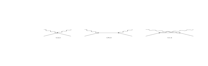
Figure 1: Feynman diagrams contributing to low energy Compton scattering.

(Note that for simplicity we take the proton to be infinitely heavy so it need not be considered.) Here the leading component is the familiar $\omega$-independent Thomson amplitude and would appear naively to lead to an energy-independent cross-section. However, this is not the case. Indeed, provided that the energy of the photon is smaller than a typical excitation energy (as is the case for optical photons), it can be shown by expanding in powers of $\omega/\Delta E$, that the cross section can be written as^?,^?

$$\quad{d\sigma\over d\Omega} = \lambda^{2}\omega^{4}|\hat{\epsilon}_{f}^{*}\cdot\hat{\epsilon}_{i}|^{2}\left(1+{\cal O}\left({\omega^{2}\over(\Delta E)^{2}}\right)\right)$$ (6)

where

$$\lambda=\alpha_{em}\sum_{n}{2|z_{n0}|^{2}\over E_{n}-E_{0}}$$ (7)

is the atomic electric polarizability, $\alpha_{em}=e^{2}/4\pi$ is the fine structure constant, and $\Delta E\sim m\alpha_{em}^{2}$ is a typical hydrogen excitation energy. We note that $\lambda\sim a_{0}^{2}\times{\alpha_{em}\over\Delta E}\sim a_{0}^{3}$ is of order the atomic volume, as will be exploited below and that the cross section itself has the characteristic $\omega^{4}$ dependence which leads to the blueness of the sky—blue light scatters much more strongly than red.^?

Now while the above derivation is rigorous and correct, it requires somewhat detailed and lengthy quantum mechanical manipulations, which obscure the relatively simple physics involved. One can avoid these problems by the use of effective field theory methods outlined above. The key point is that of scale. Since the incident photons have wavelengths $\lambda\sim 5000$A much larger than the $\sim$ 1A atomic size, then at leading order the photon is insensitive to the presence of the atom, since the latter is electrically neutral—the effective leading order Hamiltonian is simply that for the hydrogen atom

$$H_{eff}^{(0)}={\vec{p}^{2}\over 2m}+e\phi$$ (8)

and there is no interaction with the field. In higher orders, there can exist such atom-field interactions and, in order to construct the effective interaction, we demand that the Hamiltonian satisfy fundamental symmetry requirements. In particular $H_{eff}$ must be gauge invariant, must be a scalar under rotations, and must be even under both parity and time reversal transformations. Also, since we are dealing with Compton scattering, $H_{eff}$ must be quadratic in the vector potential. Actually, from the requirement of gauge invariance it is clear that the effective interaction should involve only the electric and magnetic fields

$$\vec{E}=-\vec{\nabla}\phi-{\partial\over\partial t}\vec{A},\qquad\vec{B}=\vec{\nabla}\times\vec{A}$$ (9)

since these are invariant under a gauge transformation

$$\phi\rightarrow\phi+{\partial\over\partial t}\Lambda,\qquad\vec{A}\rightarrow\vec{A}-\vec{\nabla}\Lambda$$ (10)

while the vector and/or scalar potentials themselves are not. The lowest order interaction then can involve only the rotational invariants $\vec{E}^{2},\vec{B}^{2}$ and $\vec{E}\cdot\vec{B}$. However, under spatial inversion—$\vec{r}\rightarrow-\vec{r}$—electric and magnetic fields behave oppositely—$\vec{E}\rightarrow-\vec{E}$ while $\vec{B}\rightarrow\vec{B}$—so that parity invariance rules out any dependence on $\vec{E}\cdot\vec{B}$. Likewise under time reversal—$t\rightarrow-t$ we have $\vec{E}\rightarrow\vec{E}$ but $\vec{B}\rightarrow-\vec{B}$ so such a term is also ruled out by time reversal invariance. The simplest such effective Hamiltonian must then have the form

$$H_{eff}^{(1)}=-{1\over 2}c_{E}\vec{E}^{2}-{1\over 2}c_{B}\vec{B}^{2}$$ (11)

(Forms involving time or spatial derivatives are much smaller.) We know from electrodynamics that ${1\over 2}(\vec{E}^{2}+\vec{B}^{2})$ represents the field energy per unit volume so, by dimensional arguments, in order to represent an energy in Eq. 11, $c_{E},c_{B}$ must have dimensions of volume. Also, since the photon has such a long wavelength, there is no penetration of the atom, so only classical scattering is allowed. The relevant scale must then be atomic size so that we can write

$$c_{E}=k_{E}a_{0}^{3},\qquad c_{B}=k_{B}a_{0}^{3}$$ (12)

where we expect $k_{E},k_{B}\sim{\cal O}(1)$. Finally, since for photons with polarization $\hat{\epsilon}$ and four-momentum $q_{\mu}$ we identify $\vec{A}(x)=\hat{\epsilon}\exp(-iq\cdot x)$ then from Eq. 9, $|\vec{E}|\sim\omega$, $|\vec{B}|\sim|\vec{k}|=\omega$ and

$${d\sigma\over d\Omega}\propto|<f|H_{eff}|i>|^{2}\sim\omega^{4}a_{0}^{6}$$ (13)

as found in the previous section via detailed calculation.

2.2 QCD

Now let’s return to the relevance of effective field theory to QCD. In many ways QCD represents the antithesis of QED, which can reliably be evaluated via ordinary perturbative methods to any given order in the coupling constant. As mentioned previously, one of the problems with applications of QCD at low energy is that it is written in terms of quark-gluon degrees of freedom rather than in terms of hadrons, with which experiments are done. In addition, because of asymptotic freedom, the effective quark-gluon coupling constant is large at low energies, meaning that traditional perturbative methods for solving the theory will not work. Finally, since gluons interact with each other via these large coupling, the theory is hopelessly nonlinear and one does not then have an exact solution from which an effective interaction can be derived in the low energy limit. The resolution of these problems is to construct an effective theory in terms of hadronic degrees of freedom which in the low energy regime matches onto the predictions of QCD, just as the effective interaction for Rayleigh scattering gave a fully satisfactory description of photon-atom scattering in the limit of small photon energy. In the optical scattering case we were able to deduce the form of the effective Lagrangian by requiring that it satisfy certain general principles. The same will be true for QCD—we demand that the low energy effective Lagrangian, written in terms of meson ($\phi$) and baryon ($\psi$) degrees of freedom—${\cal L}(\phi,\psi)$—have the same symmetries as does ${\cal L}_{QCD}(q,\bar{q},A_{\mu}^{i})$, in particular (broken) chiral symmetry.

3 Chiral Symmetry and Effective Lagrangians

The importance of symmetry in physics arises from Noether’s theorem which states that for every symmetry of the Hamiltonian there exists a corresponding conservation law and, associated with each such invariance, there is in general a related current $j_{\mu}$ which is conserved—i.e. $\partial^{\mu}j_{\mu}=0$. This guarantees that the associated charge will be time-independent, since

$${dQ\over dt}=\int d^{3}x{\partial j_{0}\over\partial t}=-\int d^{3}x\vec{\nabla}\cdot\vec{j}=\int_{\rm surf}d\vec{S}\cdot\vec{j}=0$$ (14)

where we have used Gauss’ theorem and the assumption that any fields are local.

Since in quantum mechanics the time development of an operator $\hat{Q}$ is given by

$${d\hat{Q}\over dt}=i[\hat{H},\hat{Q}]$$ (15)

we see that such a conserved charge must commute with the Hamiltonian. Now it is usually the case that the symmetry is realized in a Wigner-Weyl fashion wherein the vacuum (or lowest energy state) of the theory, which satisfies $\hat{H}|0>=E_{0}|0>$, is unique and has the property $\hat{Q}|0>=|0>$ since $\hat{H}(\hat{Q}|0>)=\hat{Q}(\hat{H}|0>)=E_{0}\hat{Q}|0>$. However, there exist in general a set of degenerate excited states which mix with each other under application of the symmetry charge. A familiar example of a Wigner-Weyl symmetry is isospin or SU(2) invariance. Because this is a (approximate) symmetry of the Hamiltonian, particles appear in multiplets such as $p,n$ or $\pi^{+}\pi^{0}\pi^{-}$ having identical spin-parity and (almost) the same mass and transform into one another under application of the isospin charges $\vec{I}$. However, this is not the only situation which occurs in nature. It is also possible (and in fact often the case) that the ground state of a system does not possess the same symmetry as does the Hamiltonian, in which case we say that the symmetry is realized in a Nambu-Goldstone fashion and is spontaneously broken. This phenomenon can even arise in classical mechanics. A familiar example involves a flexible rod under compression. Once the compressive force exceeds a critical value, the rod will flex, clearly breaking the axial symmetry which characterizes it. (Interestingly this particular problem was first studied by Euler in the context of beam bending!) Its connection with QCD is studied in the next section.

3.1 Spontaneous Symmetry Breaking

Chiral Symmetry

In order to understand the relevance of spontaneous symmetry breaking to QCD, we introduce the idea of ”chirality,” defined by the operators

$$\Gamma_{L,R}={1\over 2}(1\pm\gamma_{5})={1\over 2}\left(\begin{array}[]{c c }1&\mp 1\\ \mp 1&1\end{array}\right)$$ (16)

which project left- and right-handed components of the Dirac wavefunction via

$$\psi_{L}=\Gamma_{L}\psi\qquad\psi_{R}=\Gamma_{R}\psi\quad\mbox{with}\quad\psi=\psi_{L}+\psi_{R}$$ (17)

In terms of chirality states the quark component of the QCD Lagrangian can be written as

$$\bar{q}(i\not\!\!D-m)q=\bar{q}_{L}i\not\!\!Dq_{L}+\bar{q}_{R}i\not\!\!Dq_{R}-\bar{q}_{L}mq_{R}-\bar{q}_{R}mq_{L}$$ (18)

We observe then that in the limit as $m\rightarrow 0$

$${\cal L}_{\rm QCD}\stackrel{{\scriptstyle m\rightarrow 0}}{{\longrightarrow}}\bar{q}_{L}i\not\!\!Dq_{L}+\bar{q}_{R}i\not\!\!Dq_{R}-{1\over 2}{\rm tr}G_{\mu\nu}G^{\mu\nu}$$ (19)

i.e., the QCD Lagrangian is invariant under independent global left- and right-handed rotations of the light (u,d,s) quarks

$$q_{L}\rightarrow\exp(i\sum_{j}\lambda_{j}\alpha_{j})q_{L},\qquad q_{R}\rightarrow\exp(i\sum_{j}\lambda_{j}\beta_{j})q_{R}$$ (20)

This symmetry is called $SU(3)_{L}\bigotimes SU(3)_{R}$ or chiral $SU(3)\times SU(3)$. Continuing to neglect the light quark masses, we see that in a chiral symmetric world one would expect to have have sixteen—eight left-handed and eight right-handed—conserved Noether currents

$$\bar{q}_{L}\gamma_{\mu}{1\over 2}\lambda_{i}q_{L}\,,\qquad\bar{q}_{R}\gamma_{\mu}{1\over 2}\lambda_{i}q_{R}$$ (21)

Equivalently, by taking the sum and difference, we would have eight conserved vector and eight conserved axial-vector currents

$$V^{i}_{\mu}=\bar{q}\gamma_{\mu}{1\over 2}\lambda_{i}q,\qquad A^{i}_{\mu}=\bar{q}\gamma_{\mu}\gamma_{5}{1\over 2}\lambda_{i}q$$ (22)

In the vector case, this is just a simple generalization of isospin (SU(2)) invariance to the case of SU(3). There are eight ($3^{2}-1$) time-independent charges

$$F_{i}=\int d^{3}xV^{i}_{0}(\vec{x},t)$$ (23)

and there exist various supermultiplets of particles having identical spin-parity and (approximately) the same mass in configurations—singlet, octet, decuplet, etc. demanded by SU(3)invariance.

If chiral symmetry were realized in the conventional (Wigner-Weyl) fashion one would expect then there should also exist corresponding nearly degenerate but opposite parity single particle states generated by the action of the time-independent axial charges $F^{5}_{i}=\int d^{3}xA^{i}_{0}(\vec{x},t)$. Indeed since

$$H|P\rangle = E_{P}|P\rangle$$

$$H(Q_{5}|P\rangle) = Q_{5}(H|P\rangle)=E_{P}(Q_{5}|P\rangle)$$ (24)

we see that $Q_{5}|P\rangle$ must also be an eigenstate of the Hamiltonian with the same eigenvalue as $|P>$, which would seem to require the existence of parity doublets. However, experimentally this does not appear to be the case. Indeed although the $J^{p}={1\over 2}^{+}$ nucleon has a mass of about 1 GeV, the nearest ${1\over 2}^{-}$ resonce lies nearly 600 MeV higher in energy. Likewise in the case of the $0^{-}$ pion which has a mass of about 140 MeV, the nearest corresponding $0^{+}$ state (if it exists at all) is considerably higher in energy.

3.2 Goldstone’s Theorem

One can resolve this apparent paradox by postulating that parity-doubling is avoided because the axial symmetry is realized in a Nambu-Goldstone fashion and is spontaneously broken. Then according to a theorem due to Goldstone, when a (continuous) symmetry is broken in this fashion there must also be generated a massless boson having the quantum numbers of the broken generator—in this case a pseudoscalar—and when the axial charge acts on a single particle eigenstate one does not get a single particle eigenstate of opposite parity in return.^? Rather one generates one or more of these massless pseudoscalar particles

$$Q_{5}|P\rangle\sim|Pa\rangle+\cdots$$ (25)

and the interactions of such ”Goldstone bosons” with each other and with other particles is required to vanish as the four-momentum goes to zero.

Now back to QCD: According to Goldstone’s argument, one would expect there to exist eight massless pseudoscalar states—one for each spontaneously broken SU(3) axial generator, which would be the Goldstone bosons of QCD. Examination of the particle data tables reveals, however, that no such massless $0^{-}$ particles exist. There do exist eight $0^{-}$ particles—$\pi^{\pm},\pi^{0},K^{\pm},K^{0},\bar{K}^{0}\eta$ which are much lighter than their hadronic siblings. However, these states are certainly not massless and this causes us to ask what has gone wrong with what appears to be rigorous reasoning. The answer is found in the feature that our discussion thus far has neglected the piece of the QCD Lagrangian associated with quark, which can be written in the form

$${\cal L}_{\mbox{QCD}}^{m}=-(\bar{q}_{L}mq_{R}+\bar{q}_{R}mq_{L})$$ (26)

Since clearly this term breaks chiral symmetry—

$$\bar{q}_{L}mq_{R} \rightarrow \bar{q}_{L}\exp(-i\sum_{j}\lambda_{j}\alpha_{j})m\exp(i\sum_{j}\lambda_{j}\beta_{j})q_{R}$$ (27)

$$\neq \bar{q}_{L}mq_{R}$$

—we have a violation of the conditions under which Goldstone’s theorem applies. The associated pseudoscalar bosons are not required to be massless

$$m^{2}_{G}\neq 0$$ (28)

but since their mass arises only from the breaking of the symmetry the various ”would-be” Goldstone masses are expected to be proportional to the symmetry breaking parameters

$$m^{2}_{G}\propto m_{u},m_{d},m_{s}$$

To the extent that such quark masses are small the eight pseudoscalar masses are not required to be massless, merely much lighter than other hadronic masses in the spectrum, as found in nature.

3.3 Effective Chiral Lagrangian

The existence of a set of particles—the pseudoscalar mesons—which are notably less massive than other hadrons suggests the possibility of generating an effective field theory which correctly incorporates the chiral symmetry of the underlying QCD Lagrangian in describing the low energy interactions of these would-be Goldstone bosons. This can be formulated in a variety of ways, but the most transparent is done by including the Goldstone modes in terms of the argument of an exponential. Considering first SU(2), we define $U=\exp(i\vec{\tau}\cdot\phi/v)$ where $\vec{\phi}$ is the pion field and $v$ is a constant. Then under the chiral transformations

$$\psi_{L} \rightarrow L\psi_{L}$$

$$\psi_{R} \rightarrow R\psi_{R}$$ (29)

we have

$$U\rightarrow LUR^{\dagger},$$ (30)

and a form such as

$$\mbox{Tr}\partial^{\mu}U\partial_{\mu}U^{\dagger}\rightarrow\mbox{Tr}L\partial^{\mu}UR^{\dagger}R\partial_{\mu}U^{\dagger}L^{\dagger}=\mbox{Tr}\partial^{\mu}U\partial_{\mu}U^{\dagger}\,$$ (31)

is invariant under chiral rotations and can be used as part of the effective Lagrangian. However, this form is not one which describes realistic Goldstone interactions since, consistent with Goldstone’s theorem, such an invariant Lagrangian must also have zero pion mass, in contradiction to experiment. We must then add a term which accounts for quark masses in order to generate chiral symmetry breaking and thereby non-zero pion mass.

In this way, we infer that the lowest order effective chiral Lagrangian can be written as

$${\cal L}_{2}={v^{2}\over 4}\mbox{Tr}(\partial_{\mu}U\partial^{\mu}U^{\dagger})+{m^{2}_{\pi}\over 4}v^{2}\mbox{Tr}(U+U^{\dagger})\,.$$ (32)

where the subscript 2 indicates that we are working at two-derivative order or one power of chiral symmetry breaking—i.e. $m_{\pi}^{2}$. This Lagrangian is also unique, since if we expand to lowest order in $\vec{\phi}$

$$\mbox{Tr}\partial_{\mu}U\partial^{\mu}U^{\dagger}=\mbox{Tr}{i\over v}\vec{\tau}\cdot\partial_{\mu}\vec{\phi}\times{-i\over v}\vec{\tau}\cdot\partial^{\mu}\vec{\phi}={2\over v^{2}}\partial_{\mu}\vec{\phi}\cdot\partial^{\mu}\vec{\phi}\,,$$ (33)

we must reproduce the free pion Lagrangian

$${\cal L}_{2}={1\over 2}\partial_{\mu}\vec{\phi}\cdot\partial^{\mu}\vec{\phi}-{1\over 2}m^{2}_{\pi}\vec{\phi}\cdot\vec{\phi}+{\cal O}(\phi^{4})\,.$$ (34)

At the SU(3) level, including a generalized chiral symmetry breaking term, there is even predictive power—one has

$${v^{2}\over 4}\mbox{Tr}\partial_{\mu}U\partial^{\mu}U^{\dagger}={1\over 2}\sum_{j=1}^{8}\partial_{\mu}\phi_{j}\partial^{\mu}\phi_{j}+\cdots\\$$

and

$${v^{2}\over 4}\mbox{Tr}2B_{0}m(U+U^{\dagger})=\mbox{const.}-{1\over 2}(m_{u}+m_{d})B_{0}\sum_{j=1}^{3}\phi^{2}_{j}$$ (35)

$$- {1\over 4}(m_{u}+m_{d}+2m_{s})B_{0}\sum_{j=4}^{7}\phi^{2}_{j}-{1\over 6}(m_{u}+m_{d}+4m_{s})B_{0}\phi^{2}_{8}+\cdots$$

where $B_{0}$ is a constant and $m$ is the quark mass matrix. We can then identify the meson masses as

$$m^{2}_{\pi} = 2\hat{m}B_{0}$$

$$m_{K}^{2} = (\hat{m}+m_{s})B_{0}$$

$$m_{\eta}^{2} = {2\over 3}(\hat{m}+2m_{s})B_{0}\,,$$ (36)

where $\hat{m}={1\over 2}(m_{u}+m_{d})$ is the mean light quark mass. This system of three equations is overdetermined, and we find by simple algebra

$$3m_{\eta}^{2}+m_{\pi}^{2}-4m_{K}^{2}=0\,\,.$$ (37)

which is the Gell-Mann-Okubo mass relation and is well-satisfied experimentally.^?

Such effective interaction calculations in the meson sector have been developed to a high degree over the past fifteen or so years, including the inclusion of loop contributions, in order to preserve crossing symmetry and unitarity. When such loop corrections are included one must augment the effective lagrangian to include “four-derivative” terms with arbitrary coefficients which must be fixed from experiment. This program, called chiral perturbation theory, has been enormously successful in describing low energy interactions in the meson sector^?. However, in order to discuss hyperons, we must extend it to consider baryons.

4 Baryon Chiral Perturbation Theory

Our discussion of chiral techniques given above was limited to the study of the interactions of the pseudoscalar mesons (would-be Goldstone bosons) with leptons and with each other. In the real world, of course, interactions with baryons also take place and it becomes an important problem to develop a useful predictive scheme based on chiral invariance for such processes. Again much work has been done in this regard^?, but there remain important problems^?. Writing down the lowest order chiral Lagrangian at the SU(2) level is straightforward—

$${\cal L}_{\pi N}=\bar{N}(i\not\!\!{D}-m_{N}+{g_{A}\over 2}\hbox to0.0pt{/\hss}{u}\gamma_{5})N$$ (38)

where $g_{A}$ is the usual nucleon axial coupling in the chiral limit, the covariant derivative $D_{\mu}=\partial_{\mu}+\Gamma_{\mu}$ is given by

$$\Gamma_{\mu}={1\over 2}[u^{\dagger},\partial_{\mu}u]-{i\over 2}u^{\dagger}(V_{\mu}+A_{\mu})u-{i\over 2}u(V_{\mu}-A_{\mu})u^{\dagger},$$ (39)

and $u_{\mu}$ represents the axial structure

$$u_{\mu}=iu^{\dagger}\nabla_{\mu}Uu^{\dagger}$$ (40)

The quantities $V_{\mu},\,A_{\mu}$ represent external (non-dynamical) vector, axial-vector fields. Expanding to lowest order we find

$${\cal L}_{\pi N} = \bar{N}(i\hbox to0.0pt{/\hss}{\partial}-m_{N})N+g_{A}\bar{N}\gamma^{\mu}\gamma_{5}{1\over 2}\vec{\tau}N\cdot({i\over F_{\pi}}\partial_{\mu}\vec{\pi}+2\vec{A}_{\mu})$$ (41)

$$- {1\over 4F_{\pi}^{2}}\bar{N}\gamma^{\mu}\vec{\tau}N\cdot\vec{\pi}\times\partial_{\mu}\vec{\pi}+\ldots$$

which yields the Goldberger-Treiman relation, connecting strong and axial couplings of the nucleon system^?

$$F_{\pi}g_{\pi NN}=m_{N}g_{A}$$ (42)

Using the present best values for these quantities, we find

$$92.4\mbox{MeV}\times 13.05=1206\mbox{MeV}\quad\mbox{vs.}\quad 1189\mbox{MeV}=939\mbox{MeV}\times 1.267$$ (43)

and the agreement to better than two percent strongly confirms the validity of chiral symmetry in the nucleon sector. Actually the Goldberger–Treiman relation is only strictly true at the off-shell point $g_{\pi NN}(q^{2}=0)$ rather than at the physical value of the coupling $g_{\pi NN}(q^{2}=m_{\pi}^{2})$ and one expects $\sim 2\%$ discrepancy to exist. An interesting ”wrinkle” in this regard is the use of the so-called Dashen-Weinstein relation which uses simple SU(3) symmetry breaking to predict this discrepancy in terms of corresponding numbers in the strangeness changing sector.^?

4.1 Heavy Baryon Methods

Extension to SU(3) gives additional successful predictions—the baryon Gell-Mann-Okubo formula as well as the generalized Goldberger-Treiman relation. However, difficulties arise when one attempts to include higher order corrections to this formalism. The difference from the Goldstone case is that there now exist three dimensionful parameters—$m_{N}$, $m_{\pi}$ and $F_{\pi}$—in the problem rather than just $m_{\pi}$ and $F_{\pi}$. Thus loop effects can be of order $(m_{N}/4\pi F_{\pi})^{2}\sim 1$ and we no longer have a reliable perturbative scheme. A consistent power counting mechanism can be constructed provided that we eliminate the nucleon mass from the leading order Lagrangian. This is done by considering the nucleon to be very heavy. Then we can write its four-momentum as^?

$$p_{\mu}=Mv_{\mu}+k_{\mu}$$ (44)

where $v_{\mu}$ is the four-velocity and satisfies $v^{2}=1$, while $k_{\mu}$ is a small off-shell momentum, with $v\cdot k<<M$. One can construct eigenstates of the projection operators $P_{\pm}={1\over 2}(1\pm\hbox to0.0pt{/\hss}{v})$, which in the rest frame select upper, lower components of the Dirac wavefunction, so that^?

$$\psi=e^{-iMv\cdot x}(H_{v}+h_{v})$$ (45)

where

$$H_{v}=P_{+}\psi,\qquad h_{v}=P_{-}\psi$$ (46)

The $\pi N$ Lagrangian can then be written in terms of $H,h$ as

$${\cal L}_{\pi N}=\bar{H}_{v}{\cal A}H_{v}+\bar{h}_{v}{\cal B}H_{v}+\bar{H}_{v}\gamma_{0}{\cal B}^{\dagger}\gamma_{0}h_{v}-\bar{h}_{v}{\cal C}h_{v}$$ (47)

where the operators ${\cal A},{\cal B},{\cal C}$ have the low energy expansions

$${\cal A} = iv\cdot D+g_{A}u\cdot S+\ldots$$

$${\cal B} = i\not\!\!{D}^{\perp}-{1\over 2}g_{A}v\cdot u\gamma_{5}+\ldots$$

$${\cal C} = 2M+iv\cdot D+g_{A}u\cdot S+\ldots$$ (48)

Here $D_{\mu}^{\perp}=(g_{\mu\nu}-v_{\mu}v_{\nu})D^{\nu}$ is the transverse component of the covariant derivative and $S_{\mu}={i\over 2}\gamma_{5}\sigma_{\mu\nu}v^{\nu}$ is the Pauli-Lubanski spin vector and satisfies

$$S\cdot v=0,\quad S^{2}=-{3\over 4},\quad\{S_{\mu},S_{\nu}\}={1\over 2}(v_{\mu}v_{\nu}-g_{\mu\nu}),\quad[S_{\mu},S_{\nu}]=i\epsilon_{\mu\nu\alpha\beta}v^{\alpha}S^{\beta}$$ (49)

We observe that the two components H,h are coupled Eq. 47. However, the system may be diagonalized by use of the field transformation

$$h^{\prime}=h-{\cal C}^{-1}{\cal B}H$$ (50)

in which case the Lagrangian becomes

$${\cal L}_{\pi N}=\bar{H}_{v}({\cal A}+(\gamma_{0}{\cal B}^{\dagger}\gamma_{0}){\cal C}^{-1}{\cal B})H_{v}-\bar{h}^{\prime}_{v}{\cal C}h^{\prime}_{v}$$ (51)

The piece of the Lagrangian involving $H$ contains the mass only in the operator ${\cal C}^{-1}$ and is the effective Lagrangian that we seek. The remaining piece involving $h^{\prime}_{v}$ can be thrown away, as it does not couple to the $H_{v}$ physics. (In path integral language we simply integrate out this component yielding an uninteresting overall constant.) Of course, when loops are included a set of counterterms will be required and these are given at leading (two-derivative) order by

$${\cal A}^{(2)} = {M\over F_{\pi}^{2}}(c_{1}\mbox{Tr}\chi_{+}+c_{2}(v\cdot u)^{2}+c_{3}u\cdot u+c_{4}[S^{\mu},s^{\nu}]u_{\mu}u_{\nu}$$

$$+ c_{5}(\chi_{+}-\mbox{Tr}\chi_{+})-{i\over 4M}[S^{\mu},S^{\nu}]((1+c_{6})F^{+}_{\mu\nu}+c_{7}\mbox{Tr}f^{+}_{\mu\nu}))$$

$${\cal B}^{(2)} = {M\over F_{\pi}^{2}}((-{c_{2}\over 4}i[u^{\mu},u^{\nu}]+c_{6}f_{+}^{\mu\nu}+c_{7}Trf_{+}^{\mu\nu})\sigma_{\mu\nu}$$

$$- {c_{4}\over 2}v_{\mu}\gamma_{\nu}Tru^{\mu}u^{\nu})$$

$${\cal C}^{(2)} = -{M\over F_{\pi}^{2}}(c_{1}Tr\chi_{+}+(-{c_{2}\over 4}i[u^{\mu},u^{\nu}]+c_{6}f_{+}^{\mu\nu}+c_{7}trF_{+}^{\mu\nu})\sigma_{\mu\nu}$$ (52)

$$- {c_{3}\over 4}Tru^{\mu}u_{\nu}-({c_{4}\over 2}+Mc_{5})v_{\mu}v_{\nu}Tru^{\mu}u^{\nu})$$

where $f^{\pm}_{\mu\nu}=u^{\dagger}F^{R}_{\mu\nu}u\pm uF^{L}_{\mu\nu}u^{\dagger}$ and $\chi_{+}=umu+u^{\dagger}mu^{\dagger}$. Expanding ${\cal C}^{-1}$ and the other terms in terms of a power series in $1/M$ leads to an effective heavy nucleon Lagrangian of the form (to ${\cal O}(q^{3})$)

$${\cal L}_{\pi N} = \bar{H}_{v}\{{\cal A}^{(1)}+{\cal A}^{(2)}+{\cal A}^{(3)}+(\gamma_{0}{\cal B}^{(1)\dagger}\gamma_{0}){1\over 2M}{\cal B}^{(1)}$$ (53)

$$+ {(\gamma_{0}{\cal B}^{(1)\dagger}\gamma_{0}){\cal B}^{(2)}+(\gamma_{0}{\cal B}^{(2)\dagger}\gamma_{0}){\cal B}^{(1)}\over 2M}$$

$$- (\gamma_{0}{\cal B}^{(1)\dagger}\gamma_{0}){i(v\cdot D)+g_{A}(u\cdot S)\over(2M)^{2}}{\cal B}^{(1)}\}H_{v}+{\cal O}(q^{4})$$

A set of Feynman rules can now be written down and a consistent power counting scheme developed, as shown by Meissner and his collaborators.^?

4.2 Applications

As an example of the use of this formalism, called heavy baryon chiral perturbation theory (HB$\chi$pt) consider the nucleon-photon interaction. To lowest (one derivative) order we have from ${\cal A}^{(1)}$

$${\cal L}_{\gamma NN}^{(1)}=ie\bar{N}{1\over 2}(1+\tau_{3})\epsilon\cdot vN$$ (54)

while at two-derivative level we find

$${\cal L}_{\gamma NN}^{(2)}=\bar{N}\left\{{e\over 4M}(1+\tau_{3})\epsilon\cdot(p_{1}+p_{2})+{ie\over 2M}[S\cdot\epsilon,S\cdot k](1+\kappa_{S}+\tau_{3}(1+\kappa_{V})\right\}N$$

(55)

where we have made the identifications $c_{6}=\kappa_{V},\,\,c_{7}={1\over 2}(\kappa_{S}-\kappa_{V})$. We can now reproduce the low energy theorems for Compton scattering. Consider the case of the proton. At the two derivative level, we have the tree level prediction

$$(\gamma_{0}{\cal B}^{(1)\dagger}\gamma_{0}){1\over 2M}{\cal B}^{(1)}|_{\gamma pp}={e^{2}\over 2M}\vec{A}_{\perp}^{2}$$ (56)

which yields the familiar Thomson amplitude

$$\mbox{Amp}_{\gamma pp}=-{e^{2}\over M}\hat{\epsilon}^{\prime}\cdot\hat{\epsilon}$$ (57)

Again an entire literature on this subject exists, and we shall have to be content with only a brief introduction. It is now time to return to the hyperon sector to see how such chiral ideas can been applied.

5 Hyperon Properties

The quantum numbers of the ground state hyperons are easily described by noting that they, together with the nucleons, constitute an SU(3) octet. Alternatively, these values follow directly from the underlying three-quark structure which, together with the masses and magnetic moments, is listed in Table 1.

Hyperon	Quark Structure	Mass	Magnetic Moment
$\Lambda$	uds	1115.684(6)	-0.613(4)
$\Sigma^{+}$	uus	1189.37(7)	2.458(10)
$\Sigma^{0}$	uds	1192.55(8)
$\Sigma^{-}$	dds	1197.45(4)	-1.160(25)
$\Xi^{0}$	uss	1314.9(6)	-1.250(14)
$\Xi^{-}$	dss	1321.32(13)	-0.6507(25)
$\Omega^{-}$	sss	1672.5(7)	-2.02(5)

Table 1: Basic Hyperon Properties. Here masses are given in MeV and magnetic moment in nucleon magnetons.

One can achieve a basic understanding of these masses either by use of a constituent quark picture or via symmetry methods. In the former one employs the simple quark mass matrix together with an effective hyperfine interaction arising from gluon exchange

$${\cal H}_{hyp}={1\over 2}\sum_{i>j}C_{ij}\vec{s}_{i}\cdot\vec{s}_{j}\delta^{3}(\vec{r}_{i}-\vec{r}_{j})$$ (58)

and finds, e.g., in a simple bag model,

$$M_{N} = 3m_{n}\int d^{3}r(u^{2}-\ell^{2})-{3\over 8}C_{nn}$$

$$M_{\Lambda} = (2m_{n}+m_{s})\int d^{3}r(u^{2}-\ell^{2})-{3\over 8}C_{nn}$$

$$M_{\Sigma} = (2m_{n}+m_{s})\int d^{3}r(u^{2}-\ell^{2})+{1\over 8}C_{nn}-{1\over 2}C_{ns}$$

$$M_{\Xi} = (2m_{s}+m_{n})\int d^{3}r(u^{2}-\ell^{2})-{1\over 2}C_{ns}+{1\over 8}C_{ss}$$ (59)

where the subscripts $n,s$ refer to strange,nonstrange respectively and $u,\ell$ refer to the upper, lower components of the bag wavefunction.

Alternatively, one can use a symmetry-based approach. An effective SU(3) heavy baryon strong interaction chiral lagrangian for the hyperon system can be written in the form

$${\cal L} = {\rm tr}\bar{B}iv\cdot DB+d_{A}{\rm tr}\bar{B}S^{\mu}\{u_{\mu},B\}$$ (60)

$$+ f_{A}{\rm tr}\bar{B}S^{\mu}[u_{\mu},B]+d_{m}{\rm tr}\bar{B}\{\chi_{+},B\}$$

$$+ f_{m}{\rm tr}\bar{B}[\chi_{+},B]+b_{0}{\rm tr}\bar{B}B{\rm tr}\chi_{+}+\ldots$$

where $\chi_{+}$ represents the symmetry breaking due to the non-zero quark mass $m$ and has been defined below Eq. 52. At tree level one finds

$$M_{N} = \bar{M}_{0}+4(m_{K}^{2}-m_{\pi}^{2})f_{m}-4m_{K}^{2}d_{m}$$

$$M_{\Lambda} = \bar{M}_{0}-{4\over 3}(4m_{K}^{2}-m_{\pi}^{2})d_{m}$$

$$M_{\Sigma} = \bar{M}_{0}+-4m_{\pi}^{2}d_{m}$$

$$M_{\Xi} = \bar{M}_{0}-4(m_{K}^{2}-m_{\pi}^{2})f_{m}-4m_{K}^{2}d_{m}$$ (61)

where $\bar{M}_{0}=M_{0}-2(2m_{K}^{2}+m_{\pi}^{2})b_{0}.$

In either case we find a sum rule—the Gell-Mann-Okubo relation

$$M_{\Sigma}-M_{N}={1\over 2}(M_{\Xi}-M_{N})+{3\over 4}(M_{\Sigma}-M_{\Lambda})$$ (62)

which is well-satisfied experimentally—254 MeV vs. 248 MeV^?.

These results have been known for well over three decades. However, in contemporary treatments, as described above, it has become traditional to include higher order chiral contributions, and this is where one runs into difficulties—at one loop in HB$\chi$pt the nonanalytic corrections are exactly calculable and very sizable

$$\delta M_{N} = -0.31\,\,{\rm GeV},\quad\delta M_{\Sigma}=-0.62\,\,{\rm GeV}$$

$$\delta M_{\Lambda} = -0.66\,\,{\rm GeV},\quad\delta M_{\Xi}=-1.02\,\,{\rm GeV}$$ (63)

so that, e.g. the $\Xi$ mass receives a 100% correction! Of course, this is not a fatal flaw since such large nonanalytic corrections can be compensated by inclusion of appropriate higher order counterterms. Indeed the calculation has been extended to ${\cal O}(p^{4})$ by Borasoy and Meissner, who obtained^?

$$M_{N} = \bar{M}_{0}(1+0.34-0.35+0.24)$$

$$M_{\Sigma} = \bar{M}_{0}(1+0.81-0.70+0.44)$$

$$M_{\Lambda} = \bar{M}_{0}(1+0.69-0.77+0.54)$$

$$M_{\Xi} = \bar{M}_{0}(1+1.10-1.16+0.78)$$ (64)

where the nonleading terms refer to the contribution from ${\cal O}(p^{2})$ counterterms, nonanalytic pieces of ${\cal O}(p^{3})$, and ${\cal O}(p^{4})$ counterterms respectively. However, although the masses can be fit in such a picture, the structure of the series generates concern with respect to convergence. Also in this approach the Gell-Mann-Okubo discrepancy is predicted to be about 30 MeV—a factor of five larger than the 6 MeV found experimentally!.

One way out of this conundrum has been suggested by Donoghue and Holstein ^?, who point out that the origin of these large higher order corrections is the form of the ${\cal O}(p^{3})$ nonanalytic terms, which arise from the HB$\chi$pt integral

$$\int{d^{4}k\over(2\pi)^{4}}{k_{i}k_{j}\over(k_{0}-i\epsilon)(k^{2}-m^{2}+i\epsilon)}=-i\delta_{ij}{I(m)\over 24\pi}$$ (65)

If one uses dimensional regularization to evaluate this integral, the result is

$$I(m)_{\rm dim-reg}=m^{3}$$ (66)

which leads to the large nonanalytic corrections in Eq. 63, which must be cancelled by correspondingly large next order counterterms. The result is an expansion of the form (cf. Eq. 64)

$$Amp=A_{0}(1-1+1-1+\ldots)$$ (67)

However, physics tells us that this approach may be misleading. The point is that in the real world baryons have a finite size—$\sim$1 fm—and, while effects involving scales larger than this are no doubt correctly described by the effective chiral lagrangian, processes associated with smaller scales will be significantly modified by baryon structure. On the other hand the integration in Eq. 66 treats both long and short distance effects with equal weight, and this is the origin of the convergence problem. A possible solution can be found by introducing some sort of weighting function which is unity at long distance but which is damped at short distance scales, in order to simulate baryon structure. For analytic purposes it is simplest to utilize a simple dipole regulator

$$\left({\Lambda^{2}\over\Lambda^{2}-m^{2}}\right)^{2}$$ (68)

in which case the function $I(m)$ takes the form

$$I_{\Lambda}(m)=\Lambda^{4}{2m+\Lambda\over 2(m+\Lambda)^{2}}$$ (69)

Figure 2: Shown is the function $I_{\Lambda}(m)$ (monotonically decreasing curve) vs. its dimensionally regularized counterpart (monotonically increasing curve). Obviously the influence of heavy exchanged mesons is strongly suppressed in the long distance regularized version.

Notice that in the case that the mass is small compared to the cutoff $\Lambda$

$$I_{\Lambda}(m)\stackrel{{\scriptstyle m<<\Lambda}}{{\longrightarrow}}{1\over 2}\Lambda^{3}-{1\over 2}\Lambda m^{2}+m^{3}+\ldots$$ (70)

In dimensional regularization terms involving the cutoff scale $\Lambda$ are discarded leaving only the term in $m^{3}$. However, using cutoff regularization the terms in $\Lambda$ are retained, which emphasizes long distance effects and eliminates their short-distance counterparts, as can be seen by examining the opposite limit

$$I_{\Lambda}(m)\stackrel{{\scriptstyle m>>\Lambda}}{{\longrightarrow}}{\Lambda^{4}\over m}-{3\over 2}{\Lambda^{5}\over m^{2}}+\ldots$$ (71)

We observe that the function $I_{\Lambda}(m)$ then depends upon the pseudoscalar mass via inverse powers. Consequently, the pion will be strongly emphasized over its heavier eta or kaon counterparts, which is what is expected physically. This can be seen clearly in Figure 2, which plots the integral $I_{\Lambda}(m)$ together with its dimensional regularized form.

The fit to the hyperon masses which results from such a program is shown in Table 2. Obviously the convergence of the chiral expansion is now under control and the results are only weakly dependent upon the cutoff parameter. That there exists no strong cutoff dependence results from the feature that the divergent terms in $\Lambda^{3}$ and $\Lambda$ can be absorbed into renormalized values of effective parameters in the theory via

$$M_{0}^{r} = \bar{M}_{0}-(5d_{A}^{2}+9f_{A}^{2}){\Lambda^{3}\over 48\pi F_{\pi}^{2}}$$

$$d_{m}^{r} = d_{m}-(3f_{A}^{2}-d_{A}^{2}){\Lambda\over 128\pi F_{\pi}^{2}}$$

$$f_{m}^{r} = f_{m}-5d_{A}f_{A}{\Lambda\over 192\pi F_{\pi}^{2}}$$

$$b_{0}^{r} = b_{0}-(13d_{A}^{2}+9f_{A}^{2}){\Lambda\over 576\pi F_{\pi}^{2}}$$ (72)

Since such parameters are determined phenomenologically anyway, the use of such renormalized parameters is not a problem.

	Dim.	$\Lambda=300$	$\Lambda=400$	$\Lambda=500$	$\Lambda=600$
N	-0.31	0.02	0.03	0.05	0.07
$\Sigma$	-0.62	0.03	0.05	0.08	0.12
$\Lambda$	-0.66	0.03	0.06	0.12	0.17
$\Xi$	-1.03	0.04	0.08	0.12	0.17

Table 2: Nonanalytic contributions (in GeV) to baryon masses in dimensional regularization and for various values of the cutoff parameter $\Lambda$ in MeV.

That there exists cutoff dependence at all is due to the fact that we have not included the actual short distance effects. If we had a reasonable model of such pieces the result would, of course, be independent of renormalization point. The relative independence with respect to $\Lambda$ is associated with the fact that such effects are small, as expected from physics considerations. Of course, besides cutoff independence what we have lost is the consistent chiral power counting which is one of the cornerstones of the chiral procedure—cutoff regularization mixes terms of different orders. However, one can consider the price worth paying as it provides a chirally consistent picture of the physics.

Although not strictly based on chiral arguments it is important to note a parallel program which attempts to understand the hyperon masses—the $1/N_{c}$ approach being pursued at UCSD^? and which was motivated by the observation of large cancellations in parallel chiral loops calculations involving octet baryon and decuplet intermediate states. The basis of this procedure is the feature that in the large $N_{c}$ limit a spin-flavor symmetry exists for baryons—large $N_{c}$ baryons lie in irreducible representations of the spin-flavor group and one can calculate static properties in a systematic $1/N_{c}$ expansion. More precisely one can perform a simultaneous expansion in $1/N_{c}$ and in flavor breaking and the resulting mass relations can be placed in a corresponding hierarchy, whereby the higher the order in symmetry breaking and $1/N_{c}$ the better such a relation should be satisfied. An example is shown in Table 3, which is taken from work by Jenkins and Lebed^?.

Relation	$1/N_{c}$	Flavor	Expt.
$25(\bar{N}+3\bar{\Sigma}+\Lambda+2\bar{\Xi})-4(4\bar{\Delta}+3\bar{\Sigma}^{*}+2\bar{\Xi}^{*}+\Omega)$	$N_{c}$	1	…
$5(2\bar{N}+3\bar{\Sigma}+\bar{\Lambda}+2\bar{\Xi})-4(4\bar{\Delta}+3\bar{\Sigma}^{*}+2\bar{\Xi}^{*}+\Omega)$	$1/N_{c}$	1	18.2%
$5(6\bar{N}-3\bar{\Sigma}+\Lambda-4\bar{\Xi})-2(2\bar{\Delta}+3\bar{\Xi}^{*}-\Omega)$	1	$\epsilon$	20.2%
$\bar{N}-3\bar{\Sigma}+\Lambda+\bar{\Xi}$	$1/N_{c}$	$\epsilon$	5.9%
$(-2\bar{N}-9\bar{\Sigma}+3\Lambda+8\bar{\Xi})+2(2\bar{\Delta}-\bar{\Xi}^{*}-\Omega)$	$1/N_{c}^{2}$	$\epsilon$	1.1%
$35(2\bar{N}-\bar{\Sigma}-3\Lambda+2\bar{\Xi})-4(4\bar{\Delta}-5\bar{\Sigma}^{*}-2\bar{\Xi}^{*}+3\Omega)$	$1/N_{c}$	$\epsilon^{2}$	0.4%
$7(2\bar{N}-\bar{\Sigma}-3\Lambda+2\bar{\Xi})-2(4\bar{\Delta}-5\bar{\Sigma}^{*}-2\bar{\Xi}^{*}+3\Omega)$	$1/N_{c}^{2}$	$\epsilon^{2}$	0.2%
$\bar{\Delta}-3\bar{\Sigma}^{*}+3\bar{\Xi}^{*}-\Omega$	$1/N_{c}^{2}$	$\epsilon^{3}$	0.1%

Table 3: Mass relations arising in simultaneous SU(3) and $1/N_{c}$ expansion. Here the bar indicates the average mass of the multiplet.

Since both $1/N_{c}$ and the flavor breaking parameter $\epsilon$ are expected to be of order $30\%$ the results of this procedure are impressive and deserve a good deal of attention^?.

It is possible to understand how some of these relations come about by considering a $1/N_{c}$ approach within the chiral loop expansion. In this approach one treats $g_{A}$ as being ${\cal O}(N_{c})$ and $F_{\pi}$ as being ${\cal O}(\sqrt{N_{c}})$. A baryon-meson vertex then grows as $\sqrt{N_{c}}$, which means that individual meson-baryon scattering diagrams grow as $N_{c}$ and soon violate unitarity unless there exist certain consistency conditions. General arguments of $1/N_{c}$ counting produce cancellations among the diagrams contributing to chiral mass corrections when both decuplet and octet states are included as intermediate states, allowing the overall correction to be in line with general arguments although individual diagrams are not. Details of how this comes about can be found in refs. ^?,^?,^?.

6 Magnetic Moments

A second issue which has received a good deal of study over the years is that of hyperon magnetic moments. In this case a simple SU(3) analysis represents the magnetic moments in terms of lowest order couplings $f_{\mu},d_{\mu}$ via

$${\cal L}_{em}={-if_{\mu}\over 4M_{0}}{\rm tr}\bar{B}[S^{\mu},S^{\nu}][F_{\mu\nu}^{+},B]-{id_{\mu}\over 4M_{0}}{\rm tr}\bar{B}[S^{\mu},S^{\nu}]\{F_{\mu\nu}^{+},B\}$$ (73)

Equivalently, in a simple quark model the hyperon magnetic moments can be fit in terms of the corresponding quark quantities, as given in Table 4.

particle moment	SU(3)	$\mu_{s}\neq\mu_{d}$
$\mu_{p}={4\mu_{u}-\mu_{d}\over 3}$	2.6	2.8
$\mu_{n}={4\mu_{d}-\mu_{u}\over 3}$	-1.6	-1.9
$\mu_{\Lambda}=\mu_{s}$	-0.8	-0.6
$\mu_{\Sigma^{+}}={4\mu_{u}-\mu_{s}\over 3}$	2.6	2.7
$\mu_{\Sigma\Lambda}={\mu_{u}-\mu_{d}\over\sqrt{3}}$	1.7	1.6
$\mu_{\Sigma^{-}}={4\mu_{d}-\mu_{s}\over 3}$	-0.8	-1.1
$\mu_{\Xi^{0}}={4\mu_{s}-\mu_{u}\over 3}$	-1.6	-1.4
$\mu_{\Xi^{-}}={4\mu_{s}-\mu_{d}\over 3}$	-0.8	-0.5

Table 4: Theoretical values for hyperon magnetic moments in units of nucleon magnetons obtained via a global fit. The second column gives values in the lowest order chiral (SU(3)) limit wherein $\mu_{d}=\mu_{s}$ while the third column gives values in the SU(3) broken limit wherein $\mu_{s}<\mu_{d}$ due to the heavier s-quark mass.

In either case such a lowest order fit leads to the so-called Coleman-Glashow relations^?

$$\mu_{\Sigma^{+}} = \mu_{p},\quad 2\mu_{\Lambda}=\mu_{n},\quad\mu_{\Sigma^{-}}+\mu_{n}=-\mu_{p}$$

$$\mu_{\Sigma^{-}} = \mu_{\Xi^{-}},\quad\mu_{\Xi^{0}}=\mu_{n},\quad 2\mu_{\Lambda\Sigma^{0}}=-\sqrt{3}\mu_{n}$$ (74)

as well as the isospin relation

$$\mu_{\Sigma^{0}}={1\over 2}(\mu_{\Sigma^{+}}+\mu_{\Sigma^{-}})$$ (75)

Such relations also follow from a naive (degenerate) quark model picture of hyperon structure and are in fair agreement with experiment. This agreement can be considerably improved by including the u,d- and s-quark mass difference into the analysis, however, as shown in the third column of Table 4.

As in the case of the hyperon masses, the first calculation of chiral corrections was that of the leading nonanalytic piece. This was done by Caldi and Pagels^?, who found the form

$$\delta\mu_{i}={M_{0}\over 8\pi F_{\pi}^{2}}\sum_{j}\sigma_{i}^{j}m_{j}$$ (76)

where the coefficients $\sigma_{j}^{i}$ are given in ref. ^? in terms of $f_{A},g_{A}$. Corrections are large and in general destroy agreement with experiment. It is interesting to note, though, that three relations remain

$$-\mu_{\Sigma^{+}}=-2\mu_{\Lambda}-\mu_{\Sigma^{-}} \mu_{\Xi^{0}}+\mu_{\Xi^{-}}+\mu_{n}=2\mu_{\Lambda}-\mu_{p}$$

$$\mu_{\Lambda}-\sqrt{3}\mu_{\Lambda\Sigma^{0}} = \mu_{\Xi^{0}}+\mu_{n}$$ (77)

and are reasonably well satisfied by the data. Of course, overall agreement can be restored by inclusion of counterterms and a complete one loop evaluation has been done by Meissner and Steininger^?, yielding results consistent with experiment, but also lacking predictive power—

$$\mu_{p} = 4.48(1-0.49+0.11)=2.79$$

$$\mu_{n} = -2.47(1-0.34+0.12)=-1.91$$

$$\mu_{\Sigma^{+}} = 4.48(1-0.62+0.17)=2.46$$

$$\mu_{\Sigma^{-}} = -2.01(1-0.31-0.11)=-1.16$$

$$\mu_{\Sigma^{0}} = 1.24(1-0.87+0.40)=0.65$$

$$\mu_{\Lambda} = -1.24(1-0.87+0.37)=-0.61$$

$$\mu_{\Xi^{0}} = -2.47(1-0.89+0.40)=-1.25$$

$$\mu_{\Xi^{-}} = -2.01(1-0.64-0.03)=-0.65$$

$$\mu_{\Lambda\Sigma^{0}} = 2.14(1-0.53+0.19)$$ (78)

where, as before, the three contributions represent the leading ${\cal O}(p^{2})$, nonanalytic ${\cal O}(p^{3})$, and ${\cal O}(p^{4})$ counterterm contributions respectively. As in the case of the hyperon mass analysis, the basic agreement which obtains at lowest order is restored but convergence of the chiral series remains an issue.

One solution to this problem is to use long distance regularization. In this case there exists a linearly divergent component of the integral in the limit of large $\Lambda$ which can be absorbed into renormalization of the $f_{\mu},d_{\mu}$ couplings via

$$d_{\mu}^{r} = d_{\mu}+{\bar{M}_{0}\Lambda\over 4\pi F_{\pi}^{2}}d_{A}f_{A}$$

$$f_{\mu}^{r} = f_{\mu}+{\bar{M}_{0}\Lambda\over 72\pi F_{\pi}^{2}}(5d_{A}^{2}+9f_{A}^{2})$$ (79)

and when this is done the remaining chiral corrections become much smaller and under control, as found in the analogous hyperon mass analysis.

The magnetic moments have also been examineed via $1/N_{c}$ methods^??. As in the case of the masses the leading terms in the expansion are ${\cal O}(N_{c})$. However, by analyzing the corrections via a simultaneous expansion in $m_{s}$ and $1/N_{c}$ one can identify relations which are more generally valid. These can be used in order to predict values for decuplet magnetic moments. For example, the isospin relations

$$2\mu_{\Sigma^{0}} = \mu_{\Sigma^{+}}+\mu_{\Sigma^{-}}$$

$$\mu_{\Delta^{++}}-\mu_{\Delta^{+}} = \mu_{\Delta^{0}}-\mu_{\Delta^{-}}$$

$$\mu_{\Delta^{++}}-\mu_{\Delta^{-}} = 3(\mu_{\Delta^{+}}-\mu_{\Delta^{0}})$$

$$2\mu_{\Sigma^{*0}} = \mu_{\Sigma^{*+}}+\mu_{\Sigma^{*-}}$$ (80)

are valid to all orders in $N_{c}$ and $m_{s}$, while the SU(3) identities

$$0 = \mu_{\Sigma^{++}}-\mu_{\Sigma^{+}}-\mu_{\Sigma^{-}}+\mu_{\Xi^{0}}-\mu_{\Xi^{-}}$$

$$0 = \mu_{\Sigma^{*-}}-2\mu_{\Xi^{*-}}+\mu_{\Omega^{-}}$$

$$0 = \mu_{\Delta^{0}}-2\mu_{\Sigma^{*0}}+\mu_{\Xi^{*0}}$$ (81)

are valid to all orders in $1/N_{c}$ but first order in $m_{s}$. Finally, one has results

$$\mu_{\Delta^{0}} = 0$$

$$\mu_{\Delta^{+}} = 3(\mu_{p}+\mu_{n})$$

$$\mu_{\Sigma^{*+}}-\mu_{\Sigma^{*-}} = 3(-\mu_{p}+\mu_{\Sigma^{-}}+3\mu_{\Sigma^{+}}-\mu_{\Xi^{-}}+2\mu_{\Xi^{0}})$$ (82)

which are valid to all orders in $m_{s}$ and first order in $1/N_{c}$. Details of these and other relations can be found in refs. ^?.

Besides their masses and magnetic moments one of the most important properties of the hyperons is that they are unstable and decay via the weak interaction. It is this feature of hyperon physics to which we now turn.

7 Hyperon Processes

7.1 Nonleptonic Hyperon Decay

The dominant weak decay mode of the ${1\over 2}^{+}$ hyperons is the pionic channel $B\rightarrow B^{\prime}\pi$, and the most general such decay amplitude can be written in terms of an S-wave (parity-conserving) amplitude—$A$—and P-wave (parity-violating) amplitude– $B$—via

$${\rm Amp}=\bar{u}(p^{\prime})(A+B\gamma_{5})u(p)$$ (83)

Such decays have been well-studied experimentally over the years and both decay rates and asymmetries are well known. From such measurements one can determine both decay amplitudes and the resultant values are quoted in Table 5.

Mode	$A^{exp}$	$A^{th}$	$B^{exp}$	$B^{th}$
$\Lambda^{0}\rightarrow p\pi^{-}$	3.25	3.38	22.1	23.0
$\Lambda^{0}\rightarrow n\pi^{0}$	-2.37	-2.39	-15.8	-16.0
$\Sigma^{+}\rightarrow n\pi^{+}$	0.13	0.00	42.2	4.3
$\Sigma^{+}\rightarrow p\pi^{0}$	-3.27	-3.18	26.6	10.0
$\Sigma^{-}\rightarrow n\pi^{-}$	4.27	4.50	-1.44	-10.0
$\Xi^{0}\rightarrow\Lambda^{0}\pi^{0}$	3.43	3.14	-12.3	3.3
$\Xi^{-}\rightarrow\Lambda^{0}\pi^{-}$	-4.51	-4.45	16.6	-4.7

Table 5: Decay amplitudes for Nonleptonic Hyperon Decay (in units of $10^{-7}$). The theoretical amplitudes are the values arising from a lowest order chiral fit.

On the theoretical side there remain two interesting and critical issues which have been with us since the 1960’s—the origin of the $\Delta I=1/2$ rule and the S/P-wave problem^?:

• The former is the feature that $\Delta I=3/2$ amplitudes are suppressed with respect to their $\Delta I=1/2$ counterparts by factors of the order of twenty or so. This can be seen from the separation of the decay amplitudes into $\Delta I={1\over 2}$ and $\Delta I={3\over 2}$ components—cf. Table 6.

  Mode	$(A_{3}/A_{1})^{exp}$	$(B_{3}/B_{1})^{exp}$
  $\Lambda\rightarrow N\pi$	0.014	0.006
  $\Sigma\rightarrow N\pi$	-0.017	-0.047
  $\Xi\rightarrow\Lambda\pi$	0.034	0.023

  Table 6: Experimental ratio of $\Delta I={3\over 2}$ and $\Delta I={1\over 2}$ components of the decay amplitude.

  This suppression is well-known in both hyperon as well as kaon nonleptonic decay and, despite a large body of theoretical work, there still exists no simple explanation for its validity. Indeed, the lowest order weak nonleptonic $\Delta S=1$ Hamiltonian

  $${\cal O}_{W}=\bar{d}\gamma_{\mu}(1+\gamma_{5})u\bar{u}\gamma^{\mu}(1+\gamma_{5})s$$ (85)

  can be written in terms of $\Delta I={1\over 2},{3\over 2}$ components as

  $${\cal O}_{W}={1\over 2}{\cal O}_{1}+{1\over 10}{\cal O}_{2}+{1\over 15}{\cal O}_{3}+{2\over 3}{\cal O}_{4}$$ (86)

  with

  $${\cal O}_{1} = H_{A}-H_{B}$$

  $${\cal O}_{2} = H_{A}+H_{B}+2H_{C}+2H_{D}$$

  $${\cal O}_{3} = H_{A}+H_{B}+2H_{C}-3H_{D}$$

  $${\cal O}_{4} = H_{A}+H_{B}-H_{C}$$ (87)

  and

  $$H_{A} = \bar{d}\gamma_{\mu}(1+\gamma_{5})u\bar{u}\gamma^{\mu}(1+\gamma_{5})s$$

  $$H_{B} = \bar{d}\gamma_{\mu}(1+\gamma_{5})s\bar{u}\gamma^{\mu}(1+\gamma_{5})u$$

  $$H_{C} = \bar{d}\gamma_{\mu}(1+\gamma_{5})s\bar{d}\gamma^{\mu}(1+\gamma_{5})d$$

  $$H_{D} = \bar{d}\gamma_{\mu}(1+\gamma_{5})s\bar{s}\gamma^{\mu}(1+\gamma_{5})s$$ (88)

  Here ${\cal O}_{1,2}$ are octet operators carrying $\Delta I={1\over 2}$, while ${\cal O}_{3,4}$ are members of a 27-plet and carry $\Delta I={1\over 2},{3\over 2}$ respectively. Thus the $\Delta I=1/2$ and $\Delta I=3/2$ components are comparable.

  Of course, there exist important strong interaction corrections to these results. For example, taking the gluon exchange corrections to $H_{A}$ at leading order we find

  $$H_{A} \rightarrow H_{A}-{g^{2}\over 16\pi^{2}}\ln\left({M_{W}^{2}\over\mu_{H}^{2}}\right)(3H_{B}-H_{A})$$

  $$H_{B} \rightarrow H_{B}-{g^{2}\over 16\pi^{2}}\ln\left({M_{W}^{2}\over\mu_{H}^{2}}\right)(3H_{A}-H_{B})$$ (89)

  where $\mu_{H}$ represents a typical hadronic mass scale. The operators

  $${\cal O}_{\pm}={1\over 2}({\cal O}_{A}\pm{\cal O}_{B})$$ (90)

  are form-invariant—${\cal O}_{\pm}\rightarrow c_{\pm}{\cal O}_{\pm}$—with

  $$c_{\pm}=1+d_{\pm}{g^{2}\over 16\pi^{2}}\ln\left({M_{W}^{2}\over\mu_{H}^{2}}\right),\quad{\rm with}\quad d_{+}=-2,\,d_{-}=+4$$ (91)

  Using the renormalization group these corrections can be summed to leading log, yielding

  $${c_{\pm}(\mu_{H})\over c_{\pm}(M_{W})}=1+d_{\pm}{g^{2}\over 16\pi^{2}}\ln\left({M_{W}^{2}\over\mu_{H}^{2})}\right)$$ (92)

  Similarly the remaining operators can be treated, yielding renormalization group coefficients

  $$c_{1} = 1.90$$

  $$c_{2} = 0.14$$

  $$c_{3} = 0.10$$

  $$c_{4} = 0.49$$ (93)

  Such effects can bring about a $\Delta I=1/2$ enhancement of a factor of three to four^?, so we still need to account for a factor of five to six. In the case of the baryons this factor likely arises from the validity of what is called the Pati-Woo theorem^?, which requires $<B^{\prime}|{\cal O}_{2}|B>=<B^{\prime}|{\cal O}_{3}|B>=<B^{\prime}|{\cal O}_{4}|B>=0$ for the basic three-quark, color-antisymmetric component of the wavefunction. That such simple baryon-baryon matrix elements are relevant to the problem of nonleptonic hyperon decay follows from the current algebra-PCAC constraint

  $$\lim_{q\rightarrow 0}<\pi^{a}B^{\prime}|{\cal O}_{i}|B>={-i\over F_{\pi}}<B^{\prime}|[Q_{5}^{a},{\cal O}_{i}]|B>={-i\over F_{\pi}}<B^{\prime}|[I^{a},{\cal O}_{i}]|B>$$ (94)

  where the replacement of the axial charge $Q_{5}^{a}$ by the vector charge (isospin) $I^{a}$ follows from the $V+A$ character of the weak current.

  For kaons the origin of the $\Delta I={1\over 2}$ enhancement is not as transparent and appears to be associated with detailed dynamical structure. However, this is still a subject under study^?. Interestingly the one piece of possible evidence for significant $\Delta I={1\over 2}$ rule violation comes from a hyperon reaction—-hypernuclear decay^?, as will be discussed below^?.

• The S/P-wave problem is not as well known but has been a longstanding difficulty to those of us theorists who try to calculate these things. The standard approach to such decays goes back to current algebra days and expresses the S-wave (parity-violating) amplitude—$A$—as a contact term—the baryon-baryon matrix element of the axial-charge-weak Hamiltonian commutator. The corresponding P-wave (parity-conserving) amplitude—$B$—uses a simple pole model (cf. Figure 3) with the the weak baryon to baryon matrix element given by a fit to the S-wave sector. Parity-violating $BB^{\prime}$ matrix elements are neglected in accord with the Lee-Swift theorem^?, which requires the vanishing of such terms in the limit of SU(3) symmetry.

  

  Figure 3: Pole diagrams used to calculated parity-conserving nonleptonic hyperon decay.

  With this procedure one can obtain a very good S-wave fit but finds P-wave amplitudes which are in very poor agreement with experiment. An example of such a fit is shown in Table 5. (On the other hand, one can fit the P-waves, in which case the S-wave predictions are very unsatisfactory^?). Recently Skyrme as well as QCD sum rule methods have also been applied to this problem with equal lack of success^?,^?.

  The original calculations had used simple relativistic effective interactions to describe such processes. However, contemporary treatments generally involve the use of a chiral symmetry-based approach, in order to keep track of terms of given chiral order. One begins by representing the weak interaction in terms of a an effective Lagrangian given in terms of an expansion in derivatives. At lowest chiral order the form is unique

  $${\cal L}_{W}^{pv} = D{\rm tr}\left(\bar{B}\left\{u^{\dagger}\lambda_{6}u,B\right\}\right)\ +F{\rm tr}\left(\bar{B}\left[u^{\dagger}\lambda_{6}u,B\right]\right)$$

  $${\cal L}_{W}^{pc} = D_{5}{\rm tr}\left(\bar{B}\gamma_{5}\left\{u^{\dagger}\lambda_{6}u,B\right\}\right)+F_{5}\left(\bar{B}\gamma_{5}\left[u^{\dagger}\lambda_{6}u,B\right]\right)$$ (95)

  However, under a CP transformation

  $$B\rightarrow\left(i\gamma_{2}\bar{B}\right)^{T},\qquad u\rightarrow\left(u^{\dagger}\right)^{T}$$ (96)

  and it is seen that ${\cal L}_{W}^{pv}\rightarrow{\cal L}_{W}^{pv}$ but ${\cal L}_{W}^{pc}\rightarrow-{\cal L}_{W}^{pc}$ so we require $D_{5}=F_{5}=0$, which is the Lee-Swift result^?. At leading chiral order then the s-wave amplitude $A$ receives contributions directly from ${\cal L}_{W}^{pv}$ and is ${\cal O}(p^{0})$. Likewise, the p-wave amplitude $B$, which must arise from pole diagrams (Figure 3), is also apparently ${\cal O}(p^{0})$ by power counting. However, since the kinematic structure $\bar{u}\gamma_{5}u\sim\vec{\sigma}\cdot\vec{q}$ the actual behavior is $B\sim 1/\Delta m$ which is ${\cal O}(p^{-1})$.

  The S-wave amplitudes are then given in terms of just two parameters—$F,D$—via

  $$A(\Lambda\rightarrow n\pi^{0}) = {i\over 2F_{\pi}}(3F+D)$$

  $$A(\Sigma^{+}\rightarrow p\pi^{0}) = {i\sqrt{6}\over 2F_{\pi}}(D-F)$$

  $$A(\Sigma^{+}\rightarrow n\pi^{+}) = 0$$

  $$A(\Xi^{0}\rightarrow\Lambda^{0}\pi^{0}) = {i\over 2F_{\pi}}(3F-D)$$ (97)

  and a very good fit is provided by the choice

  $${F\over 2F_{\pi}}=0.92\times 10^{-7},\qquad{D\over F_{\pi}}=-0.42$$ (98)

  as can be observed in Table 5. (Note that this is one parameter less than required by SU(3) symmetry alone.) However, it is clear that the P-wave predictions are very poor with this choice.

  The first paper to examine chiral corrections to such predictions was that of Bijnens et al. who calculated the leading nonanalytic behavior, i.e. leading log corrections, to nonleptonic hyperon decay within a relativistic framework^?. However, when this was done the S-predictions no longer agreed with the data and the P-wave corrections were even larger. Subsequently, Jenkins reexamined this system within the heavy baryon formalism. As in ref. ^?, the calculation was performed at leading log order, and she found that inclusion of decuplet degrees of freedom in the loops significantly reduced the size of these corrections, leading the restoration of experimental agreement in the case of the S-wave amplitudes^?. However, the P-waves still were in significant disagreement. Perhaps in retrospect it is not so surprising that the P-waves represent such a challenge, since they involve significant cancellation in the sum of two pole contributions, which tends to enhance both any SU(3) corrections and the effect of any leading log modifications. In any case it seems clear that some sort of additional contributions are required in order to achieve an understanding of these results, and an obvious tack is to perform a complete—not just leading log—evaluation of corrections at one loop order.

  Recently Borasoy and Holstein (BH) took this approach and showed that in a one loop heavy baryon chiral perturbative approach, it is certainly possible to fit the data by selection of appropriate values of the various counterterms which arise^?. However, there are many more counterterms than data and one needs some guidance as to how to proceed. In the BH calculation, resonance saturation was used in order to decide which counterterms to utilize, but not to determine their value. Although a reasonable fit was achieved, the physics of such a result is obscure. In fact twenty years ago a possible solution to the S-/P-wave problem was proposed by Le Youaunc et al.^?, who suggested the use of SU(6) symmetry and the inclusion of contributions from the $(70,1^{-})$ intermediate states. In this case, since the parity of such resonant states is negative, such terms contribute to the parity-violating amplitude $A$ via pole diagrams, yielding

  $$\delta A(\Lambda^{0}\rightarrow n\pi^{0}) = i9\sqrt{3}C{M_{\Lambda}-M_{N}\over F_{\pi}}$$

  $$\delta A(\Sigma^{+}\rightarrow p\pi^{0}) = -i27\sqrt{2}C{M_{\Sigma}-M_{N}\over F_{\pi}}$$

  $$\delta A(\Sigma^{+}\rightarrow n\pi^{+}) = 0$$

  $$\delta A(\Xi^{0}\rightarrow\Lambda\pi^{0}) = -i12\sqrt{2}C{M_{\Xi}-M_{\Lambda}\over F_{\pi}}$$ (99)

  where $C$ is a phenomenological coupling associated with these resonance states, and we note that such contributions vanish in the limit of SU(3) symmetry, as required by the Lee-Swift theorem. Although at first sight this approach might seem to complicate matters by including an additional parameter, this is actually a very welcome modification, since our previous analysis was in contradiction to a simple constituent quark model calculation of the baryon-baryon matrix elements which yields

  $$F=-D={\sqrt{3}\over 2}G_{F}\sin\theta_{c}\cos\theta_{c}|\psi_{0}(0)|^{2}$$ (100)

  The wavefunction at the origin depends on the model (e.g. in the MIT bag picture we find $|\psi_{0}(0)|^{2}=1.15\times 10^{-2}$ GeV³) but the $D/F$ ratio is model-independent and is quite inconsistent with the value $-0.42$ found in Eq. 98. Using $C$ and $D=-0.85F$ as independent parameters, we find the very satisfactory fit shown in Table 7. The numerical value—${F\over 2F_{\pi}}\simeq 10^{-7}$—is also in the right ballpark. A full fit to s-waves and p-waves is also successful, as shown in the same table.

  Having observed the success of this resonant state insertion within the simple constituent quark model, it is natural to attempt a parallel approach from a chiral symmetry viewpoint. Although a full one loop calculation has yet to be undertaken BH, in a preliminary calculation, examined nonleptonic hyperon decay via inclusion of the lowest ${1\over 2}^{-}$ and ${1\over 2}^{+}$ resonant contributions^?. (Note that they did not include the entire complement of (70,$1^{-}$) states, which would also include the decuplet states.) A satisfactory picture of the nonleptonic decays was achieved in this approach, which reinforces the assertions of the Orsay group. However, a full one loop calculation is still needed in order to firm up this conclusion, and an important step in this direction was recently taken by Borasoy and Müller, who have evaluated the divergent components of the counterterms^?.

Mode	$A^{exp}$	$A^{th1}$	$A^{th2}$	$B^{exp}$	$B^{th1}$	$B^{th2}$
$\Lambda^{0}\rightarrow p\pi^{-}$	3.25	2.0	2.17	22.1	24.5	23.4
$\Sigma^{+}\rightarrow n\pi^{+}$	0.13	0	-0.04	42.2	44.0	44.4
$\Sigma^{-}\rightarrow n\pi^{-}$	4.27	4.42	5.33	-1.44	0.9	-1.61
$\Xi^{-}\rightarrow\Lambda\pi^{-}$	-4.51	-4.70	-4.14	16.6	19.2	14.7

Table 7: Calculated vs. experimental hyperon decay amplitudes in a simple SU(6) picture ($th1$) and in a chiral model with resonance contributions ($th2$). All amplitudes should be multipled by the factor $10^{-7}$.

It should perhaps be emphasized that both in the case of the $\Delta I={1\over 2}$ Rule and of the S-/P-wave problem, we do not require more and better data. The issues are already clear. What we need is more and better theory!

Where one does need data involves the possibility of testing the standard model prediction of CP violation, which predicts the presence of various asymmetries in the comparision of hyperon and antihyperon nonleptonic decays^?. The basic idea is that one can write the decay amplitudes in the form

$$A=|A|\exp i(\delta_{S}+\phi_{S}),\quad B=|B|\exp i(\delta_{P}+i\phi_{P})$$ (101)

where $\delta_{S},\delta_{P}$ are the strong S,P-wave phase shifts at the decay energy of the mode being considered and $\phi_{S},\phi_{P}$ are CP-violating phases which are expected to be of order $10^{-4}$ or so in standard model CP-violation. One can detect such phases by comparing hyperon and antihyperon decay parameters. Unfortunately nature is somewhat perverse here in that the larger the size of the expected effect, the more difficult the experiment. For example, the asymmetry in the overall decay rate, which is the easiest to measure, has the form

$$C_{\Gamma} = {\Gamma-\bar{\Gamma}\over\Gamma+\bar{\Gamma}}$$ (102)

$$\sim \left(-2(A_{1}A_{3}\sin(\delta_{S}^{1}-\delta_{S}^{3})\sin(\phi_{S}^{1}-\phi_{S}^{3})\right.$$

$$+ \left.B_{1}^{r}B_{3}^{r}\sin(\delta_{P}^{1}-\delta_{P}^{3})\sin(\phi_{P}^{1}-\phi_{P}^{3})\right)$$

$$/ |A_{1}|^{2}+|B_{1}^{r}|^{2}$$

where the subscripts, superscripts 1,3 indicate the $\Delta I={1\over 2},{3\over 2}$ component of the amplitude. We see then that there is indeed sensitivity to the CP-violating phases but that it is multiplicatively suppressed by both the strong interaction phases ($\delta\sim 0.1$) as well as by the $\Delta I={3\over 2}$ suppression $A_{3}/A_{1}\sim B_{3}/B_{1}\sim 1/20$. Thus we find $C\sim\phi/100\sim 10^{-6}$ which is much too small to expect to measure in present generation experiments.

More sanguine, but still not optimal, is a comparison of the asymmetry parameters $\alpha$, defined via

$$W(\theta)\sim 1+\alpha\vec{P}_{B}\cdot\hat{p}_{B^{\prime}}$$ (103)

In this case, one finds

$$C_{\alpha} = {\alpha+\bar{\alpha}\over\alpha-\bar{\alpha}}=-\sin(\phi_{S}^{1}-\phi_{P}^{1})\sin(\delta_{S}^{1}-\delta_{P}^{1})$$ (104)

$$\sim 0.1\phi\sim 4\times 10^{-4}$$

which is still extremely challenging.

Finally, the largest signal can be found in the combination

$$C_{\beta}={\beta+\bar{\beta}\over\beta-\bar{\beta}}=\cot(\delta_{S}^{1}-\delta_{P}^{1})\sin(\phi_{S}^{1}-\phi_{P}^{1})\sim\phi$$ (105)

Here, however, the parameter $\beta$ is defined via the general expression for the final state baryon polarization

$$<\vec{P}_{B^{\prime}}> = {1\over W(\theta)}\left((\alpha+\vec{P}_{B}\cdot\hat{p}_{B^{\prime}})\hat{p}_{B^{\prime}}\right.$$

$$+ \left.\beta\vec{P}_{B}\times\hat{p}_{B^{\prime}}+\gamma(\hat{p}_{B^{\prime}}\times(\vec{P}_{B}\times\hat{p}_{B^{\prime}}))\right)$$

(106)

and although, compared to $C_{\Gamma}$ and $C_{\alpha}$, the size of the effect is largest—$C_{\beta}\sim 10^{-3}$—this measurement seems out of the question experimentally.

Despite the small size of these effects, the connection with standard model CP violation and the possibility of finding larger effects due to new physics demands a no-holds-barred effort to measure these parameters.

7.2 Hypernuclear Decay

Above we mentioned the possibility of $\Delta I={1\over 2}$ Rule violation in hypernuclear decay. Since this represents an interesting and challenging area of hyperon physics, we present here a simple and concise introduction to some of the issues. However, chiral symmetry has not yet been applied to this realm, so our discussion will utilize conventional analysis.

A hypernucleus is a nuclear system in which one of the neutrons has been replaced by a $\Lambda$. As outlined above, the dominant weak decay mode of a free $\Lambda$ is the pionic decay $\Lambda\rightarrow N\pi$. One might anticipate then that in a hypernucleus, the decay rate is somewhat modified by the nuclear medium but that essentially the same physics is relevant. This is not the case, however. Indeed since the recoiling nucleon in the free decay has a momentum of only 100 MeV or so, while the Fermi momentum of a typical nucleus is $k_{F}\sim 270$ MeV, the pionic decay of the $\Lambda$ is strongly Pauli blocked^?. Instead, another mechanism, nonmesonic weak decay, takes place—$\Lambda+p\rightarrow n+p$ or $\Lambda+n\rightarrow n+n$. In this case the recoiling nucleons carry momentum $p\sim 400$ MeV $>>k_{F}$, so this becomes the dominant decay channel. Such hypernuclear decays have been studied in recent years and one now has a reasonable data base on various light and heavy nuclear systems, such as ${}_{\Lambda}^{5}He,\,\,{}_{\Lambda}^{11}B,\,\,{}_{\Lambda}^{12}C$, etc. In general one finds that the hypernuclear decay rate is roughly comparable to that for free $\Lambda$ decay and that the rates for neutron stimulated ($n\Lambda$) and proton-stimulated ($p\Lambda$) decay are about the same^?.

On the theoretical side there has also been a good deal of work, much of it based on a meson exchange picture of the effective interaction^?. The obvious meson of choice is the pion since it has the longest range and, in addition, the free $\Lambda$ decays via pion emission so the weak couplings are known. However, a realistic description must also include heavier (short-distance) exchanges of $K,\eta,\rho,K^{*},\omega,\ldots$ in order to be believable. This is also demanded phenomenologically. Indeed in a a pion-only exchange picture the effective weak interaction is of the form

$${\cal H}_{w}\sim g\bar{N}\vec{\tau}N\cdot\bar{N}\vec{\tau}\left(\begin{array}[]{l}0\\ 1\end{array}\right)\Lambda$$ (107)

Then $\Lambda n\rightarrow nn\sim g$ but $\Lambda p\rightarrow np\sim(-1-\sqrt{2}^{2})g=-3g$ so that p-stimulated decay would be strongly dominant over its n-stimulated counterpart, in contradistinction to experiment^?. Inclusion of heavier meson exchange (especially K-exchange) tends to help in this regard. However, no reasonable picture has been able to achieve the comparable values of p-stimulated and n-stimulated decay which are seen experimentally. On the other hand, all of these comprehensive meson-exchange analyses have, for simplicity, assumed the validity of the $\Delta I={1\over 2}$ Rule both for pion exchange, where it has been experimentally verified, as well as for heavy meson exchange, where no data exists. Some theorists have postulated the existence of possible $\Delta I={1\over 2}$ Rule violating four fermion interactions which may be relevant and it becomes an experimental issue whether such violations are present or not^?. The problem is that the data base is small and the uncertainties large so that substantial violation must be found in order to be believable.

At the present time there do exist suggestive results which may possibly indicate the presence of significant $\Delta I={3\over 2}$ effects in hypernuclear decay^?. This comes from analysis of nonmesonic hypernuclear decay in light systems—${{}_{\Lambda}^{4}H,{}_{\Lambda}^{5}He,{}_{\Lambda}^{4}He}$—wherein one can reasonably assume that the interaction involves only S-waves. The possible $\Lambda N$ transitions can then be categorized via

$$\begin{array}[]{ccc}{}^{S}L_{J}(initial)&{}^{S}L_{J}(final)&I_{f}\\ {}^{1}S_{0}&{}^{1}S_{0}&1\\ {}^{1}S_{0}&{}^{3}P_{0}&1\\ {}^{3}S_{1}&{}^{3}S_{1}&0\\ {}^{3}S_{1}&{}^{1}P_{1}&0\\ {}^{3}S_{1}&{}^{3}P_{1}&1\\ {}^{3}S_{1}&{}^{3}D_{1}&0\end{array}$$ (108)

and, in a semiclassical approach to such decays, one can write

$$\Gamma_{NM}({}_{\Lambda}^{A+1}Z)={N\bar{R}_{n}+Z\bar{R}_{p}\over A}\rho_{A}$$ (109)

where $\rho_{A}$ is the average nucleon density at the location of the $\Lambda$ particle and $\bar{R}_{n},\bar{R}_{p}$ denote the spin-averaged rate for the neutron-induced, proton-induced decay respectively. Defining^?

$$R_{n0} = R_{n}({}^{1}S_{0})+R_{n}({}^{3}P_{0})$$

$$R_{p0} = R_{p}({}^{1}S_{0})+R_{p}({}^{3}P_{0})$$

$$R_{n1} = R_{n}({}^{3}P_{1})$$

$$R_{p1} = R_{p}({}^{3}S_{1})+R_{p}({}^{1}P_{1})+R_{p}({}^{3}P_{1})+R_{p}({}^{3}D_{1})$$ (110)

we can write the light hypernuclear decay rates as

$$\Gamma_{NM}({}_{\Lambda}^{3}H) = {\rho_{3}\over 8}(3R_{n0}+R_{n1}+3R_{p0}+R_{p1})$$

$$\Gamma_{NM}({}_{\Lambda}^{4}H) = {\rho_{4}\over 6}(R_{n0}+3R_{n1}+2R_{p0})$$

$$\Gamma_{NM}({}_{\Lambda}^{4}He) = {\rho_{4}\over 6}(2R_{n0}+R_{p0}+3R_{p1})$$

$$\Gamma_{NM}({}_{\Lambda}^{5}He) = {\rho_{5}\over 8}(R_{n0}+3R_{n1}+R_{p0}+3R_{p1})$$ (111)

If the $\Delta I={1\over 2}$ Rule obtains then we have

$$R_{n}({}^{1}S_{0})=2R_{p}({}^{1}S_{0}),\,\,\,R_{n}({}^{3}P_{0})=2R_{p}(^{3}P_{0}),\,\,\,R_{n}({}^{3}P_{1})=2R_{p}({}^{3}P_{1})$$ (112)

Consequently,

$${R_{n1}\over R_{p1}}\leq{R_{n0}\over R_{p0}}=2$$ (113)

which should be compared with the experimental results^?

$${R_{n0}\over R_{p0}}=0.6^{+1.3}_{-0.6},\qquad{R_{n1}\over R_{p1}}=1.0^{+1.1}_{-1.0}$$ (114)

Obviously the statistics do not permit the drawing of a definitive conclusion at this time, but these suggestive results cry out for higher precision experiments as well as improved theory.

7.3 Nonleptonic Radiative Decay

Another longstanding thorn in the side of theorists attempting to understand weak decays of hyperons is the nonleptonic radiative mode $B\rightarrow B^{\prime}\gamma$^?. In this case one can write the most general decay amplitude as

$${\rm Amp} = {-ie\over M_{B}+M_{B^{\prime}}}\epsilon^{*\mu}q^{\nu}$$ (115)

$$\times \bar{u}(p^{\prime})\sigma_{\mu\nu}(C+D\gamma_{5})u(p)$$

where $C$ is the magnetic dipole (parity-conserving) amplitude and $D$ is its (parity-violating) electric dipole counterpart. There are then two primary quantities of interest in the analysis of such decays—the decay rate

$$\Gamma_{B\rightarrow B^{\prime}\gamma}={\alpha\over 2}\left(M_{B}-M_{B^{\prime}}\over M_{B}\right)^{3}(M_{B}+M_{B^{\prime}})(|C|^{2}+|D|^{2})$$ (116)

and the asymmetry parameter

$$A_{B\rightarrow B^{\prime}\gamma}=-{2{\rm Re}C^{*}D\over|C|^{2}+|D|^{2}}$$ (117)

where the angular distribution is given (in the cm frame) by

$${d\Gamma_{B\rightarrow B^{\prime}\gamma}\over d\Omega}={\Gamma_{B\rightarrow B^{\prime}\gamma}\over 4\pi}\left(1+A_{B\rightarrow B^{\prime}\gamma}\vec{\sigma}_{B}\cdot\hat{p}_{B^{\prime}}\right)\,.$$ (118)

Such decays have been the subject of a great deal of experimental and theoretical scrutiny for well over three decades. Present results are summarized in Table 8.

Mode	Branching Fraction ($\times 10^{-3}$)	Asymmetry
$\Sigma^{+}\rightarrow p\gamma$	$1.23\pm 0.06$	$-0.76\pm 0.08$
$\Lambda\rightarrow n\gamma$	$1.63\pm 0.14$
$\Xi^{0}\rightarrow\Lambda\gamma$	$1.06\pm 0.16$	$0.43\pm 0.44$
$\Xi^{0}\rightarrow\Sigma^{0}\gamma$	$3.56\pm 0.43$	$0.20\pm 0.32$
$\Xi^{-}\rightarrow\Sigma^{-}\gamma$	$0.128\pm 0.023$	$1.0\pm 1.3$
$\Omega^{-}\rightarrow\Xi^{-}\gamma$	$<0.46$

Table 8: Hyperon Radiative Decay Measurements

However, a basic theoretical understanding remains elusive. The fundamental difficulty is associated with what has come to be called “Hara’s Theorem”, which requires that in the SU(3) limit the parity violating decay amplitude must vanish for CP-conserving transitions between states of a common U-spin multiplet—i.e. $\Sigma^{+}\rightarrow p\gamma$ and $\Xi^{-}\rightarrow\Sigma^{-}\gamma$^?. The proof here is very much analogous to that which requires the vanishing of the axial tensor form factor in nuclear beta decay between members of a common isotopic spin multiplet^?. One performs a U-spin rotation $\exp(-i\pi U_{2})$ (i.e., in quark language interchanges $s,d$ quarks) on the matrix element

$$\int d^{4}xe^{iq\cdot x}<B^{\prime}|T(V_{\mu}^{em}(x){\cal H}_{w}(0)|B>$$ (119)

responsible for the radiative weak decays. Since both the electromagnetic current and weak Hamiltonian are invariant under such a transformation, we see that the amplitude for $B\rightarrow B^{\prime}\gamma$ and $B^{\prime}\rightarrow B\gamma$ must be identical when $B,B^{\prime}$ are members of a common U-spin multiplet (ı.e. $\Sigma^{+},p$ or $\Xi^{-},\Sigma^{-}$). On the other hand, CP invariance requires the form of the effective interaction to be

$${\cal H}_{eff}=-iF^{\mu\nu}\left[\bar{\psi}_{B^{\prime}}{\sigma_{\mu\nu}}(a+b\gamma_{5})\psi_{B}+\psi_{B}\sigma_{\mu\nu}(a-b\gamma_{5})\psi_{B^{\prime}}\right]$$ (120)

Only the parity-conserving interaction—$a$—is consistent with the U-spin stricture and consequently we require $b=0$, which is Hara’s theorem.

Of course, this theorem is only strictly true in the SU(3) limit. Nevertheless, since only $\sim 20\%$ SU(3) breaking effects are expected, one anticipates a relatively small photon asymmety parameter for such decays. In 1969 the first measurement of such a quantity—based upon 61 events—was reported, yielding the surprisingly large value^?

$$A_{\Sigma^{+}\rightarrow p\gamma}=-1.03^{+0.52}_{-0.42}$$ (121)

and since that time the measurement (now based on nearly 36,000 events) has been refined, but remains large and negative, as shown in Table 8.^? For these thirty years theorists have been struggling to explain this result.

Figure 4: Pole diagrams used to calculate radiative hyperon decay.

To leading chiral order the amplitude is given by the simple pole diagrams shown in Figure 4, with the weak baryon-baryon matrix elements being those determined in the pionic decay analysis discussed above. Such matrix elements—$<B^{\prime}|{\cal H}_{w}|B>$—are generally taken to be purely parity conserving since the Lee-Swift theorem asserts that all weak parity-violating baryon-baryon matrix elements must vanish in the SU(3) limit and it is in this fashion that Hara’s theorem is manifested in a pole model^?. The results of such an analysis are generally satisfactory (though only in an order of magnitude sense) for the branching ratio, but, since D=0, the asymmetry parameter is predicted to vanish for all radiative hyperon transitions, in contradistinction to experiment. It is possible to utilize a simple constituent quark model to estimate SU(3) breaking corrections.^? However, such calculations yield only $D/C\leq 0.05$ and certainly do not appear to be large enough to explain the experimental findings.

In a chiral approach, one finds similar problems. At lowest order in the chiral expansion we have

$$C_{n\Sigma^{0}} = {8\sqrt{2}\over 3}\left({M_{\Sigma}+M_{N}\over M_{\Sigma}-M_{N}}\right)Dd_{\mu}$$

$$C_{n\Lambda} = {8\over 3}\sqrt{2\over 3}\left({M_{\Lambda}+M_{N}\over M_{\Lambda}-M_{N}}\right)Dd_{\mu}$$

$$C_{\Sigma^{0}\Xi^{0}} = {8\sqrt{2}\over 3}\left({M_{\Xi}+M_{\Sigma}\over M_{\Xi}-M_{\Sigma}}\right)Dd_{\mu}$$

$$C_{\Lambda\Xi^{0}} = {8\over 3}\sqrt{2\over 3}\left({M_{\Xi}+M_{\Lambda}\over M_{\Xi}-M_{\Lambda}}\right)Dd_{\mu}$$

$$C_{p\Sigma^{+}} = C_{\Sigma^{-}\Xi^{-}}=0$$ (122)

where here $d_{\mu}$ is the d-coupling coefficient in a lowest order SU(3) fit to the magnetic moments, D is the weak SU(3) coupling defined in Eq. 97, and $D_{B^{\prime}B}=0$ for all such decays. We observe the vanishing of the entire decay rate for the U-spin doublet decays and of the asymmetry for the remaining modes, both predictions being in serious disagreement with experiment.

As in the case of the S-/P-wave puzzle for ordinary nonleptonic hyperon decay, what seems clearly required here is the inclusion of additional physics, and one may optimistically expect that the same mechanism which solves the S/P-wave problem may also work here. It is reassuring in this regard that the work two decades ago by the Orsay group proposing the inclusion of $(70,1^{-})$ states also seemed to solve the Hara’s theorem problem. In the case of a contemporary chiral approach, a one-loop calculation has been performed but has not led to a resolution, although somewhat higher values of the asymmetry can be accomodated^?. However, Borasoy and Holstein have, just as in their analysis of pionic hyperon decay, calculated within a chiral framework the contribution of the lowest ${1\over 2}^{-}$ and ${1\over 2}^{+}$ resonances to radiative hyperon decay^?. One finds, for example,

$$C_{p\Sigma^{+}} = {4(M_{\Sigma}+M_{N})\over 3}\left({1\over 3}\ell_{d}+\ell_{f}\right)(d^{*}-f^{*})\left({1\over M_{\Sigma}-M_{B*}}+{1\over M_{N}-M_{B*}}\right)$$

$$D_{p\Sigma^{+}} = 4\left({(M_{\Sigma}-M_{N})(M_{\Sigma}+M_{N})\over(M_{\Sigma}-M_{B*})(M_{N}-M_{B*})}\right)\left({1\over 3}r_{d}+r_{f}\right)(w_{d}-w_{f})$$ (123)

where here $\ell_{d},\ell_{f}$ and $r_{d},r_{f}$ represent SU(3) symmetric, antisymmetric electromagnetic couplings connecting the hyperons to ${1\over 2}^{-}$ and ${1\over 2}^{+}$ resonant states respectively, while $d^{*},f^{*}$ and $w_{d},w_{f}$ represent the corresponding weak couplings to such resonances. Note that in this picture, the form of the parity-violating coupling $D$ explicitly satisfies Hara’s theorem, as required, while while in addition, for U-spin siblings, the parity-conserving coupling $C$ vanishes unless coupling to resonances is included. The size of the electromagnetic couplings $\ell_{d}\,\ell_{f}$ can be taken from experiment, while the weak couplings $w_{f},w_{d},f^{*},d^{*}$ are determined from the previous fit to pionic nonleptonic hyperon decay, yielding a no-free-parameter prediction to this order.

What is found is that relatively large negative values of the asymmetry seem to arise naturally in such a picture. That is not to say that perfect agreement is obtained, but neither is this a complete calculation. In the ideal case, a complete one-loop calculation—including low lying resonaces—should be done for both ordinary and radiative hyperon decay and a fit to both should be performed. This lies in the future. However, in the absence of such a program, the present results are encouraging and suggest that we are on the right track.

Before closing this section, it should be noted, however, that the field is littered with red herrings, which have tended to confuse expert and nonexpert alike. These have appeared in the guise of supposed Hara’s theorem-violating models which claim to explain the radiative asymmetry results. An example is a calculation by Kamal and Riazuddin, who evaluated the amplitude for radiative decay in a simple quark model with W-exchange^?. In the static limit, these authors determined that there exists a parity-violating contribution to the decay

$${\cal H}_{pv}\sim\vec{\epsilon}\cdot(u^{\dagger}\vec{\sigma}s)\times(d^{\dagger}\vec{\sigma}u)$$ (124)

which is non-vanishing even in the limit of SU(3)-symmetry! However, gauge invariance is violated in this approach. Another gauge invariance violating procedure invokes vector dominance. However, as emphasized by Dmitrasinovic, such apparent violations are illusory^?—such results are calculated in a simplistic models and do not satisfy the usual field theoretic constraints of crossing symmetry, gauge invariance, etc. It is well-known in nuclear physics that when one calculates an electromagnetic matrix element in simple impulse approximation, the result generally violates gauge invariance unless many-body effects associated with meson exchange are included, which is often accomplished by the use of Siegert’s theorem. The same is true here—the quark calculation is the particle physics analog of the impulse approximation and, in such an elementary calculation, it is no surprise that fundamental symmetries such as gauge invariance (and Hara’s theorem) become violated. This is simply not a consistent field theoretic calculation and must therefore be discounted.

In order, however, to confirm the validity of this or any model what will be required is a set of measurements of both rates and asymmetries for such decays. In this regard, it should be noted that theoretically one expects all asymmetries to be negative in any realistic model^?—it would be very difficult to accomodate any large positive asymmetry. Thus the present particle data group listing^?

$$A_{\gamma}(\Xi^{0}\rightarrow\Lambda\gamma)=+0.43\pm 0.44$$ (125)

strongly suggests the need for a new measurement.

7.4 Hyperon Semileptonic Decay

A mode that theory does well in predicting (in fact some would say too well) is that of hyperon beta decay—$B\rightarrow B^{\prime}\ell\bar{\nu}_{\ell}$, where $\ell$ is either an electron or a muon. Since this is a semileptonic weak interaction, the decays are described in general by matrix elements of the weak vector, axial-vector currents

$$<B^{\prime}|V_{\mu}|B> = \bar{u}(p^{\prime})(f_{1}\gamma_{\mu}+{-if_{2}\over M_{B}+M_{B^{\prime}}}\sigma_{\mu\nu}q^{\nu}$$

$$+ {f_{3}\over M_{B}+M_{B^{\prime}}}q_{\mu})u(p)$$

$$<B^{\prime}|A_{\mu}|B> = \bar{u}(p^{\prime})(g_{1}\gamma_{\mu}+{-ig_{2}\over M_{B}+M_{B^{\prime}}}\sigma_{\mu\nu}q^{\nu}$$

$$+ {g_{3}\over M_{B}+M_{B^{\prime}}}q_{\mu})\gamma_{5}u(p)$$

(126)

Here the dominant terms are the vector, axial couplings $f_{1},g_{1}$ and the standard approach is simple Cabibbo theory, wherein one fits the $g_{1}$ in terms of SU(3) coefficients $f_{A},d_{A}$ and $f_{1}$ using CVC and simple F-type coupling, since the vector interaction is protected to first order from renormalization by the Ademollo-Gatto theorem.^? (Note that the lowest order chiral invariance predictions agree here with the traditional SU(3) symmetry approach.)

mode	vector	axial
pn	$1$	$f_{A}+d_{A}$
$\Lambda\Sigma^{-}$	0	${2\over\sqrt{6}}d_{A}$
$p\Lambda$	-$\sqrt{3\over 2}$	$-{1\over\sqrt{6}}(d_{A}+3f_{A})$
$\Lambda\Xi^{-}$	$\sqrt{3\over 2}$	$-{1\over\sqrt{6}}(d_{A}-3f_{A})$
$n\Sigma^{-}$	-1	$d_{A}-f_{A}$
$\Sigma^{0}\Xi^{-}$	$\sqrt{1\over 2}$	$\sqrt{1\over 2}(d_{A}+f_{A})$

Table 9: Lowest order vector and axial coupling constants for hyperon beta decay.

When this is done one finds in general a very satisfactory fit—$\chi^{2}/d.o.f\sim 3$—which can be made even better by inclusion of simple quark model SU(3) breaking effects—$\chi^{2}/d.o.f.\sim 1$^??. An output of such a fit is a value of the KM mixing parameter $V_{us}=0.220\pm 0.003$, which is in good agreement with the value $V_{us}=0.2196\pm 0.0023$ measured in $K_{e3}$ decay. However, differing assumptions about SU(3) breaking will lead to slightly modified numbers.

The importance of such a measurement of $V_{us}$ has to do with its use as an input to a test of the standard model via the unitarity prediction

$$|V_{ud}|^{2}+|V_{us}|^{2}+|V_{ub}|^{2}=1$$ (127)

From an analysis of B-decay one obtains $|V_{ub}|\sim 0.003$, which when squared leads to a negligible contribution to the unitarity sum. So the dominant effect comes from $V_{ud}$, which is measured via $0^{+}-0^{+}$ superallowed nuclear beta decay—

$$V_{ud}^{2}={2\pi^{3}\ln 2m_{e}^{-5}\over 2G_{F}^{2}(1+\Delta_{R}^{V})\bar{\cal F}t}$$ (128)

Here $\Delta_{R}^{V}=2.40\pm 0.08\%$ is the radiative correction and $\bar{\cal F}t=3072.3\pm 0.9$ sec. is the mean (modified) ft-value for such decays. Of course, there exist important issues in the analysis of such ft-values including the importance of isotopic spin breaking effects and of possible Z-dependence omitted from the radiative corrections, but if one takes the above-quoted number as being correct then^?

$$\begin{array}[]{c}V_{ud}=0.9740\pm 0.0005\\ {\rm and}\\ |V_{ud}|^{2}+|V_{us}|^{2}+|V_{ub}|^{2}=0.9968\pm 0.0014\end{array}$$ (129)

which indicates a possible violation of unitarity. If correct, this would suggest the existence of non-standard-model physics, but clearly additional work, both theoretical and experimental, is needed before drawing this conclusion.

A second interesting implication of the hyperon beta decay analysis has to do with the strange quark content of the nucleon. The issue here starts with the observation that the axial matrix element in neutron beta decay can be written in terms of the integrated u,d,s helicity content of the nucleon via

$$g_{A}(np)=\Delta u-\Delta d$$ (131)

while from hyperon beta decay we have the related result

$$g_{A}(np)\left(3f_{A}-d_{A}\over f_{A}+d_{A}\right)=\Delta u+\Delta d-2\Delta s$$ (132)

Thus far, there are only two equations but three unknowns, so we require an additional constraint. One possibility is to assume that $\Delta s=0$, i.e. to neglect the possibility of strangeness quark content of the nucleon. This is usually called the Ellis-Jaffe sum rule^? and, taking $g_{A}=1.267$ and the value $f_{A}/d_{A}=0.58$ from the simple hyperon decay fit, yields the prediction for the integrated spin structure function $g_{1}(x,Q^{2})$ measured in deep inelastic longitudinally polarized electron scattering

$$\Gamma_{1}^{p}(Q^{2}) = \int_{0}^{1}dxg_{1}(x,Q^{2})=$$ (133)

$$= {1\over 2}\left({4\over 9}\Delta u+{1\over 9}\Delta d+{1\over 9}\Delta s\right)(1+\delta_{QCD})$$

$$= ({\rm Ellis-Jaffe})\,\,\,0.171\pm 0.006\,\,{\rm at}\,\,Q^{2}=10\,\,{\rm GeV^{2}}$$

On the other hand the experimentally measured value

$$\Gamma_{1}(Q^{2})^{\rm exp}=0.120\pm 0.005\pm 0.006$$ (134)

is quite different and yields a nonzero value for the strange quark content $\Delta s=-0.11\pm 0.01$, which is perhaps not unreasonable. But it should be noted that a relatively small shift to the value $f_{A}/d_{A}\simeq 0.5$ could change this result to $\Delta s=0$. (As an aside it should be noted that these values for the $\Delta q$ are also used in order to calculate the fraction of nucleon spin which arises from valence quarks. Specifically, using the above inputs we have

$$\Delta u+\Delta d+\Delta s=0.25\pm 0.04.$$ (135)

i.e. most of the nucleon spin comes from its nonvalence components.)

Higher order chiral corrections to the lowest order SU(3) (chiral) predictions have also been investigated. The first such calculation was of the leading nonanalytic loop corrections by Bijnens, Sonoda, and Wise and yielded results in the form^?

$$g_{1}(ij)=\sqrt{Z_{i}Z_{j}}\left[\alpha_{ij}+{1\over 16\pi^{2}F_{\pi}^{2}}\sum_{k}\beta^{k}_{ij}m_{k}^{2}\ln{m_{k}^{2}\over\mu^{2}}\right]$$ (136)

where the leading order coefficients $\alpha_{ij}$ are given in Table 9, the axial renormalization couplings $\beta^{k}_{ij}$ can be found in ref. ^? and $Z_{i}$ are wavefunction renormalization factors whose leading nonanalytic form is

$$Z_{i}=1-{1\over 16\pi^{2}F_{\pi}^{2}}\kappa_{i}^{j}m_{j}^{2}\ln{m_{j}^{2}\over\mu^{2}}$$ (137)

When such corrections are included, however, the fit becomes much worse—$\chi^{2}$/d.o.f.=2.9. Of course, such problems can be solved by inclusion of higher order counterterms, but this program has yet to be carried out and in any case one wonders yet again about the phenomenological utility of the chiral expansion. The use of cutoff regularization can help. In this case the dipole-modifed integral includes a quadratic divergence which can be absorbed into renormalized values of the axial couplings via

$$d_{A}^{r} = d_{A}-{3\over 2}{\Lambda^{2}\over 16\pi^{2}F_{\pi}^{2}}d_{A}(3d_{A}^{2}+5f_{A}^{2}+1)$$

$$f_{A}^{r} = f_{A}-{1\over 6}{\Lambda^{2}\over 16\pi^{2}F_{\pi}^{2}}f_{A}(25d_{A}^{2}+63f_{A}^{2}+9)$$ (138)

and the cutoff-reularized integral brings the chiral corrections under reasonable control, as found in the case of the masses.

An alternative approach is that of evaluating the leading HB$\chi$pt loop corrections with a $1/N_{c}$ expansion while retaining the nonzero $N,\Delta$ mass difference which obtains experimentally^?. It is seen in such a calculation that the loop corrections to the axial currents retain a substantial cancellation which is due to the feature that the octet and decuplet baryons share a flavor-spin symmetry in the large $N_{c}$ limit. However, the significance of this feature as to data analysis has yet to be explored.

What is needed in the case of hyperon beta decay is good set of data including rates and asymmetries, both in order to produce a possibly improved value of $V_{us}$ and also to study the interesting issue of SU(3) breaking effects, which must be present, but whose effects seem somehow to be hidden. A related focus of such studies should be the examination of higher order—recoil—form factors such as weak magnetism ($f_{2}$) and the axial tensor ($g_{2}$). In the latter case, Weinberg showed that in the standard quark model $G=C\exp(i\pi I_{2})$-invariance requires $g_{2}=0$ in neutron beta decay $n\rightarrow pe^{-}\bar{\nu}_{e}$^?. (This result usually is called the stricture arising from “no second class currents” and has been verified to reasonable precision by correlation experiments in nuclear beta decay^?.) In the SU(3) limit one can use V-spin invariance to show that $g_{2}=0$ also obtains for $\Delta S=1$ hyperon beta decay, but in the real world this condition will be violated. A simple quark model calculation gives $g_{2}/g_{1}\sim-0.2$^? but other calculations, such as a recent QCD sum rule estimate^? suggest a larger number—$g_{2}/g_{1}\sim-0.5$. In any case good hyperon beta decay data—with rates and correlations—will be needed in order to extract the size of such effects since with only decay rate information there exists a strong correlation between the couplings $g_{1}$ and $g_{2}$.

Recently the simultaneous SU(3) and $1/N_{c}$ expansion methods so successful in understanding the hyperon masses have also been applied to the problem of hyperon beta decay^?. In this case, inclusion of symmetry breaking terms improves the quality of fit by reducing the value $\chi^{2}=62.3$ for 23 degrees of freedom which obtains using simple SU(3) symmetry to $\chi^{2}=39.2$ for 19 degrees of freedom. However, the analysis also makes a prediction that the SU(3) prediction $g_{1}/f_{1}=1.26$ for the axial coupling in $\Xi^{0}\rightarrow\Sigma^{+}e^{-}\bar{\nu}_{e}$ beta decay should be substantially reduced to lie in the range $g_{1}/f_{1}\simeq 1.02-1.07$. A quark model analysis by Ratcliffe predicts a smaller reduction—$g_{1}/f_{1}\simeq 1.15$^?. The KTeV collaboration has recently announced a preliminary number for this quantity which seems to support the simple SU(3) analysis^?, so clearly there is much more to be written on this subject.

7.5 Hyperon Polarizabilities

Since our final subject—hyperon polarizability—is not so familiar to many physicists, it is useful to give a bit of motivation. The idea goes back to simple classical physics. Parity and time reversal invariance, of course, forbid the existence of a permanent electric dipole moment for an elementary particle. However, consider the application of a uniform electric field to a charged system. Then the positive constituents making up the substructure will move in one direction and negative charges in the other—i.e. a charge separation will be generated leading to an induced electric dipole moment. The size of the edm will, for weak fields, be proportional to the strength of the applied field and the constant of proportionality between the applied field and the induced dipole moment is the electric polarizability $\alpha_{E}$

$$\vec{p}=4\pi\alpha_{E}\vec{E}$$ (139)

The interaction of this dipole moment with the field leads to an interaction energy

$$U=-{1\over 2}\vec{p}\cdot\vec{E}=-{1\over 2}4\pi\alpha_{E}\vec{E}^{2},$$ (140)

where the “extra” factor of $1\over 2$ compared to elementary physics result is due to the feature that the dipole moment is self-induced. Similarly in the presence of an applied magnetizing field $\vec{H}$ there will be generated an induced magnetic dipole moment

$$\vec{\mu}=4\pi\beta_{M}\vec{H}$$ (141)

with interaction energy

$$U=-{1\over 2}\vec{\mu}\cdot\vec{H}=-{1\over 2}4\pi\beta_{M}\vec{H}^{2}.$$ (142)

One difference here is that while the electric polarizability is required on physical grounds to be positive, the magnetic polarizability can have both paramagnetic (from magnetic moments of the substructure constituents) and diamagnetic (from motion of such constituents) components. For wavelengths large compared to the size of the system, the effective Hamiltonian describing the interaction of a system of charge $e$ and mass $m$ with an electromagnetic field is, of course, given by

$$H^{(0)}={(\vec{p}-e\vec{A})^{2}\over 2m}+e\phi,$$ (143)

and the Compton scattering cross section has the simple Thomson form

$${d\sigma\over d\Omega}=\left({\alpha_{em}\over m}\right)^{2}\left({\omega^{\prime}\over\omega}\right)^{2}{1\over 2}(1+\cos^{2}\theta),$$ (144)

where $\alpha_{em}$ is the fine structure constant and $\omega,\omega^{\prime}$ are the initial, final photon energies respectively. As the energy increases, however, so does the resolution and one must also take into account polarizability effects, whereby the effective Hamiltonian becomes

$$H_{\rm eff}=H^{(0)}-{1\over 2}4\pi(\alpha_{E}\vec{E}^{2}+\beta_{M}\vec{H}^{2}).$$ (145)

The Compton scattering cross section from such a system (taken, for simplicity, to be spinless) is then

$${d\sigma\over d\Omega} = \left({\alpha_{em}\over m}\right)^{2}\left({\omega^{\prime}\over\omega}\right)^{2}\left[{1\over 2}(1+\cos^{2}\theta)\right.$$ (146)

$$- \left.{m\omega\omega^{\prime}\over\alpha_{em}}\left({1\over 2}(\alpha_{E}+\beta_{M})(1+\cos\theta)^{2}\right.\right.$$

$$+ \left.\left.{1\over 2}(\alpha_{E}-\beta_{M})(1-\cos\theta)^{2}]\right)\right]$$

and it is clear from Eq. 146 that from careful measurement of the differential scattering cross section, extraction of these structure dependent polarizability terms is possible provided

• that the energy is large enough that these terms are significant compared to the leading Thomson piece and

• that the energy is not so large that higher order corrections become important.

In this fashion the measurement of electric and magnetic polarizabilities for the proton has recently been accomplished at SAL and at MAMI using photons in the energy range 50 MeV $<\omega<$ 100 MeV, yielding^?

$$\alpha_{E}^{p} = (12.1\pm 0.8\pm 0.5)\times 10^{-4}\;{\rm fm}^{3}$$

$$\beta_{M}^{p} = (2.1\mp 0.8\mp 0.5)\times 10^{-4}\;{\rm fm}^{3}.$$ (147)

(Results for the neutron extracted from $n-Pb$ scattering cross section measurements have been reported^?, but have been questioned^?. Extraction via studies using a deuterium target may be possible in the future^?.) Note that in practice one generally exploits the strictures of causality and unitarity as manifested in the validity of the forward scattering dispersion relation, which yields the Baldin sum rule^?

$$\alpha_{E}^{p,n} + \beta_{M}^{p,n}={1\over 2\pi^{2}}\int_{0}^{\infty}{d\omega\over\omega^{2}}\sigma_{\rm tot}^{p,n}$$ (150)

$$= \left\{\begin{array}[]{ll}(13.69\pm 0.14)\times 10^{-4}{\rm fm}^{3}&{\rm proton}\\ (14.40\pm 0.66)\times 10^{-4}{\rm fm}^{3}&{\rm neutron}\end{array}\right.$$

(151)

as a rather precise constraint because of the small uncertainty associated with the photoabsorption cross section $\sigma_{\rm tot}^{p}$.

As to the meaning of such results we can compare with the corresponding calculation of the electric polarizability of the hydrogen atom, which yields^?

$$\alpha_{E}^{H}={9\over 2}a_{0}^{2}\quad{\rm vs.}\quad\alpha_{E}^{p}\sim 10^{-3}<r_{p}^{2}>^{3\over 2}$$ (152)

where $a_{0}$ is the Bohr radius. Thus the polarizability of the hydrogen atom is of order the atomic volume while that of the proton is only a thousandth of its volume, indicating that the proton is much more strongly bound.

On the theoretical side, the electric and magnetic polarizability of the nucleon have been evaluated in heavy baryon chiral perturbation theory. At one loop—${\cal O}(p^{3})$—one finds that the theoretically predicted numbers follow strictly from chiral symmetry and are in spectacular agreement with the experimentally measured values^?

$$\alpha_{E}^{p}=10\beta_{M}^{p}={5\alpha g_{A}^{2}\over 96\pi F_{\pi}^{2}m_{\pi}}=12.2\times 10^{-4}\,{\rm fm}^{3}$$ (153)

The ${\cal O}(p^{4})$ terms have also been evaluated. At this order uncertainties due to unknown counterterms develop, but the basic agreement remains, within errors^?.

The relevance of this work to hyperon physics is that the polarizability of a hyperon can also be measured using Compton scattering, via the reaction $B+Z\rightarrow B+Z+\gamma$ extrapolated to the photon pole—i.e. the Primakoff effect. Of course, this is only feasible for charged hyperons—$\Sigma^{\pm},\Xi^{-}$, and the size of such polarizabilities predicted theoretically via SU(3) chiral perturbative techniques are somewhat smaller than that of the proton^?

$$\alpha_{E}^{\Sigma^{+}}\sim 9.4\times 10^{-4}\,{\rm fm}^{3},\qquad\alpha_{E}^{\Xi^{-}}\sim 2.1\times 10^{-4}\,{\rm fm}^{3}$$ (154)

but their measurement would be of great interest and would provide a new illumination of hyperon structure.

8 Summary

I conclude by noting that, although the first hyperon was discovered more then half a century ago and much work has been done since, the study of hyperons remains an interesting and challenging field. As I have tried to indicate above, many questions still exist as to their weak and electromagnetic interaction properties, and I suspect that such particles will remain choice targets for particle hunters well into the next century.

Acknowledgement

It is a pleasure to acknowledge helpful comments by E. Henley and R. Lebed as well as the hospitality of CTP and LNS at MIT and of INT and the Department of Physics at the University of Washington where this paper was written.

References

- [1] G.D. Rochester and C.C. Butler, Nature 160, 855 (1947).
- [2] See, e.g. P.G. Ratcliffe, hep-ph/9910544.
- [3] See, e.g. A. Manohar, ”Effective Field Theories,” in Schladming 1966: Perturbative and Nonperturbative Aspects of Quantum Field Theory, hep-ph/9606222; D. Kaplan, ”Effective Field Theories,” in Proc. 7th Summer School in Nuclear Physics, nucl-th/9506035,; H. Georgi, ”Effective Field Theory,” in Ann. Rev. Nucl Sci. 43, 209 (1995).
- [4] J. Gasser and H. Leutwyler, Ann. Phys. (NY) 158, 142 (1984); Nucl. Phys. B250, 465 (1985).
- [5] For a pedagogical introduction see J.F. Donoghue, E. Golowich and B.R. Holstein, Dynamics of the Standard Model, Cambridge University Press, New York (1992).
- [6] B.R. Holstein, Am. J. Phys. 67, 422 (1999).
- [7] B.R. Holstein, Topics in Advanced Quantum Mechanics, Addison-Wesley, Reading, MA (1992).
- [8] J.J. Sakurai, Advanced Quantum Mechanics, Addison-Wesley, Reading, MA (1967).
- [9] A corresponding classical physics discussion is given in R.P Feynman, R.B. Leighton, and M. Sands, The Feynman Lecures on Physics, Addison-Wesley, Reading, MA, (1963) Vol. I, Ch. 32.
- [10] J. Goldstone, Nuovo Cim. 19, 154 (1961); J. Goldstone, A. Salam and S. Weinberg, Phys. Rev. 127, 965 (1962).
- [11] M. Gell-Mann, CalTech Rept. CTSL-20 (1961); S. Okubo, Prog. Theo. Phys. 27, 949 (1962).
- [12] J. Gasser, M. Sainio, and A. Svarc, Nucl. Phys. B307, 779 (1988).
- [13] V. Bernard, N. Kaiser, and U.G. Meissner, Int. J. Mod. Phys. E4, 193 (1995).
- [14] M. Goldberger and S.B. Treiman, Phys. Rev. 110, 1478 (1958).
- [15] R. Dashen and M. Weinstein, Phys. Rev. 188, 2330 (1969); B.R. Holstein, ”Nucleon Axial Matrix Elements,” nucl-th/9806036; J.L. Goity, R. Lewis, and M. Schvelinger, ”The Goldberger-Treiman Discrepancy in SU(3),” hep-ph/9901374.
- [16] E. Jenkins and A.V. Manohar, in Effective Theories of the Standard Model, ed. U.-G. Meißner, World Scientific, Singapore (1992).
- [17] Here we follow V. Bernard, N. Kaiser, J. Kambor and Ulf-G. Meißner, Nucl. Phys. B388, 315 (1992).
- [18] B. Borasoy and U.-G. Meissner, Phys. Lett. B365, 285 (1986); Ann. Phys. (NY) 254, 192 (1997); P. Langacker and H. Pagels, Phys. Rev. D8, 4595 (1975).
- [19] J.F. Donoghue and B.R. Holstein, Phys. Lett. B436, 331 (1998); J.F. Donoghue, B.R. Holstein, and B. Borasoy, Phys. Rev. D59, 036002 (1999).
- [20] For a review see E. Jenkins, Ann. Rev. Nucl. Part. Sci. 48, 81 (1998). See also A.V. Manohar, hep-ph/9802419 and R. Lebed, Czech. J. Phys. 49, 1273 (1999).
- [21] E. Jenkins and R.F. Lebed, Phys. Rev. D52, 282 (1995).
- [22] hep-ph/0005038.
- [23] R. Dashen and A.V. Manohar, Phys. Lett. B315, 425 and 447 (1993).
- [24] E. Jenkins, Phys. Lett B315, 431, 441, and 447 (1993).
- [25] R. Dashen et al., Phys. Rev. D49, 4713 (1994).
- [26] S. Coleman and S.L. Glashow, Phys. Rev. Lett. 6, 423 (1961).
- [27] D.G. Caldi and H. Pagels, Phys. Rev. D10, 3739 (1974).
- [28] U.-G. Meissner and S. Steininger, Nucl. Phys. B499, 349 (1997).
- [29] E. Jenkins and A.V. Manohar, Phys. Lett. B335, 452 (1994).
- [30] J. Dai, R. Dashen, E. Jenkins, and A.V.. Manohar, Phys. Rev. D53, 273 (1996).
- [31] M.A. Luty, J. March-Russell, and M. White, Phys. Rev. D51, 2332 (1995).
- [32] J.D. Bjorken and S.D. Drell, Relativisitic Quantum Mechanics, McGraw-Hill, New York (1964).
- [33] F. Gilman and M. Wise, Phys. Rev. D20 (1979) 2392.
- [34] J. Pati and C.Woo, Phys. Rev. D3 (1971) 2920; K. Muira and T. Minamikawa, Prog. Theor. Phys. 38 (1967) 954; J. Körner, Nucl. Phys. B25 (1970) 282.
- [35] See, e.g. G. Buchalla, A.J. Buras, and M.E. Lautenbacher, Rev. Mod. Phys. 68 (1996) 1125; J. Bijnens, hep-ph/9907514.
- [36] See, e.g. J.F. Dubach, G.B. Feldman, B.R. Holstein, and L. de la Torre, Ann. Phys. (NY) 249 (1996) 146.
- [37] See, e.g. J.F. Dubach, G.B. Feldman, B.R. Holstein, and L. de la Torre, Ann. Phys. (NY), 249 (1996) 146.
- [38] D.G. Dumm, A.J. Garcia, and N.N. Scoccola, hep-ph/0001042.
- [39] E.M. Henley, W.Y.P. Hwang, and L.S. Kisslinger, hep-ph/9912530.
- [40] B.W. Lee and A. Swift, Phys. Rev. 136 (1964) B228.
- [41] J.F. Donoghue, E. Golowich, and B.R. Holstein, Phys. Rept. 131 (1986) 319.
- [42] J. Bijnens, H. Sonoda, and M. Wise, Nucl. Phys. B261, 185 (1985).
- [43] E. Jenkins, Nucl. Phys. B375, 561 (1992).
- [44] B. Borasoy and B.R. Holstein, Eur. Phys. J. C6, 85 (1999).
- [45] A. Le Yaouanc et al., Nucl. Phys. B149 (1979) 312.
- [46] B. Borasoy and B.R. Holstein, Phys. Rev. D59, 054025 (1999).
- [47] B. Borasoy and G. Müller, Phys. Rev. D62, 054020 (2000).
- [48] J.F. Donoghue, X.G. He, and S. Pakvasa, Phys. Rev. D34 (1986) 833; S. Pakvasa, hep-ph/9910232.
- [49] W. Cheston and H. Primakoff, Phys. Rev. 92, 1537 (1953).
- [50] J.J. Szymanski et al., Phys. Rev. C43, 849 (1991).
- [51] J.F. Dubach, G.B. Feldman, B.R. Holstein, and L. de la Torre, Ann. Phys. (NY) 249, 146 (1996); A. Parreno, A. Ramos and C. Bennhold, Phys. Rev. C56, 339 (1997).
- [52] M Shmatikov, Nucl. Phys. A580, 538 (1994).
- [53] Kk. Maltman and M. Shmatikov, Phys. Lett. B331, 1 (1994).
- [54] See, e.g. W.M. Alberico and G. Garbarino, nucl-th/0001012.
- [55] M.M. Block and R.H. Dalitz, Phys. Rev. Lett. 11, 96 (1963).
- [56] See, e.g. J. Lach and P. Zencykowski, Int. J. Mod. Phys. A10 (1995) 3817.
- [57] Y. Hara, Phys. Rev. Lett. 12 (1964) 378; R.H. Graham and S. Pakvasa, Phys. Rev. 140 (1965) B1144.
- [58] B.R. Holstein and S.B. Treiman, Phys. Rev. C3 (1971) 1921.
- [59] L. Gershwin et al., Phys. Rev. 188, 2077 (1969).
- [60] Particle Data Group, Phys. Rev. D54 (1996) 1.
- [61] See, e.g., E. Golowich and B.R. Holstein, Phys. Rev. D26 (1982) 182.
- [62] H. Neufeld, Nucl. Phys. B402, 166 (1993).
- [63] B. Borasoy and B.R. Holstein, Phys. Rev. D59 (1999) 054019.
- [64] A. Kamal and Riazuddin, Phys. Rev. D28, 2317 (1983).
- [65] V. Dmitrasinovic, Phys. Rev. D54, 5899 (1996); Phys. Rev. D60, 018902 (1999).
- [66] I am very grateful to P. Zencykowski for a discussion of this point.
- [67] M. Ademollo and R. Gatto, Phys. Rev. Lett. 13, 264 (1964).
- [68] See, e.g., J.F. Donoghue, B.R. Holstein, and S. Klimt, Phys. Rev. D35 (1987) 934; R. Flores-Mendieta, A. Garcia, and G. Sanchez-Colon, Phys. Rev. D54 (1996) 6855.
- [69] P.G. Ratcliffe, hep-ph/9710458.
- [70] J. Hardy and I. Towner, nucl-th/9807049.
- [71] J. Ellis and R.L. Jaffe, Phys. Rev. D9, 1444 (1974) and D10, 1669 (1974).
- [72] J. Bijnens, H. Sonoda and M.B. Wise, Nucl. Phys. B261, 185 (1985).
- [73] R. Flores-Mendieta, C.P Hofmann, E. Jenkins, and A. Manohar, hep-ph/0001218.
- [74] S. Weinberg, Phys. Rev. 112 (1958) 1375.
- [75] T. Minimisono et al., Phys. Rev. Lett. 80, 4132 (1998).
- [76] J.F. Donoghue and B.R. Holstein, Phys. Rev. D25 (1982) 206.
- [77] H. Shiomi, Nucl. Phys. A603, 281 (1996).
- [78] R. Flores-Mendita, E. Jenkins, and A.V. Manohar, Phys. Rev. D58, 094028 (1998).
- [79] R.P. Ratcliffe, Phys. Rev. D59, 014038 (1999).
- [80] A. Affolder et al., Phys. Rev. Lett. 82, 3751 (1999).
- [81] F.J. Federspiel et al., Phys. Rev. Lett. 67 (1991) 1511; A.L. Hallin et al., Phys. Rev. C48 (1993) 1497; A. Zieger et al., Phys. Lett. B278 (1992) 34; B.E. MacGibbon et al., Phys. Rev. C52 (1995) 2097.
- [82] J. Schmiedmayer et al., Phys. Rev. Lett. 66 (1991) 1015.
- [83] L. Koester, Phys. Rev. C51 (1995) 3363.
- [84] S. Beane, M. Malheiro, D.R. Phillips, and U. van Kolck, Nucl. Phys. A656 (1999) 367.
- [85] D. Babusci, G. Giordano, and G. Matone, Phys. Rev. C57 (1998) 291.
- [86] E. Merzbacher, Quantum Mechanics, Wiley, Nw York (1998), Ch. 18.
- [87] V. Bernard, N. Kaiser, A. Schmidt, and U.-G. Meissner, Phys. Lett B319, 269 (1993); Z. Phys. A348, 317 (1994).
- [88] V. Bernard, N. Kaiser, J. Kambor, and U.-G. Meissner, Phys. Rev. D46 (1992) 2756.