1 Introduction

Magnetic catalysis is the phenomenon of dynamical symmetry breaking induced by external magnetic or chromomagnetic fields. This kind of influence of an external magnetic field $H$ was for the first time observed in the study of the (2+1)-dimensional chiral invariant Gross–Neveu model [1]. In that case, an arbitrary weak external magnetic field lead to dynamical chiral symmetry breaking (D$\chi$SB) even for an arbitrary small coupling constant [2, 3]. This phenomenon is explained by the effective reduction of space-time dimensions in the external magnetic field and, correspondingly, by strengthening the role of the infrared divergences in the vacuum reorganization [4]. Later, it has been shown that spontaneous chiral symmetry breaking can be induced by an external chromomagnetic field as well [5, 6, 7]. Moreover, basing upon the study of a number of field theories, it has been argued that magnetic catalysis of D$\chi$SB may have a universal, i.e. model independent, character [8]. In a recent paper [9], a $P$ symmetric 3-dimensional Gross–Neveu model has been studied, and the external magnetic field proved to be a catalyst for spontaneous symmetry breaking again, this time for $P$ parity breaking. Magnetic catalysis has already found its applications in cosmology and astrophysics [10], and in constructing the theory of high-temperature superconductivity [9, 11]. It is evident that this phenomenon may be of crucial importance for various processes in the presence of an external magnetic field, where the dynamical symmetry breaking takes place, i.e. in the elementary-particle physics, condensed-matter physics, physics of neutron stars etc.

As it is well known [13], the high temperature superconductivity is observed in antiferromagnetic materials like La₂CuO₄, where conduction electrons are concentrated in planes formed by atoms of Cu and O. In recent experimental studies of this phenomenon [14], it was found out that at temperatures much lower than the temperature of transition to the superconducting state, the external magnetic field induces a parity-breaking phase transition. Thus, the problem of studying magnetic catalysis in high-temperature superconductivity becomes quite urgent. The above arguments are first of all applicable to (2+1)-dimensional field-theoretical models of high-temperature superconductivity.

In the present paper, we consider the influence of an external magnetic field on one of these 3d models with a four-fermion interaction Lagrangian of the form

$$L=\sum_{a=1}^{N}\bar{\psi}_{a}i\hat{\partial}\psi_{a}+\frac{G_{1}}{2N}(\sum_{a=1}^{N}\bar{\psi}_{a}\psi_{a})^{2}+\frac{G_{2}}{2N}(\sum_{a=1}^{N}\bar{\psi}_{a}\tau\psi_{a})^{2},$$ (1)

where $\hat{\partial}\equiv\Gamma^{\mu}\partial_{\mu}\,$, fields $\psi_{a}$ are transformed according to the fundamental representation of the $U(N)$ group introduced in order to employ the nonperturbative $1/N$-expansion method. Moreover, $\psi_{a}$ is a four-component Dirac spinor for every value of $a=1,2,...,N$ (corresponding indices are omitted). The action with the Lagrangian (1) is invariant under two discrete transformations, one of them being parity ($P$), and the other is chiral symmetry $\Gamma_{5}$ (these operations, as well as the matrix $\tau$ are defined in the Appendix, where the algebra of $\Gamma^{\mu}$ matrices for the spinor reducible 4-dimensional representation of the Lorentz group is also presented).

The model (1) at $H=0$ has already been studied in papers [15], and a corresponding gauge version of the model was considered in  [16]. This interest is mainly justified by the fact, that in a number of lattice models, describing dynamic effects in quantum antiferromagnetics in two spatial dimensions (e.g., high temperature superconductivity), going to continuum limit renders theories of the type (1).

In contrast to simplest Gross-Neveu models, there are two different structures with four-fermion interaction in the Lagrangian (1). Hence, two different fermion condensates can exist in the theory: one of them, $\langle\bar{\psi}\psi\rangle$, is the order parameter for chiral symmetry, and the other one, $\langle\bar{\psi}\tau\psi\rangle$, characterizes spontaneous breaking of parity. The condensate that provides for the lowest vacuum energy corresponds to the symmetry that is broken. The above arguments are fully applicable to the case of nonzero field $H\neq 0$. Therefore, the magnetic catalysis effects in the model (1) and in simplest Gross-Neveu models should be qualitatively different.

Our main goal is to study characteristics of the magnetic catalysis in the $P\times\Gamma_{5}$-invariant model (1). At first, we are going to find out whether spontaneous symmetry breaking of the initial symmetry is induced by an external magnetic field. If this is the case, the question is whether both $P$ and $\Gamma_{5}$ symmetries are broken simultaneously, or the vacuum of the model retains symmetry with respect to only one of the two discrete transformations. If the latter possibility is realized, then a question arises how the residual symmetry of the model depends on the values of coupling constants $G_{1,2}$, etc. We demonstrate, that under certain conditions in the framework of the field theory (1), a parity breaking phase transition induced by an external magnetic field is possible.

2 Phase structure of the model at $H=0$

Before considering the influence of the nonzero external magnetic field $H$ on the vacuum of the model (1), its phase structure will be studied at $H=0$. To this end, the auxiliary Lagrangian

$$\tilde{L}=\bar{\psi}i\hat{\partial}\psi+\sigma_{1}(\bar{\psi}\psi)+\sigma_{2}(\bar{\psi}\tau\psi)+\frac{N\sigma_{1}^{2}}{2G_{1}}+\frac{N\sigma_{2}^{2}}{2G_{2}}$$ (2)

is introduced, where $\sigma_{1,2}$ are auxiliary boson fields, and summation over indices $a$ of the auxiliary group $U(N)$ is implicitly performed here and in what follows. The field theories (1) and (2) are equivalent, since by means of the equations of motion the fields $\sigma_{1,2}$ can be excluded from (2) and the Lagrangian (1) obtained. It is easily shown that the auxiliary fields are transformed with respect to discrete symmetries $P$ and $\Gamma_{5}$ in the following way:

$$\begin{array}[]{l}P:~{}\sigma_{1}(t,x,y)\rightarrow\sigma_{1}(t,-x,y);~{}~{}\sigma_{2}(t,x,y)\rightarrow-\sigma_{2}(t,-x,y);\\ \Gamma_{5}:~{}\sigma_{1}(t,x,y)\rightarrow-\sigma_{1}(t,x,y);~{}~{}\sigma_{2}(t,x,y)\rightarrow\sigma_{2}(t,x,y),\end{array}$$ (3)

i.e. $\sigma_{1}$ is a scalar field, and $\sigma_{2}$ is pseudoscalar one. Starting from the Lagrangian (2), one can find the effective action of the theory, which has the following form in the one-loop approximation (i.e. in the leading order of the $1/N$ expansion):

$$S_{\rm eff}(\sigma_{1},\sigma_{2})=-N\int d^{3}x\left(\frac{\sigma_{1}^{2}}{2G_{1}}+\frac{\sigma_{2}^{2}}{2G_{2}}\right)-i\mbox{Sp}\ln\Delta,$$ (4)

where $\Delta=i\hat{\partial}+\sigma_{1}+\sigma_{2}\tau$. Here, the fields $\sigma_{1,2}$ are functions of space-time points. To obtain the effective potential of the model, the definition has to be used

$$\left.V_{0}(\sigma_{1},\sigma_{2})\int d^{3}x=-S_{\rm eff}(\sigma_{1},\sigma_{2})\right|_{\sigma_{1},\sigma_{2}=\mathop{\rm const}\nolimits},$$ (5)

where boson fields are assumed to be independent of coordinates. With the help of (4) and (5), the following expression for the effective potential of the model (1) can be found in the leading order of the $1/N$ expansion:

$$V_{0}(\sigma_{1},\sigma_{2})=\frac{N\sigma_{1}^{2}}{2G_{1}}+\frac{N\sigma_{2}^{2}}{2G_{2}}-N\sum_{k=1}^{2}\int\frac{d^{3}p}{(2\pi)^{3}}\ln(p^{2}+M^{2}_{k}),$$ (6)

where $M_{1,2}=|\sigma_{2}\pm\sigma_{1}|$, and integration is performed over Euclidean momentum. Integration in (6) over the domain $0\leq p^{2}\leq\Lambda^{2}$ yields:

$$V_{0}(\sigma_{1},\sigma_{2})=N\sum_{k=1}^{2}\left[\frac{\sigma_{k}^{2}}{2}\left(\frac{1}{G_{k}}-\frac{2\Lambda}{\pi^{2}}\right)+\frac{M_{k}^{3}}{6\pi}\right].$$ (7)

Now, in order to exclude the cutoff parameter $\Lambda$ from (7), we introduce the renormalized coupling constants with the help of the following normalization conditions:

$$\left.\frac{1}{N}\frac{\partial^{2}V_{0}}{(\partial\sigma_{1})^{2}}\right|_{\begin{array}[]{l}\scriptstyle{\sigma_{1}=\nu_{1}}\\[-10.0pt] \scriptstyle{\sigma_{2}=0}\end{array}}=\frac{1}{G_{1}}-\frac{2\Lambda}{\pi^{2}}+\frac{2\nu_{1}}{\pi}\equiv\frac{1}{g_{1}(\nu_{1})},$$ (10)

$$\left.\frac{1}{N}\frac{\partial^{2}V_{0}}{(\partial\sigma_{2})^{2}}\right|_{\begin{array}[]{l}\scriptstyle{\sigma_{1}=0}\\[-10.0pt] \scriptstyle{\sigma_{2}=\nu_{2}}\end{array}}=\frac{1}{G_{2}}-\frac{2\Lambda}{\pi^{2}}+\frac{2\nu_{2}}{\pi}\equiv\frac{1}{g_{2}(\nu_{2})}.$$ (13)

Relations (13) enable us to write the effective potential in terms of the ultraviolet finite quantities

$$V_{0}(\sigma_{1},\sigma_{2})=N\sum_{k=1}^{2}\left[\frac{\sigma_{k}^{2}}{2g_{k}}+\frac{M_{k}^{3}}{6\pi}\right],$$ (14)

where ($i=1,2$):

$$\frac{1}{g_{i}}=\frac{1}{g_{i}(\nu_{i})}-\frac{2\nu_{i}}{\pi}=\frac{1}{G_{i}}-\frac{1}{G_{c}}$$ (15)

and $G_{c}=\pi^{2}/(2\Lambda)$. We remind that the coupling constants $G_{i}$ ($g_{i}(\nu_{i})$) depend (do not depend) on the cutoff parameter $\Lambda$ and do not depend (depend) on the normalization masses $\nu_{i}$. By virtue of this, (15) leads us to the conclusion that the constants $g_{i}$ depend neither on $\nu_{i}$, nor on $\Lambda$, i.e. the effective potential $V_{0}$ is a renormalization invariant finite quantity (i.e., without ultraviolet divergences).

Thus, we have indeed demonstrated that the model (1) is renormalizable in the leading order of the $1/N$ expansion. The complete proof of its renormalizability is not intended in the present paper. However, we believe this to be true, relying on the results of the review paper [17], where the simplest 3-dimensional models with four-fermion interaction were proved to be renormalizable in the framework of the nonperturbative $1/N$ expansion method.

It is well known that the phase structure of any theory is to a great extent determined by the symmetry of the global minimum of its effective potential. In order to avoid cumbersome formulas, we omit intermediate calculations, related to the study of the absolute minimum of the potential $V_{0}(\sigma_{1},\sigma_{2})$ (14) and present here the final result – the phase portrait of the model (1), depicted in Fig. 1 (similar analysis of the effective potentials for a whole series of the theories with the four-fermion interaction is carried out in [6, 18], and, if required, it can be easily performed here). In this figure, the plane $(g_{1},g_{2})$ of coupling constants (15) is divided into five regions, in each of which one of the possible phases of the model is realized: A, B, C. In the phase A, where $g_{1,2}>0$, corresponding to small values of the coupling constants $G_{1,2}<G_{c}$, the global minimum of the function $V_{0}(\sigma_{1},\sigma_{2})$ is at the origin $(\sigma_{1}=\sigma_{2}=0)$, and hence, the ground state of the system in this phase is $P$ and $\Gamma_{5}$ symmetric. In phases B and C, where at least one of the coupling constants $G_{i}$ is greater than $G_{c}$, the point of the potential global minimum is correspondingly at $\sigma_{1}=0,\;\sigma_{2}=-\pi/g_{2}$ and $\sigma_{1}=-\pi/g_{1},\;\sigma_{2}=0$. Hence, with the aid of (3), one can see that the vacuum is $\Gamma_{5}$ invariant in the phase B, and the parity is spontaneously broken. The ground state of the phase C of the model is $P$ invariant, however the chiral symmetry is spontaneously broken in this case.

3 Effective potential at $H\neq 0$

Before starting to investigate the vacuum of the 3-dimensional model (1) in the external constant magnetic field, let us work out an expression for the effective potential at $H\neq 0.$ The Lagrangian of the model in terms of auxiliary scalar fields $\sigma_{1,2}(x)$ takes the form

$$\tilde{L}_{H}=\bar{\psi}(i\hat{\partial}+e\hat{A})\psi+\sigma_{1}(\bar{\psi}\psi)+\sigma_{2}(\bar{\psi}\tau\psi)+\frac{N\sigma_{1}^{2}}{2G_{1}}+\frac{N\sigma_{2}^{2}}{2G_{2}},$$ (16)

where $\hat{A}\equiv A_{\mu}\Gamma^{\mu},\;e$ is the (positive) charge of fermions, and the vector-potential of the constant external magnetic field $H$ has the form $A_{0,1}=0,\;A_{2}=x_{1}H.$ Using the standard technique of the $1/N$ expansion [1], one obtains, in the leading $1/N$ order, the following expression for the effective potential:

$$V_{\rm eff}(\sigma_{1},\sigma_{2})=\frac{N\sigma_{1}^{2}}{2G_{1}}+\frac{N\sigma_{2}^{2}}{2G_{2}}+\frac{iN}{v}\mbox{Sp}\ln\Delta_{H}.$$ (17)

Let us note, that here $\Delta_{H}=i\hat{\partial}+e\hat{A}+\sigma_{1}+\tau\sigma_{2}$ is an operator that acts only in the spinor and coordinate spaces, $v=\int d^{3}x$, and fields $\sigma_{i}$ do not depend on space-time points.

First, let us turn to the causal Green’s function of the operator $\Delta_{H}$. It can be presented in the following form:

$$(\Delta_{H}^{-1})_{\alpha\beta}(\vec{x},t;\vec{x}^{\prime},t^{\prime}) = -i\theta(t-t^{\prime})\sum_{\{n\}}~{}\psi^{(+)}_{\{n\}\alpha}(\vec{x},t)\bar{\psi}^{(+)}_{\{n\}\beta}(\vec{x}^{\prime},t^{\prime})+$$ (18)

$$+i\theta(t^{\prime}-t)\sum_{\{n\}}~{}\psi^{(-)}_{\{n\}\alpha}(\vec{x},t)\bar{\psi}^{(-)}_{\{n\}\beta}(\vec{x}^{\prime},t^{\prime}).$$

Here $\{n\}=(i,n,k),$ where $i=1,2;\;n=0,1,2,...;\;k$ is a real number $-\infty<k<\infty.$ Moreover, $\psi^{(\pm)}_{\{n\}}$ are positive- and negative-frequency orthogonal normalized solutions of the Dirac equation $\Delta_{H}\psi=0$, which in the case $\sigma_{1}+\sigma_{2}>0,\;\sigma_{2}<\sigma_{1}$ have the form (T is a symbol of transposition):

$$\begin{array}[]{l}\psi^{(\pm)T}_{1,n,k}(\vec{x},t)=\exp(\mp i\varepsilon_{n}t+ikx_{2})\times\\[2.84526pt] \qquad\qquad\displaystyle\times\left(\mp\sqrt{\frac{\varepsilon_{n}\mp(\sigma_{1}+\sigma_{2})}{4\pi\varepsilon_{n}}}h_{n,k}(x_{1}),\sqrt{\frac{\varepsilon_{n}\pm(\sigma_{1}+\sigma_{2})}{4\pi\varepsilon_{n}}}h_{n-1,k}(x_{1}),0,0\right),\\[11.38109pt] \psi^{(\pm)T}_{2,n,k}(\vec{x},t)=\exp(\mp i\tilde{\varepsilon}_{n}t+ikx_{2})\times\\[2.84526pt] \qquad\qquad\displaystyle\times\left(0,0,\sqrt{\frac{\tilde{\varepsilon}_{n}\pm(\sigma_{1}-\sigma_{2})}{4\pi\tilde{\varepsilon}_{n}}}h_{n,k}(x_{1}),\mp\sqrt{\frac{\tilde{\varepsilon}_{n}\pm(\sigma_{2}-\sigma_{1})}{4\pi\tilde{\varepsilon}_{n}}}h_{n-1,k}(x_{1})\right),\end{array}$$ (19)

where

$$h_{n,k}(x_{1})=\frac{(eH)^{1/4}}{(2^{n}n!\sqrt{\pi})^{1/2}}\exp(-\xi^{2}/2)H_{n}(\xi),$$ (20)

$\varepsilon_{n}=\sqrt{(\sigma_{1}+\sigma_{2})^{2}+2eHn}$, $\tilde{\varepsilon}_{n}=\sqrt{(\sigma_{1}-\sigma_{2})^{2}+2eHn},\;$ $H_{n}(\xi)$ are the Hermite polynomials, $\xi=\sqrt{eH}\left[x_{1}-k/(eH)\right].$ Functions (20) satisfy conditions

$$\int dx_{1}~{}h^{2}_{n,k}(x_{1})=\frac{1}{eH}\int dk~{}h^{2}_{n,k}(x_{1})=1.$$ (21)

Moreover, in formulas (19), it is assumed that $h_{-1,k}(x_{1})\equiv 0.$

Now we have obtained everything necessary for calculating the value $A(\sigma_{1},\sigma_{2})\equiv iv^{-1}\mbox{Sp}\ln\Delta_{H}$. It is evident, that

$$\frac{\partial A(\sigma_{1},\sigma_{2})}{\partial\sigma_{1}}=iv^{-1}\mbox{Sp}\Delta_{H}^{-1}\equiv iv^{-1}\int d^{3}x\sum_{\alpha=1}^{4}(\Delta_{H}^{-1})_{\alpha\alpha}(\vec{x},t;\vec{x},t).$$ (22)

Taking formulas (18)–(21) into account, after rather tedious calculations, one obtains from this expression (similar calculations were performed in the case of the simplest Gross–Neveu model in  [6]):

$$\frac{\partial A(\sigma_{1},\sigma_{2})}{\partial\sigma_{1}} = -\frac{(\sigma_{1}+\sigma_{2})eH}{4\pi^{3/2}}\int\limits_{0}^{\infty}\frac{ds}{\sqrt{s}}\exp(-s(\sigma_{1}+\sigma_{2})^{2})\mathop{\rm cth}\nolimits(eHs)$$ (23)

$$-\frac{(\sigma_{1}-\sigma_{2})eH}{4\pi^{3/2}}\int\limits_{0}^{\infty}\frac{ds}{\sqrt{s}}\exp(-s(\sigma_{1}-\sigma_{2})^{2})\mathop{\rm cth}\nolimits(eHs).$$

Integrating both sides of this equality over $\sigma_{1}$ within the limits $\sigma_{1}$ and $\infty$, one obtains

$$A(\sigma_{1},\sigma_{2})-A(\infty,\sigma_{2})=\frac{eH}{8\pi^{3/2}}\sum_{i=1}^{2}\int\limits_{0}^{\infty}\frac{ds}{s^{3/2}}\exp(-sM_{i}^{2})\mathop{\rm cth}\nolimits(eHs),$$ (24)

where expressions for $M_{i}$ are presented in (6). Note, that formula (24) was obtained with the assumption that $\sigma_{2}>-\sigma_{1}$, $\sigma_{2}<\sigma_{1}$. However, one can directly prove that (24) is also valid for arbitrary relation between $\sigma_{1}$ and $\sigma_{2}$.

The value of $\partial A(\sigma_{1},\sigma_{2})/\partial\sigma_{2}$ can be found in a similar way. One can integrate it over $\sigma_{2}$ within the limits $\sigma_{2}$ and $\infty$, and then the expression obtained can be compared with (24). As a result, we obtain the equality $A(\infty,\sigma_{2})=A(\sigma_{1},\infty)$, which leads to the conclusion that, due to mutual independence of variables $\sigma_{1}$ and $\sigma_{2}$, the value of $A(\infty,\sigma_{2})$ does not depend on $\sigma_{2}$, i.e. it is constant.

Taking this into account, due to equation (24), one obtains from (17) the following expression for the effective potential (up to an inessential constant):

$$V_{\rm eff}(\sigma_{1},\sigma_{2})=\frac{N\sigma_{1}^{2}}{2G_{1}}+\frac{N\sigma_{2}^{2}}{2G_{2}}+N\sum_{k=1}^{2}\frac{eH}{8\pi^{3/2}}\int\limits_{0}^{\infty}\frac{ds}{s^{3/2}}\exp(-sM_{k}^{2})\mathop{\rm cth}\nolimits(eHs).$$ (25)

This expression evidently contains UV divergent integrals. Upon some transformations in (25), this divergence can be localized in the part of the effective potential that corresponds to $H=0$ contribution $V_{0}(\sigma_{1},\sigma_{2})$:

$$V_{\rm eff}(\sigma_{1},\sigma_{2})=V_{0}(\sigma_{1},\sigma_{2})+N\sum_{k=1}^{2}\frac{eH}{8\pi^{3/2}}\int\limits_{0}^{\infty}\frac{ds}{s^{3/2}}\exp(-sM_{k}^{2})\left[\mathop{\rm cth}\nolimits(eHs)-\frac{1}{eHs}\right].$$ (26)

Here

$$V_{0}(\sigma_{1},\sigma_{2})=\frac{N\sigma_{1}^{2}}{2G_{1}}+\frac{N\sigma_{2}^{2}}{2G_{2}}+N\sum_{k=1}^{2}\frac{1}{8\pi^{3/2}}\int\limits_{0}^{\infty}\frac{ds}{s^{5/2}}\exp(-sM_{k}^{2}).$$ (27)

It is easily seen that only the first term in (26), defined in (27), is singular. Up to a certain additive constant, it is equal to potential (6). Upon renormalization, it evidently takes the form of (14). The following expression for $V_{\rm eff}$, resulting from (26) after integration over $s$ (see [19]), will also be used:

$$V_{\rm eff}(\sigma_{1},\sigma_{2})=N\sum_{k=1}^{2}\left[\frac{\sigma_{k}^{2}}{2g_{k}}+\frac{eHM_{k}}{4\pi}-\frac{(2eH)^{3/2}}{4\pi}\zeta\left(-\frac{1}{2},\frac{M_{k}^{2}}{2eH}\right)\right],$$ (28)

where $\zeta(s,x)$ is the generalized Riemann Zeta-function [20].

4 The phenomenon of magnetic catalysis

Now, let us consider spontaneous symmetry breaking in the initial model (1). To this end, properties of the global minimum of the potential (28) under symmetry transformation (3) have to be investigated. In this case, positive values of parameters $g_{1,2}\,$, i.e., correspondingly, the region of small values of the bare coupling constants $G_{1,2}\,$, where the $P\times\Gamma_{5}$-symmetric phase of the model exists at $H=0,$ are of special interest. The question is what kind of symmetry the vacuum possesses at $H\neq 0$ in the case under consideration, i.e. at $g_{1}>0$, $g_{2}>0$. To find an answer to this question, it is useful to consider a simplified situation.

Special case of model (1). First, we illustrate the magnetic catalysis phenomenon by considering the example of a simplest model that follows from (1) when $G_{1}\equiv G$, $G_{2}=0$. The corresponding effective potential $V_{Hg}(\sigma)$ can be obtained from (28), assuming $\sigma_{2}\equiv 0$, and introducing the notations $\sigma_{1}\equiv\sigma,~{}g_{1}\equiv g$:

$$V_{Hg}(\sigma)=\frac{N\sigma^{2}}{2g}+\frac{NeH|\sigma|}{2\pi}-\frac{N(2eH)^{3/2}}{2\pi}\zeta\left(-\frac{1}{2},\frac{\sigma^{2}}{2eH}\right).$$ (29)

It is evident that function $V_{Hg}(\sigma)$ is symmetric under the transformation $\sigma\to-\sigma$. Hence, in order to find its global minimum, it is sufficient to study $V_{Hg}(\sigma)$ only in the domain $\sigma\in[0,\infty)$. Here, the stationary equation has the form

$$\frac{\partial V_{Hg}(\sigma)}{\partial\sigma}=\frac{N\sigma}{g}+\frac{NeH}{2\pi}-\frac{N\sigma\sqrt{2eH}}{2\pi}\zeta\left(\frac{1}{2},\frac{\sigma^{2}}{2eH}\right)=0.$$ (30)

This can be obtained with account for the fact that

$$d\zeta(s,x)/dx=-s\zeta(s+1,x).$$

When $\sigma\rightarrow 0$, the following expansion for the $\zeta$-function is known [20]:

$$\zeta\left(\frac{1}{2},\frac{\sigma^{2}}{2eH}\right)=\frac{\sqrt{2eH}}{|\sigma|}+\mbox{const}+o(|\sigma|/\sqrt{2eH}).$$ (31)

Substitution of (31) into a LHS of (30) gives

$$\left.\frac{\partial V_{Hg}(\sigma)}{\partial\sigma}\right|_{\,\sigma\to 0_{+}}=-\frac{NeH}{2\pi},$$ (32)

i.e. the point $\sigma=0$ is not a solution of the stationary equation (30). Moreover, since $V_{Hg}(\sigma)=V_{Hg}(-\sigma)$, two more consequences follow from (32): 1. The point $\sigma=0$ is a local maximum of potential (29). 2. The first derivative of function $V_{Hg}(\sigma)$ does not exist at the point $\sigma=0$. (At the same time, the effective potential for $H=0$ is a differentiable function in the whole axis $\sigma=0$.) Consequence n.1 and the fact that $\lim_{|\sigma|\to\infty}V_{Hg}(\sigma)=+\infty$, imply that there exists a point $\sigma_{0}(H,g),$ where the potential $V_{Hg}(\sigma)$ has a nontrivial, i.e. nonvanishing global minimum. This means that chiral symmetry of the simplest model in question is necessarily spontaneously broken in the presence of an arbitrary weak external magnetic field, when the coupling constant $G$ is arbitrarily small (constant $g$ is positive). Thus, dynamical breaking of chiral invariance, induced by an external magnetic field, takes place (magnetic catalysis). More detailed analysis of the phase structure of the simplest Gross-Neveu model in an external magnetic field can be found in [2, 4, 6, 21], where the influence of temperature, chemical potential and nonzero space-time curvature on the magnetic catalysis is also studied.

In what follows, more detailed information on the properties of the effective potential (29) will be needed. Assume that $g>0$ and $eHg^{2}\ll 1$, i.e. the magnetic field is weak. In this case, with the use of expansion (31) in equation (30), one can easily obtain the following asymptotic behavior of the global minimum point $\sigma_{0}(H,g)$ of potential $V_{Hg}(\sigma)$ at $eH\to 0$, being a solution of the stationary equation (30):

$$\sigma_{0}(H,g)=egH/(2\pi)+\ldots\,.$$ (33)

We now consider the quantity $V_{Hg}(\sigma_{0}(H,g))$. It is evident that for arbitrary values of $H$ and $g$ the following relation holds:

$$\frac{dV_{Hg}(\sigma_{0}(H,g))}{dg}=\left.\frac{\partial\sigma_{0}(H,g)}{\partial g}\frac{\partial V_{Hg}(\sigma)}{\partial\sigma}\right|_{\,\sigma=\sigma_{0}(H,g)}+\left.\frac{\partial V_{Hg}(\sigma)}{\partial g}\right|_{\,\sigma=\sigma_{0}(H,g)}.$$ (34)

The first term in the right-hand side of the equation vanishes in virtue of the fact that $\sigma_{0}(H,g)$ satisfies the stationary equation (30). Thus, we have

$$\left.\frac{dV_{Hg}(\sigma_{0}(H,g))}{dg}=\frac{\partial V_{Hg}(\sigma)}{\partial g}\right|_{\,\sigma=\sigma_{0}(H,g)}=-\frac{\sigma_{0}(H,g)^{2}}{2g^{2}}<0.$$ (35)

It follows from (35) that $V_{Hg}(\sigma_{0}(H,g))$ is a monotonically decreasing function of parameter $g$.

Magnetic catalysis in the general case. We now consider spontaneous symmetry breaking in model (1) under the influence of an external magnetic field in the general case, when two coupling constants $G_{1,2}$ are arbitrary. First of all, we will demonstrate that the vacuum of the model at $H\neq 0$ is not $P\times\Gamma_{5}$ symmetric any more, i.e. the point $\sigma_{1,2}=0$ does not correspond to the global minimum of the function $V_{\rm eff}(\sigma_{1},\sigma_{2})$. To this end, we study first derivatives of this function. They have the following form in the domain $(\sigma_{1}+\sigma_{2})>0,$ $\sigma_{k}>\sigma_{l}$ (here $k\neq l$):

$$\frac{1}{N}\frac{\partial V_{\rm eff}(\sigma_{1},\sigma_{2})}{\partial\sigma_{k}} = \frac{\sigma_{k}}{g_{k}}+\frac{eH}{2\pi}-\frac{(\sigma_{1}+\sigma_{2})\sqrt{2eH}}{4\pi}\zeta\left(\frac{1}{2},\frac{(\sigma_{1}+\sigma_{2})^{2}}{2eH}\right)-$$

$$-\frac{(\sigma_{k}-\sigma_{l})\sqrt{2eH}}{4\pi}\zeta\left(\frac{1}{2},\frac{(\sigma_{1}-\sigma_{2})^{2}}{2eH}\right),$$

$$\frac{1}{N}\frac{\partial V_{\rm eff}(\sigma_{1},\sigma_{2})}{\partial\sigma_{l}} = \frac{\sigma_{l}}{g_{l}}-\frac{(\sigma_{1}+\sigma_{2})\sqrt{2eH}}{4\pi}\zeta\left(\frac{1}{2},\frac{(\sigma_{1}+\sigma_{2})^{2}}{2eH}\right)+$$ (36)

$$+\frac{(\sigma_{k}-\sigma_{l})\sqrt{2eH}}{4\pi}\zeta\left(\frac{1}{2},\frac{(\sigma_{1}-\sigma_{2})^{2}}{2eH}\right).$$

If we put $k=2,$ $l=1,$ $\sigma_{1}=0$ first, and then $k=1,$ $l=2,$ $\sigma_{2}=0$ in these formulas, one can easily see, with the help of expansion (31), that

$$\left.\frac{\partial V_{\rm eff}}{\partial\sigma_{2}}\right|_{\begin{array}[]{l}\scriptstyle{\sigma_{2}\to 0_{+}}\\[-10.0pt] \scriptstyle{\sigma_{1}=0}\end{array}}=-\frac{NeH}{2\pi}<0;~{}~{}~{}\left.\frac{\partial V_{\rm eff}}{\partial\sigma_{1}}\right|_{\begin{array}[]{l}\scriptstyle{\sigma_{1}\to 0_{+}}\\[-10.0pt] \scriptstyle{\sigma_{2}=0}\end{array}}=-\frac{NeH}{2\pi}<0.$$ (37)

Relations (37) imply that, when $H\neq 0$, effective potential (28) decreases at the point $\sigma_{1,2}=0$ in the positive directions of axes $\sigma_{1}$ and $\sigma_{2}$. Hence, this point can not correspond to a global minimum of the potential $V_{\rm eff}(\sigma_{1},\sigma_{2})$, and an arbitrary weak external magnetic field induces spontaneous breaking of the initial $P\times\Gamma_{5}$ symmetry for arbitrary coupling constants $G_{1,2}$.

Nondifferentiability of functions (28) on the line $\sigma_{1}=\sigma_{2}$ is another important consequence of formulas (36). This results from the fact that each of the partial derivatives (36) takes different values, when approaching this line from above and from below. Moreover, since the function (28) is symmetric against each of the transformations $\sigma_{1}\rightarrow-\sigma_{1}$, $\sigma_{2}\rightarrow-\sigma_{2}$, it is evidently nondifferentiable in the plane of variables $(\sigma_{1},\sigma_{2})$ on the lines $\sigma_{1}=\sigma_{2}$ and $\sigma_{1}=-\sigma_{2}$. We note that at $H=0$ the effective potential is differentiable in the whole plane $(\sigma_{1},\sigma_{2})$. The function (28) is even in each of its variables and hence, we will further study its global minimum only in the domain $\sigma_{1}\geq 0,~{}\sigma_{2}\geq 0$.

Consider the influence of an external magnetic field on the symmetric phase of the model in more detail, i.e. we assume that $g_{1}$ and $g_{2}$ are positive. It follows from (15) that bare coupling constants are sufficiently small in this case, i.e. $G_{i}<G_{c}=\pi^{2}/(2\Lambda)$. As it was shown above, the magnetic field destroys the $P\times\Gamma_{5}$ symmetry of the ground state of the model, i.e. magnetic field is a catalyst of the spontaneous breaking of this symmetry. In order to study magnetic catalysis in more detail, we first assume that the magnetic field is so small that $eHg^{2}_{1}\ll 1$, $eHg^{2}_{2}\ll 1$. Then only two points satisfy the system of stationary equation $\partial V_{\rm eff}/\partial\sigma_{k}=0$ (where $k=1,2$): i. $(\sigma_{10},0)$ and ii. $(0,\sigma_{20})$, where $\sigma_{i0}=\sigma_{0}(H,g_{i})$, and $\sigma_{0}(H,g_{i})$ are the solutions of equation (30), where $g=g_{i}$. It is evident that the global minimum of potential $V_{\rm eff}(\sigma_{1},\sigma_{2})$ can be situated only in one of these two points on the $(\sigma_{1},\sigma_{2})$-plane, where the following relations hold

$$V_{\rm eff}(\sigma_{10},0)=V_{Hg_{1}}(\sigma_{0}(H,g_{1}));~{}~{}V_{\rm eff}(0,\sigma_{20})=V_{Hg_{2}}(\sigma_{0}(H,g_{2})).$$ (38)

In the right hand sides of these equations, the minimum value of function (29) at $g=g_{1}$ and $g=g_{2}$ stands. According to (34) and (35), the values of the function in the right hand sides of these equations decrease monotonically with parameter $g$. Therefore, at $g_{1}<g_{2}$ ($g_{2}<g_{1}$) the effective potential (26) is smaller at the point ii (i) than at the point i (ii).

The final conclusion about the position of the global minimum of potential (28) can be drawn only after studying this function on the line $L=\{(\sigma_{1},\sigma_{2}):$ $~{}\sigma_{2}=\sigma_{1}\}$. On this line, as it was shown above, the potential is not differentiable, and hence, there exists a probability that the global minimum of the potential $V_{\rm eff}(\sigma_{1},\sigma_{2})$ is situated just here. Consider in more detail such a possibility, and to this end, we study the function (28) on the straight line $L$ where it has the form

$$V_{\rm eff}(\sigma,\sigma)\equiv\tilde{V}(\sigma)=\frac{V_{H\tilde{g}}(2\sigma)}{2}-\frac{N\sigma^{2}}{2\tilde{g}}+\frac{V_{H\tilde{g}}(0)}{2}.$$ (39)

In this expression, $\tilde{g}=g_{1}g_{2}/(g_{1}+g_{2})$, and the function $V_{Hg}(\sigma)$ is defined in (29). The stationary equation for $\tilde{V}(\sigma)$ has a unique solution $\tilde{\sigma}_{0}$, which is the absolute minimum of this function (this is demonstrated in the same way as for the potential (29)). It can be shown that the quantity $\tilde{\sigma}_{0}$ is also small in the regions where the magnetic field is weak, and moreover

$$\tilde{\sigma}_{0}=\sigma_{0}(H,\tilde{g})+o(eH)=eH\tilde{g}/(2\pi)+o(eH).$$ (40)

Therefore, to estimate the magnitude of $\tilde{V}(\tilde{\sigma}_{0})$, one can use the relation

$$F(x)=F(0)+F^{\prime}(0_{+})\cdot x+o(x),\qquad\mbox{at}\quad x\to 0_{+}\,,$$ (41)

where $F(x)$ is an arbitrary function differentiable at the right from the origin, i.e. there exists a finite limit $F^{\prime}(0_{+})\equiv$ $\lim_{x\to 0_{+}}(F(x)-F(0))/x$. Substituting $\sigma=\tilde{\sigma}_{0}$ in (39) and using equality (41), one can easily obtain the following value of the function $\tilde{V}(\tilde{\sigma})$ at the point of the absolute minimum at $H\to 0$:

$$\tilde{V}(\tilde{\sigma}_{0}) \approx V_{H\tilde{g}}(0)+\frac{dV_{H\tilde{g}}(0)}{d\sigma}\cdot\tilde{\sigma}_{0}-\frac{N\tilde{\sigma}^{2}_{0}}{2\tilde{g}}\approx$$ (42)

$$\approx V_{H\tilde{g}}(0)-\frac{3N(eH)^{2}\tilde{g}}{8\pi^{2}}.$$

The second relation in this expression can be obtained with regard to formulas (32) and (40). In the same way, one can estimate the quantities in formula (38):

$$V_{Hg_{i}}(\sigma_{0}(H,g_{i}))\approx V_{Hg_{i}}(0)-\frac{N(eH)^{2}g_{i}}{4\pi^{2}}.$$ (43)

Comparing expressions (42) and (43), one can easily conclude that, in the set $\sigma_{1,2}\geq 0$, the potential (26) can not reach its minimum on the straight line $L$. Therefore, for $g_{2}>g_{1}$ the global minimum of the potential is at the point $(0,\sigma_{20})$, and for $g_{1}>g_{2}$ it is at the point $(\sigma_{10},0)$.

Thus, when an arbitrarily weak external magnetic field is applied at the $P\times\Gamma_{5}$ symmetric A-phase of the model (for which two parameters $g_{1,2}$ are positive), ground state of this phase is destroyed. For $g_{2}>g_{1}$, the vacuum maintains $\Gamma_{5}$ invariance, and phase A transforms to B phase of the theory. At $g_{1}>g_{2}$ the ground state is only $P$ symmetric, and phase C spontaneously appears instead of phase A. As far as $\sigma_{0}(H,g)\to 0$ at $H\to 0$, in both cases, magnetic field induces the continuous second order phase transitions from phase A to phases B or C correspondingly.

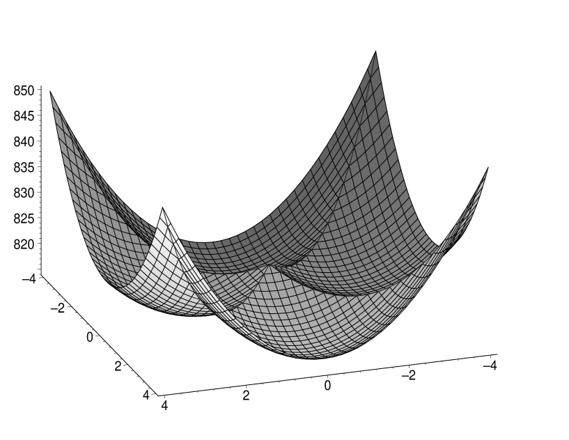
                       $\check{\sigma}_{2}$
                                                                                   $\check{\sigma}_{1}$

Figure 2: Diagram of the function $\check{V}_{\rm eff}(\check{\sigma}_{1},\check{\sigma}_{2})=V_{\rm eff}(\sigma_{1},\sigma_{2})/e^{6}$ at $H=40e^{3}$, $g_{1}=e^{-2}$, $g_{2}=20e^{-2}$. Here $\check{\sigma}_{1}=\sigma_{1}/e^{2}$, $\check{\sigma}_{2}=\sigma_{2}/e^{2}$.

Unfortunately, for the magnetic field such that $eHg_{i}^{2}\sim 1$ or $eHg_{i}^{2}\gg~{}1$, we were unable to prove this fact by means of the analytical technique. However, numerical calculations performed for a rather wide interval of values of $H$ confirm the above conclusion. For example, Fig. 2 depicts the function $V_{\rm eff}(\sigma_{1},\sigma_{2})$ at $H=40e^{3}$, $g_{1}=e^{-2}$, $g_{2}=20e^{-2}$ (here, evidently $eHg_{i}^{2}\gg 1$). In this case, the global minimum of the potential $\sigma_{1}=0$, $\sigma_{2}=2.77e^{2}$ corresponds to chiral symmetric phase of the model (parity is spontaneously broken).

It should also be remarked that an external magnetic field acting upon phases B and C (see Fig. 1) makes their ground states more stable. The fact is that there exists a rather strong fermion-antifermion attraction even at $H=0$ (at least one of the bare coupling constants $G_{i}$ is greater than $G_{c}$), leading to formation of one of the condensates $\bar{\psi}\psi$ or $\bar{\psi}\tau\psi$, i.e. to spontaneous breaking of the initial symmetry. An external magnetic field acts in favor of further increasing the condensate values, i.e. it stabilizes these phases. Since in these cases the magnetic field is not the cause (catalyzer) of the spontaneous symmetry breaking (a superstrong attraction of fermions and antifermions being the actual cause), details of these considerations are omitted. For completeness, however, the phase portrait of the model at arbitrary nonzero values of the external magnetic field and coupling constants $g_{1,2}$ is depicted in Fig. 3.

5 Conclusions

In the present paper, the influence of an external magnetic field on the 3-dimensional $P\times\Gamma_{5}$ symmetric model (1) is considered in the case, when bare coupling constants $G_{1,2}<G_{c}$ take sufficiently small values (positive values of constants $g_{1,2}$). The initial symmetry is unbroken, if $H=0$. Arbitrary small external magnetic field was shown to induce spontaneous breaking of $P\times\Gamma_{5}$ symmetry (phenomenon of magnetic catalysis). Moreover it turned out, that $P$ symmetry of the model is broken, while chiral symmetry remains intact, if $g_{2}>g_{1}$ (this is phase B of the theory). When $g_{1}>g_{2}$, the external magnetic field induces the second order phase transition from phase A to phase C, whose vacuum is $P$ symmetric, though having no chiral invariance.

6 Acknowledgments

The authors are grateful to D.Ebert for useful discussions. This work was partially supported by RFBR under grant number 98-02-16690, and by DFG, project DFG 436 RUS 113/477.

Appendix

Algebra of $\Gamma$-matrices for the 3-dimensional Lorentz group

Two-component Dirac spinors realize an irreducible 2-dimensional representation of the Lorentz group transformations of the 3-dimensional space-time. In this case, the $2\times 2$ matrices $\gamma$ have the form

$$\gamma^{0}=\sigma_{3}=\left(\begin{array}[]{cc}1&0\\ 0&-1\end{array}\right),\;\gamma^{1}=i\sigma_{1}=\left(\begin{array}[]{cc}0&i\\ i&0\end{array}\right),\;\gamma^{2}=i\sigma_{2}=\left(\begin{array}[]{cc}0&1\\ -1&0\end{array}\right).$$

These matrices have the properties

$$\mathop{\rm Tr}\nolimits(\gamma^{\mu}\gamma^{\nu})=2g^{\mu\nu};~{}~{}[\gamma^{\mu},\gamma^{\nu}]=-2i\varepsilon^{\mu\nu\alpha}\gamma_{\alpha};~{}~{}\gamma^{\mu}\gamma^{\nu}=-i\varepsilon^{\mu\nu\alpha}\gamma_{\alpha}+g^{\mu\nu},$$

where $g^{\mu\nu}=g_{\mu\nu}=\mathop{\rm diag}\nolimits(1,-1,-1),$ $\gamma_{\alpha}=g_{\alpha\beta}\gamma^{\beta},$ $\varepsilon^{012}=1$. Moreover,

$$\mathop{\rm Tr}\nolimits(\gamma^{\mu}\gamma^{\nu}\gamma^{\alpha})=-2i\varepsilon^{\mu\nu\alpha}.$$

Recently, one frequently exploits a reducible 4-dimensional representation of the Lorentz group, and the spinors $\psi_{k}$ from (1) transform according to this representation:

$$\psi=\left(\begin{array}[]{cc}\psi_{1}\\ \psi_{2}\end{array}\right).$$

In (A.4) $\psi_{1},\psi_{2}$ are two-component spinors. The gamma matrices that correspond to this representation have the form $\Gamma^{\mu}=\mathop{\rm diag}\nolimits(\gamma^{\mu},-\gamma^{\mu})$, where $\gamma^{\mu}$ are given in (A.1). It is easily demonstrated that ($\mu,\nu=0,1,2$):

$$\mathop{\rm Tr}\nolimits(\Gamma^{\mu}\Gamma^{\nu})=4g^{\mu\nu};~{}~{}\Gamma^{\mu}\Gamma^{\nu}=\sigma^{\mu\nu}+g^{\mu\nu};~{}~{}$$

$$\sigma^{\mu\nu}=\frac{1}{2}[\Gamma^{\mu},\Gamma^{\nu}]=\mathop{\rm diag}\nolimits(-i\varepsilon^{\mu\nu\alpha}\gamma_{\alpha},-i\varepsilon^{\mu\nu\alpha}\gamma_{\alpha}).$$

The dimensionality of the matrix algebra that acts in the four-dimensional spinor space is equal to 16, and its generators are $\Gamma^{\mu}$ $(\mu=0,1,2)$ and the matrix $\Gamma^{3}$ (anticommuting with them):

$$\Gamma^{3}=\left(\begin{array}[]{cc}0&I\\ I&0\end{array}\right),\;$$

where $I$ is a unit $2\times 2$ matrix. There exists one more matrix $\Gamma^{5}$, which anticommutes with all matrices $\Gamma^{\mu}$ and $\Gamma^{3}$:

$$\Gamma^{5}=i\left(\begin{array}[]{cc}0&-I\\ I&0\end{array}\right).$$

We note that matrix $\tau$ entering (1) has the form

$$\tau=\left(\begin{array}[]{cc}I&0\\ 0&-I\end{array}\right).$$

In the space of four-dimensional spinors (A.4), one can introduce the parity ($P$) and chiral $\Gamma_{5}$ transformations, those in terms of two-component spinors $\psi_{1,2}$ look like

$$P:~{}\psi_{1k}(t,x,y)\longrightarrow\gamma^{1}\psi_{2k}(t,-x,y),~{}~{}~{}\psi_{2k}(t,x,y)\longrightarrow\gamma^{1}\psi_{1k}(t,-x,y),$$

$$\Gamma_{5}:~{}\psi_{1k}(t,x,y)\longrightarrow-i\psi_{2k}(t,x,y),~{}~{}~{}\psi_{2k}(t,x,y)\longrightarrow i\psi_{1k}(t,x,y).$$

Discrete transformations (A.8) can be easily rewritten with the use of the four-component spinors (A.4)

$$P:~{}\psi(t,x,y)\rightarrow i\Gamma^{1}\Gamma^{5}\psi(t,-x,y);~{}~{}~{}~{}\Gamma_{5}:~{}\psi\rightarrow\Gamma^{5}\psi.$$

Figure 1: Phase portrait of the model in terms of $g_{1}$ and $g_{2}$ at $H=0$. Here $l=\{(g_{1},g_{2})~{}:~{}g_{1}=g_{2}\}.$

          $\check{V}_{\rm eff}(\check{\sigma}_{1},\check{\sigma}_{2})$

Figure 3: Phase portrait of the model in terms of $g_{1}$ and $g_{2}$ at $H\not=0$. Line $l$ defined on Fig. 1.

References

• [1] D.J. Gross and A. Neveu, Phys. Rev. D 10, 3235 (1974).
• [2] K.G. Klimenko, Theor. Math. Phys. 89, 1161 (1992); Theor. Math. Phys. 90, 1 (1992); K.G. Klimenko, Z. Phys. C 54, 323 (1992).
• [3] I.V. Krive and S.A. Naftulin, Phys. Rev. D 46, 2737 (1992).
• [4] V.P. Gusynin, V.A. Miransky and I.A. Shovkovy, Phys. Rev. Lett. 73, 3499 (1994); Phys. Rev. D 52, 4718 (1995); V.P. Gusynin and I.A. Shovkovy, Phys. Rev. D 56, 5251 (1997); A.Yu. Babansky, E.V. Gorbar and G.V. Shchepanyuk, Phys. Lett. B 419, 272 (1998).
• [5] K.G. Klimenko, A.S. Vshivtsev and B.V. Magnitsky, Nuovo Cim. A 107, 439 (1994); A.S. Vshivtsev, K.G. Klimenko and B.V. Magnitsky, Theor. Math. Phys. 101, 1436 (1994); Phys. Atom. Nucl. 57, 2171 (1994).
• [6] A.S. Vshivtsev, V. Ch. Zhukovsky, K.G. Klimenko and B.V. Magnitsky, Phys. Part. Nucl. 29, 523 (1998).
• [7] I.A. Shovkovy and V.M. Turkowski, Phys. Lett. B 367, 213 (1995); D. Ebert and V.Ch. Zhukovsky, Mod. Phys. Lett. A 12, 2567 (1997); V.P. Gusynin, D.K. Hong and I.A. Shovkovy, Phys. Rev. D 57, 5230 (1998).
• [8] G.W. Semenoff, I.A. Shovkovy and L.C.R. Wijewardhana, Phys. Rev. D 60, 105024 (1999).
• [9] W.V. Liu, Nucl. Phys. B 556, 563 (1999).
• [10] T. Inagaki, T. Muta and S.D. Odintsov, Progr. Theor. Phys. Suppl. 127, 93 (1997); E.J. Ferrer and V. de la Incera, Int. J. Mod. Phys. 14, 3963 (1999); Phys. Lett. B 481, 287 (2000); E.J. Ferrer and V. de la Incera, On magnetic Catalysis and Gauge Symmetry Breaking, hep-th/9910035; V. de la Incera, hep-ph/0009303.
• [11] K. Farakos and N.E. Mavromatos, Int. J. Mod. Phys. B 12, 809 (1998); K. Farakos, G. Koutsoumbas and N.E. Mavromatos, Int. J. Mod. Phys. B 12, 2475 (1998); N.E. Mavromatos and A. Momen, Mod. Phys. Lett. A 13, 1765 (1998); G.W. Semenoff, I.A. Shovkovy and L.C.R. Wijewardhana, Mod. Phys. Lett. A 13, 1143 (1998).
• [12] V.A. Miransky, Progr. Theor. Phys. Suppl. 123, 49 (1996); V.P. Gusynin, Magnetic Catalysis of Chiral Symmetry Breaking in Gauge Theories, hep-th/0001070.
• [13] A.S. Davydov, Phys. Rep. 190, 191 (1990).
• [14] K. Krishana et al, Science, 277, 83 (1997).
• [15] G.W. Semenoff and L.C.R. Wijewardhana, Phys. Rev. Lett. 63, 2633 (1989); Phys. Rev. D 45, 1342 (1992).
• [16] M. Carena, T.E. Clark and C.E.M. Wagner, Phys. Lett. B 259, 128 (1991); // Nucl. Phys. B 356, 117 (1991).
• [17] B. Rosenstein, B.J. Warr and S.H. Park, Phys. Rep. 205, 59 (1991).
• [18] K.G. Klimenko, Z. Phys. C 57, 175 (1993); Teor. Mat. Fiz. 95, 42 (1993).
• [19] A.P. Prudnikov, U.A. Brychkov, O.I. Marichev, Integrals and series (in Russian), Moscow: Nauka, 1974.
• [20] E.T. Whittaker and G.N. Watson, A Course of Modern Analysis, Vol. 2, Cambridge: University Press, 1927.
• [21] E. Elizalde, S. Leseduarte, S.D. Odintsov and Yu.I. Shilโ€™nov, Phys. Rev. D 53, 1917 (1996); D.M. Gitman, S.D. Odintsov and Yu.I. Shilโ€™nov, Phys. Rev. D 54, 2964 (1996); A.S. Vshivtsev, K.G. Klimenko and B.V. Magnitsky, Theor. Math. Phys. 106, 319 (1996); JETP Lett. 62, 283 (1995); T. Inagaki, S.D. Odintsov and Yu.I. Shilโ€™nov, Int. J. Mod. Phys. A 14, 481 (1999).
• [22] K. G. Klimenko, Z. Phys. C 37, 457 (1988); D. Y. Song, Phys. Rev. D 48, 3925 (1993); S.J. Hands, A. Kocic and J.B. Kogut, Ann. Phys. 224, 29 (1993); Kanemura and H.-T. Sato, Mod. Phys. Lett. A 11, 785 (1996); M. Modugno, G. Pettini and R. Gatto, Phys. Rev. D 57, 4995 (1998); B.-R. Zhou, Phys. Lett. B 444, 455 (1998); G. Miele and P. Vitale, Nucl. Phys. B 494, 365 (1997); P. Vitale, Nucl. Phys. B 551, 490 (1999); D.K. Kim and K.G. Klimenko, J. Phys. A 31, 5565 (1998); L. Rosa, P. Vitale and C. Wetterich, hep-th/0007093; T. Appelquist and M.Schwetz, hep-ph/0007284.
$g_{2}$ $g_{1}$Phase A$\langle\sigma_{1}\rangle=0,~{}\langle\sigma_{2}\rangle=0$Phase BPhase BโŸจฯƒ1โŸฉ=0,โŸจฯƒ2โŸฉโ‰ 0formulae-sequencedelimited-โŸจโŸฉsubscript๐œŽ10delimited-โŸจโŸฉsubscript๐œŽ20\langle\sigma_{1}\rangle=0,~{}\langle\sigma_{2}\rangle\not=0Phase CPhase CโŸจฯƒ1โŸฉโ‰ 0,โŸจฯƒ2โŸฉ=0formulae-sequencedelimited-โŸจโŸฉsubscript๐œŽ10delimited-โŸจโŸฉsubscript๐œŽ20\langle\sigma_{1}\rangle\not=0,~{}\langle\sigma_{2}\rangle=0$l$