In this note we address the issue of theoretical estimates of the hadronic cross-sections for $\gamma\gamma$ processes. We compare the predictions of the minijet model with data as well as other models, highlighting the band of uncertainties in the theoretical predictions as well as those in the final values of the $\sigma(\mbox{$\gamma\gamma$}\rightarrow{\rm hadrons})$ extracted from the data. We find that the rise of $\sigma_{\gamma\gamma}^{\rm tot}$ with energy shown in the latest $\gamma\gamma$ data is in tune with the faster rise expected in the Eikonal Minijet Models (EMM). We present an estimate of the accuracy with which this cross-section needs to be measured, in order to distinguish between the different theoretical models which try to ‘explain ’ the rise of total cross-sections with energy. We find that the precision of measurement required to distinguish the EMM type models from the proton-like models, for $300<\sqrt{s}_{\mbox{$\gamma\gamma$}}<500$ GeV, is $\>\raisebox{-2.15277pt}{$\stackrel{{\scriptstyle\textstyle<}}{{\sim}}$}\>20\%$, whereas to distinguish between various proton-like models or among the different parametrizations of the EMM, a precision of $\>\raisebox{-2.15277pt}{$\stackrel{{\scriptstyle\textstyle<}}{{\sim}}$}\>8-9\%$ or $\>\raisebox{-2.15277pt}{$\stackrel{{\scriptstyle\textstyle<}}{{\sim}}$}\>6-7\%$ respectively, is required. We also comment briefly on the implications of these predictions for hadronic backgrounds at the next linear collider (NLC) to be run in the $\gamma\gamma$ mode or $e^{+}e^{-}$ mode.

1 Introduction

The rising total cross-section in proton-proton collisions was a very early indication of QCD processes at work, reflecting the fact that the increasing energy allows for deeper and deeper probe of the structure of the colliding particles[1] leading to liberation of more and more constituents, resulting in higher scattering probability. The proton-proton and proton-antiproton cross-sections are now known experimentally to a very good precision. We do not yet fully understand these cross-sections from first principles, but there are various models of hadronic interactions whose parameters can be completely fixed by the data and which then allow for good predictions of the total cross-section in the high energy region, certainly up to LHC energies. Thus, although not everything is calculable from first principles in QCD, there is no problem as far as predicting the total hadronic production at future accelerators is concerned. The situation is substantially different for the photon induced processes. This renders the issue of measurement of the total $\gamma\gamma$ cross-section at energies in the region 300-500 GeV range very important both from the theoretical point of view, as well as experimental. Indeed,the question of hadron production in $\gamma\gamma$ collisions is interesting from a point of view of achieving a good theoretical understanding of the rise of the hadronic cross-sections with energy, in the framework of QCD or otherwise, as well as from a much more pragmatic viewpoint of being able to estimate the hadronic backgrounds at the next linear colliders [2]. There exist two classes of models which have been suggested in the context of rise of the hadronic cross-sections in $pp$ and $\bar{p}p$ processes. All of these ‘explain’ the rise for the $pp$ and $\bar{p}p$ case equally well but differ greatly in their predictions for $\gamma\gamma$ collisions even at the modest values of the $\gamma\gamma$ energies that are currently available. HERA and LEP have opened the way to an entire new field in QCD, the study of the hadronic interactions of the photon in terms of its quark and gluon content [3]. Hadronic collisions show the beginning of the rise to take place at centre of mass energies below 100 GeV but to determine the steepness of the rise one needs points in the 300-500 GeV and even higher. Thus, as in the case of hadron collisions, to gain a good theoretical understanding of the total cross-section for $\gamma\gamma$ processes, one needs much higher energies and better statistics than the one currently available from LEP and HERA. At LEP phase space limits the c.m. energy of the $\gamma\gamma$ system to about 100 GeV, at HERA $\sqrt{s}_{\gamma p}$ is higher, but then the presence of proton partly obscures the issue. Note that, until five years ago, the available data for $\gamma\gamma$  processes did not yet show any rise, stopping short of $\sqrt{s}=20$ GeV and with very large errors. L3 and OPAL data have drastically changed the situation. Presently, the $\gamma\gamma$  cross-section data show a very clear rise, but there are a number of theoretical and experimental issues, which only the Linear Collider(LC) can clarify, by reaching higher energies and statistics. In what follows we shall discuss the theoretical issues which can only be resolved by measurements of total cross-sections at higher and higher energies in the $\gamma\gamma$ system. In this note we first discuss predictions [4] for $\sigma(\mbox{$\gamma\gamma$}\ \to{\rm hadrons})$, in the Eikonal Minijet Model (EMM), and then make a comparison with other models as well as the presently available experimental data, contrasting the uncertainties in the model predictions with those in the values of $\sigma(\mbox{$\gamma\gamma$}\ \to{\rm hadron})$ extracted from the existing two-photon data [5, 6, 7].

2 QCD and total cross-sections

QCD predicts the rise of total cross-sections through the increasing number of gluon-gluon collisions. For this, one can take the approach of the BFKL equation, which resums all the QCD diagrams, using a frozen value of $\alpha_{s}$ for the final evaluation, the underlying idea being that both the decrease, ”Regge type” behaviour, as well as the rise, i.e. the ”Pomeron” like behaviour are QCD effects. The calculation gives imaginary part of all the summed diagrams and hence the total cross-section. This method does not yet allow for a precision estimate. Hence, while from a theoretical point of view this is fundamentally the correct approach to follow, at present it does not have much predictive power. A different, more pragmatic approach is the one of the EMM[8], which uses the eikonal approximation to calculate the elastic amplitude and hence the imaginary part, i.e. the total cross-section, and the QCD jet cross-section drives the rise with energy. Notice that the eikonal approximation is indeed just an approximation and hence has its inherent limitations. The neglected terms can, in principle, play a non-negligible role. The interest in using the Mini-jet Model[9] (we will discuss the details of the model later) lies in the fact that the phenomenological triumphs of QCD are based on the possibilty of predicting the jet cross-sections in terms of a set of basic parton processes and parton densities parametrizing the parton distributions in the proton or in the photon. Hence, it is this aspect of QCD which can be put to trial in calculating the rise of total cross-sections using the EMM approach, viz. the validity of our description of the scattering processes through the above two ingredients. Since we are dealing with a total cross-section, it is only the inclusive jet yield given by

$$\sigma^{\rm jet}(s,p_{\rm tmin})=\int_{p_{\rm tmin}}d^{2}{\vec{p}_{t}}{{d\sigma_{jet}}\over{d^{2}{\vec{p}_{t}}}}.$$ (1)

which enters into the calculation. Here ${{d\sigma_{jet}}/{d^{2}{\vec{p}_{t}}}}$, is the differential jet cross-section calculated using QCD. This result depends upon the minimum jet transverse momentum used in the calculation and the choice of parton densities for the hadron. For the case of the photon the available parametrizations in the low-x region differ from each other substantially.

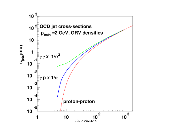
Figure 1: Integrated jet cross-sections for $p_{\rm tmin}=2\ GeV$.

In Fig.1 we show the minijet cross-section defined by eq. 1 for three different types of processes viz., proton-proton, photon-proton and photon-photon interactions. Of course, in order to be able to compare all of them together, we have normalized them, by a multiplication with an appropriate power of $\alpha$, the fine structure constant. In this figure we have chosen $p_{\rm tmin}=2\ GeV$, a rather conservative value, based upon various phenomenological attempts at fitting $\sigma^{\rm tot}$ in different cases. In both the cases where photon is one of the colliding particles, two types of processes contribute to the jet cross-sections: the ‘resolved’ processes, in which partons in the photon participate in the hard scattering process producing the jets and the ‘direct’ processes in which a photon participates directly in the ‘hard’ subprocess generating the final state jets. This accounts for part of the difference between the three curves. Another important difference is the markedly harder $x$-dependence of the quark densities in the photon reflecting the hard nature of the $q\bar{q}\gamma$ vertex, which gives rise to the perturbative part of the photonic quark densities. In the region where the gluon content is expected to dominate, the three curves superimpose as they should. In this figure we have chosen the GRV[10] densities for protons as well as for the photons. However, the general features we mention are insensitive to our choice of the photonic densities. The rise of the (mini)jet cross-sections with $\sqrt{s}$ is however too steep for any fixed $p_{\rm tmin}$ value, and these cross-sections need to be incorporated in a theoretical framework which preserves unitarity, to allow for the calculation of a total cross-section. The eikonal formulation provides a framework in which the minijet cross-sections are unitarised via multiple scattering [11]. Let us write down, very briefly, the formulation of the EMM for the $pp/\bar{p}p$ case. The starting point is the eikonal formulation for the elastic scattering amplitude.

$$f(\theta)={{ik}\over{2\pi}}\int d^{2}{\vec{b}}e^{i{\vec{q}}\cdot{\vec{b}}}[1-e^{i\chi(b,s)}]$$ (2)

Along with the optical theorem this leads to the expression for the total cross-sections

$$\sigma^{\rm el}_{pp(\bar{p})} = \int d^{2}{\vec{b}}|1-e^{i\chi(b,s)}|^{2}$$ (3)

$$\sigma^{\rm tot}_{pp(\bar{p})} = 2\int d^{2}{\vec{b}}[1-e^{-\chi_{I}(b,s)}cos(\chi_{R})]$$ (4)

$$\sigma^{\rm inel}_{pp(\bar{p})} = \sigma^{\rm tot}-\sigma^{\rm el}=\int d^{2}{\vec{b}}[1-e^{-2\chi_{I}(b,s)}]$$ (5)

The jet cross-section is a priori an inelastic part of the total cross-section, and thus is used as an input to the eikonalized formulation of the inelastic cross-section. The eikonal formulation introduces a new set of uncertainties in this calculation, viz. the impact parameter distribution in the colliding particles, a semi-classical concept, whose range of validity is limited to the large b-collisions. The arbitrariness introduced by this function needs to be evaluated carefully. It plays a role not only in the low energy behaviour, but also, and very much so, in the rise. It is possible to relate this function to QCD processes, and attempts to calculate it have been partially successful[12]. Of course, the rise with energy is only one of the phenomenological aspects of total cross-sections. Hence one should expect the function $\chi_{I}(b,s)$ to have both a soft part which is nonperturbative in origin and cannot be calculated in this context, and a ‘hard’ component which can be. A useful working scheme is one in which one breaks down the eikonal function in a number of building blocks, and then examines their phenomenological implications, varying the input parameters in each one of them. To be concrete, we write

$$2\chi_{I}(b,s)=n_{\rm soft}(b,s)+n_{\rm PQCD}(b,s)$$ (6)

with

$$n_{\rm soft}(b,s)=A_{s}(b,s)\sigma^{\rm soft}(s)$$ (7)

and

$$n_{\rm PQCD}(b,s)=A_{h}(b,s)\sigma^{\rm jet}(s,p_{\rm tmin})$$ (8)

Here $\sigma_{\rm jet}$ is given by eq. 1. This breakdown uses the assumption of factorization into the transverse and longitudinal degrees of freedom, in other words between the impact parameter distribution and the energy dependence. In this paper we have fitted the data using a further approximation:

$$2\chi_{I}(b,s)\equiv n(b,s)=A(b)[\sigma^{\rm soft}(s)+\sigma^{\rm jet}(s,p_{\rm tmin})]$$ (9)

viz. assuming the same impact parameter distribution function for soft and hard processes. In addition we have also assumed independence of the overlap function on $s$. This approximation may be too rough, but, lacking a full theoretical description for this function, we prefer to study the energy behaviour only through the hard cross-section, and modify this assumption only later. Note that $\sigma_{jet}$ can be calculated completely in perturbative QCD once we have the knowledge of parton densities in the hadrons involved. For the case of photon induced processes, the above formulation needs to be generalised [13]to include the probability that photon behaves like a hadron in the collision. This generalisation has been implemented in the earlier analyses of $\sigma^{\rm inel}_{\gamma p}$  [14, 15]. We denote this probability by $P^{\rm had}_{\rm ab}$, which is unity for hadron-hadron (denoted by a,b) processes, but of order $\alpha_{\rm em}$ or $\alpha_{\rm em}^{2}$ for processes where one or both of the hadrons participating in the collisions are photons. Using Vector Meson Dominance (VMD), and a running $\alpha_{\rm em}$, this parameter varies from 1/250 at $\sqrt{s}=5$ GeV to 1/240 at $\sqrt{s}=300$ GeV. The generalisation involves putting the factor $P^{\rm had}_{\rm ab}$ on the R.H.S. in eqs. 4, 5 and dividing the second term in the square bracket in eq. 9 by the same factor. Of course the $p$ in the subscripts will get changed to $\gamma$ depending on the number of photons involved in the initial state. The definition of $\sigma^{\rm soft}$ in eq.9 is such that, even in the photonic case, it is of hadronic size. Hence only the second term in the square bracket of eq. 9 gets the factor of $P_{\rm ab}^{\rm had}$. A simple way to understand the need for this factor [13] is to realise that the unitarisation in this formalism is achieved by multiple parton interactions in a given scatter of hadrons and once the photon has ‘hadronised’ itself, one should not be paying the price of $P_{\gamma}^{\rm had}$ for further multiparton scatters. The eikonalised cross-sections depend only on a particular combination of the hadronic factor $P^{\rm had}_{\rm ab}$ and the impact parameter distribution function $A_{ab}(b)$. This, together with the simple scaling properties of the eikonal formulation, allows for an interesting graphical description of the b-distribution in the three different cases of proton-proton, $\gamma\$proton and photon-photon collisions. On dimensional grounds, the function $A_{ab}(b)$ in general depends on two scale parameters, describing respectively the matter distribution in the two colliding particles a and b. Denoting such parameters by $k_{a}$ and $k_{b}$, where $a,b=\gamma$ or $proton$, and assuming that the matter distribution in b-space factorizes into the Fourier transform of the electromagnetic form factor of the colliding particles, we have

$$A_{ab}(b)\equiv A(b;k_{a},k_{b})={{1}\over{(2\pi)^{2}}}\int d^{2}{\vec{q}}e^{iq\cdot b}{\cal F}_{a}(q,k_{a}){\cal F}_{b}(q,k_{b})$$ (10)

$$\equiv{{1}\over{(2\pi)^{2}}}\int d^{2}{\vec{q}}e^{iq\cdot b}{\cal F}_{a}(q/k_{a}){\cal F}_{b}(q/k_{b})$$ (11)

The general expression of the inelastic cross-section now reads

$$\sigma^{inel}_{ab}=P^{\rm had}_{\rm ab}\int d^{2}{\vec{b}}[1-e^{-n(b,s)}]$$ (12)

To see the effect of $P^{\rm had}_{\rm ab}$ on the b-distribution, we scale out the factor $P^{\rm had}_{\rm ab}$, obtaining

$$\sigma^{inel}_{ab}=\int d^{2}{\vec{b}}[1-e^{-{\bar{A}}(b;{\tilde{k}}_{a},{\tilde{k}}_{b})[P^{\rm had}_{\rm ab}\sigma^{soft}+\sigma^{jet}]}]$$ (13)

with ${\bar{A}}(b;{\tilde{k}}_{a},{\tilde{k}}_{b})=A(b;{\tilde{k}}_{a},{\tilde{k}}_{b})/P_{ab}^{\rm had}$ where ${\tilde{k}}_{a/b}=k_{a/b}/\sqrt{P^{\rm had}_{\rm ab}}$. With this, all three total/inelastic cross-sections, $p\ p/{\bar{p}}$, $\gamma\ p$ and $\gamma\gamma$ can be obtained from the same expression, with different overlap functions.

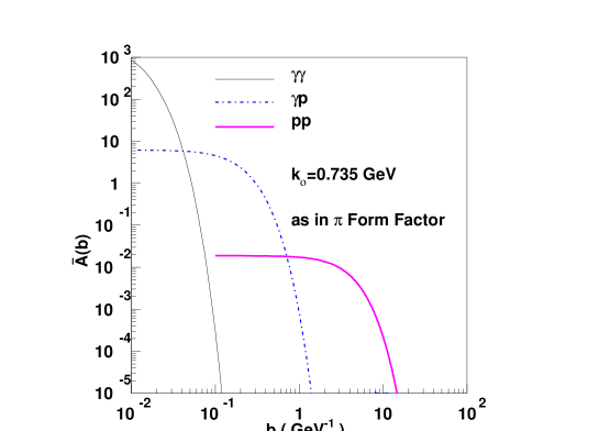
Figure 2: The impact parameter distribution for protons and photons

To see the effects of these differences between photons and protons [16], we have plotted in Fig.2 the function ${\bar{A}}(b;{\tilde{k}}_{a},{\tilde{k}}_{b})$, for the case of $P^{\rm had}_{\gamma p}=1/240$, using the usual dipole function for the proton form factor and the pion form factor for the photon. This figure graphically emphasizes the difference in spatial extension between photons and protons.

For calculations, we revert to eq.(12), which, in the above eikonal formulation, very clearly defines the inelastic cross-section. Making the further approximation, well borne by experiment, that the real part of the eikonal $\chi_{R}(b,s)$ is zero, one is in principle ready to fit the data for the total photon-photon cross-sections, using

$$\sigma^{tot}_{ab}=2P^{\rm had}_{\rm ab}\int d^{2}{\vec{b}}[1-e^{-n(b,s)/2}]$$ (14)

The strategy adopted in [4] consisted in determining the various parameters, $\sigma^{\rm soft},P_{\gamma p}^{\rm had},k_{\rm proton},k_{\gamma},p_{\rm tmin}$ and the choice of photon densities, using the process $\gamma p$ and then, predict cross-sections for $\gamma\gamma$. Next, for those parameters/functions which are non perturbative and need to be modified, we use factorisation; viz. $P_{\gamma\gamma}^{\rm had}=[P_{\gamma p}^{\rm had}]^{2}$ and the Quark Parton Model, i.e. $\sigma^{\rm soft}_{\gamma\gamma}={{2}\over{3}}\sigma^{\rm soft}_{\gamma p}$. For the hard part of the eikonal, we keep the same photonic parton densities, $p_{\rm tmin}$, and $k_{\gamma}$ as in the $\gamma p$ case. Note that the value of $k_{\gamma}$ used in [4] corresponds to a different ansatz in the case of photonic partons than the one mentioned in the discussion above. In [4] we have taken the matter distribution to be the Fourier Transform of the transverse momentum distribution. Technically it only means using the experimentally measured value of $k_{\gamma}$, that is $0.66\pm 0.22$ [17], instead of the value of $0.735$ used, for illustration, in Fig. 2. The correlated predictions of the EMM for $\gamma p$ and $\gamma\gamma$ have been discussed in [18]. The resulting curves for $\gamma\gamma$ total cross-section are shown in

Figure 3: Predictions of the EMM for different densities

Fig.3 for three different sets of parton densities [10, 19, 20] and compared with data for $\sqrt{s}=189$ GeV, from the L3[6] and OPAL [5] Collaborations respectively. We have chosen a set of parameters which give compatible fits to both the HERA[21, 22] and the LEP data. It should be noted that all these curves give predictions which lie below the L3 data extracted with Pythia Monte Carlo [6]. The most recent data analysis by the L3 Collaboration, inclusive of $202$ GeV data [7], obtained averaging between Pythia and Phojet, is now in full agreement with the OPAL data. At the same time, recently, new data for the $\gamma p$ cross-sections, extracted from Deep Inelastic Scattering have appeared[23], and new photoproduction data should be available soon. Thus complete reliance on the extrapolation from $\gamma p$ is not yet advisable. A 10% change of the parameters of the EMM prediction, for instance, can now give a very good agreement with the present data, as we show in Fig.4, where,

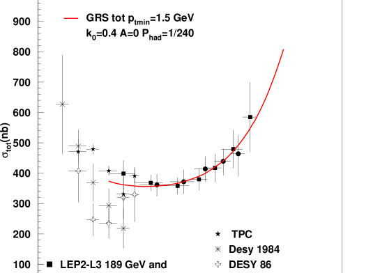
Figure 4: EMM description of present $\gamma\gamma$ total cross-section, with parameters extracted from $\gamma p$ with 10% changes as indicated in the text.

to obtain this figure, we have followed the procedure described above, except that the value for the photon intrinsic transverse momentum $k_{\gamma}$ used is $0.4$ GeV which is lower than the $k_{\gamma}=0.66$ GeV, i.e. the central value of $k_{\gamma}$ given by experiment [17] and which produces good fits of the EMM predictions to the published photoproduction data on $\sigma^{\rm tot}_{\gamma p}$[21, 22]. The other relevant parameters are

$$P^{\rm had}_{\gamma p}\equiv P_{\rm had}={{1}\over{240}}\ ;\ \ \ \ \sigma^{soft}=\sigma_{0}+{{\cal B}\over{s}}\ ;\ \ \sigma_{0}=20.8\ mb\ ;\ {\cal B}=42.1{{mb}{{\rm GeV}^{2}}}$$ (15)

All the minijet curves we have shown indicate a rather steep rise of the total cross-section. There exist however other predictions, which one could call “proton-like” predictions, which reflect the validity of factorization for total cross-sections at present energies and in which the predicted rise at high energy is very different from the Eikonalised Minijet Model. This is the case of the Aspen Model[24], in which both the rise and the shape of the $b-$distribution are derived from the proton with simple scaling properties. Although at very high energies this may not be true, at present energies this model satisfies the factorization hypothesis $\sigma_{\rm nn}=\sigma_{\gamma p}^{2}/\sigma_{\gamma\gamma}$[25]. Another “proton-like” model is the Regge-Pomeron exchange model, in which factorization (at the residues) holds independently for the low (Regge) energy and the high (Pomeron) energy term. Most of the “proton-like” models have the same high energy rise in all the three $pp$,$\gamma\ p$ and $\gamma\gamma$ cross- sections, as typified by the Regge-Pomeron exchange model, where $\sigma^{tot}\approx s^{\epsilon}$, with $\epsilon=0.08$[26]. There is a priori no justification in these models for a change in curvature from hadrons to photons, although data have recently been parametrized with different values of the Pomeron intercept parameter $\epsilon$. On the other hand, the different rate at which $\sigma$ rises with energy in the other models has, obviously, both theoretical and experimental implications. The latter because, as shown later, the predictions of different models can differ by a factor 2 or 3 at the values of energy of interest to NLC and since these cross-sections enter in the calculations of photon-induced hadronic background, the corresponding error in the prediction is then quite large. But even more important is the issue of arriving at a theoretical understanding of these differences and resolution as to which is theoretically more satisfactory and trustworthy. It is also worthwhile to determine whether the faster rise in minijet models is to be traced to the extrapolated low-x behaviour of the parton densities or is it inherent to the eikonal model. An understanding of how a different curvature can arise, in principle, can be obtained from the EMM model. As shown in Fig.1, at high energy the minijet cross-sections, obtained from gluon-gluon scattering, all rise with the same slope. However, their convolution with different impact parameter distributions changes the pattern. To see this, we

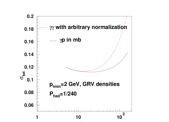
Figure 5: Comparison of the energy dependence of the EMM predictions for the total $\gamma\gamma$ and $\gamma p$ cross-sections with $p_{\rm tmin}=2$ GeV, $P_{\rm had}=1/240.$

plot in Fig.5 the EMM curve for $\gamma p$ and the one for $\gamma\gamma$, obtained with the same set of parameters. We have normalized the two curves in the low energy region, where they can be brought to coincide, thus confirming factorization at low energy. As the mini-jet cross-section starts rising, and multiple scattering plays a role, then the differences between the impact parameter distributions, dipole for the proton or monopole for the photon, become important and the two curves do not coincide anymore.

To complete the description of existing models for the $\gamma\gamma$ cross-sections, we would like to address the question of whether data and models are actually looking at the same quantity; viz. the question of Total versus Inelastic Cross-sections in photon induced processes.

For photon induced processes, the issue of total cross-section is ill defined both theoretically and experimentally. In this case, the $\gamma p$($\gamma\gamma$) cross-sections are extracted from a measurement of the $ep(e^{+}e^{-})$ processes. These cross-sections therefore depend on the acceptance corrections that have to be employed. These in turn are strongly influenced by the Monte Carlo models to describe different components of an event. For example, the extraction of $\sigma_{\gamma p}^{\rm tot}$ needs understanding of three different kinds of events: (i) quasi-elastic process $\gamma p\to Vp$, where the proton remains intact and the photon gets transformed into a vector meson, (ii) diffractive where the proton and/or the photon break up but no colour exchange takes place and (iii) the nondiffractive where both the proton and $\gamma$ break up and colour is exchanged between the two. In case of $\gamma\gamma$ cross-sections, there are three different kinds of contributions; (i) the soft interactions modelled by VDM ideas. These have an exponential $p_{T}$ spectrum (ii) the direct interactions of the photon which can be estimated using the Quark Parton Model (QPM) and (iii) the resolved contributions which rise from the partons in the photon. Let us note that the first contribution is not to be confused with the nonperturbative part of the photon structure function. VDM ideas are sometimes used to estimate this part. These VDM partons also take part in the hard, resolved interactions which are used in calculating $\sigma_{\gamma p}^{\rm jet}$/ $\sigma_{\gamma\gamma}^{\rm jet}$ in the EMM. So again the extraction of $\sigma_{\mbox{$\gamma\gamma$}}$ from the $e^{+}e^{-}$ data involves a clear understanding of all these types of events. The soft interactions of type (i) are what can be losely termed as ‘elastic’ cross-section in this case. Thus we see that both theoretically and experimentally the ideas about elastic/total cross-section are ill defined in the case of photon induced processes.

In the earliest applications of the EMM model to the photons [14, 15], the inelastic formulation was used. This is correct if the hadrons in the final state can be defined as all of inelastic origin, i.e. no vector meson decays, for instance. Then, fixing the parameters for the EMM from a fit of the inelastic $\gamma p$ cross-section to the data, one can extrapolate to the $\gamma\gamma$ case, and obtain the prediction for the inelastic $\gamma\gamma$ cross-section. This procedure would produce a curve which rises less steeply than the one shown in Fig.4. On the other hand, as discussed first in  [24] and as has been discussed above, if the data have correctly included all the diffractive ”elastic” processes, then the quantity to be compared with the available data should be the ‘total’ cross-sections of eq. 3 and not the inelastic one. If we use the ‘total’ cross-section formulation using the eqs. 3- 5, use the known inputs for the parton densities from the photon structure function measurements and further fix the unknown ad-hoc parameter $p_{T}^{\rm min}$ of the EMM using the data from $\sigma^{\rm tot}_{\gamma p}$, we then get the predictions given in Fig. 3. If we do the same using the inelastic formulation, then we get a curve which at lower energies is higher, but then rises less fast.

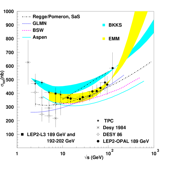
Figure 6: The predictions from from factorization models, Regge-Pomeron exchange and a QCD structure function models together with those from the EMM and a comparison with present data.

In Fig.6 we have plotted the recent data from LEP and from lower energies with the predictions from “proton-like” models, labelled SaS[19], Aspen[24], BSW[25], as well as from QCD and Regge inspired models, like the curve labelled GLMN[28] and the band labelled BKKS[27]. The band labelled EMM corresponds to the two formulations, inelastic and total. For the EMM, we have used two sets of representative parameters, both of which are obtained from the $\gamma p$ cross-section following the procedure outlined in [4].

3 Precision necessary

In this section we show the numerical values corresponding to various predictions for the total $\gamma\gamma$ cross-section and indicate the precision needed to distinguish among these different models[29].

Table 1: Precision required for the measurement of $\gamma\gamma$ cross-sections to distinguish between the different ‘proton’ like models

$\sqrt{s_{\gamma\gamma}}(GeV)$	Aspen	BSW	DL	$1\sigma$
20	309 nb	330 nb	379 nb	7%
50	330 nb	368 nb	430 nb	11%
100	362 nb	401 nb	477 nb	10%
200	404 nb	441 nb	531 nb	9%
500	474 nb	515 nb	612 nb	8%
700	503 nb	543 nb	645 nb	8%

In Table  1 we show total $\gamma\gamma$ cross-sections for three models of the ‘proton-is-like-the-photon’ type. The last column shows the 1$\sigma$ level precision needed to discriminate between Aspen[24] and BSW[25] models. The model labelled DL is obtained from Regge/Pomeron exchange with parameters from ref.[26] and factorization at the residues. The difference between DL and either Aspen or BSW is bigger than between Aspen and BSW at each energy value. A similar table can be drawn for distinguishing between the two minijet formulations of Fig.6 and the BKKS model[27], for instance.

Table 2: Precision required for the measurement of $\gamma\gamma$ cross-sections to distinguish between different formulations of the EMM and BKKS [27]

$\sqrt{s_{\gamma\gamma}}(GeV)$	EMM, Inel,GRS	EMM, Tot,GRV	BKKS	$1\sigma$
	($p_{\rm tmin}$=1.5 GeV)	($p_{\rm tmin}$=2 GeV)	GRV
20	399 nb	331 nb	408 nb	2 %
50	429 nb	374 nb	471 nb	9%
100	486 nb	472 nb	543 nb	11%
200	596 nb	676 nb	635 nb	6%
500	850 nb	1165 nb	792 nb	7 %
700	978 nb	1407 nb	860 nb	13 %

The last column in Table 2 now gives the percentage difference between the two models which bear closest results, i.e. EMM with GRS densities and inelastic formulation on the one hand and BKKS, as well as EMM with GRV densities and total formulation on the other.

4 The hadronic backgrounds at Linear Colliders

Apart from the above mentioned theoretical interest in studying the $\gamma\gamma$ cross-sections, a very pragmatic reason is the hadronic backgrounds that the beamstrahlung effects might cause at these colliders. One way to estimate that is to look at the quantity $\sigma^{\rm jet}_{\mbox{$\gamma\gamma$}}$ defined in eq. 1. While it is true that only part of the rise with $\sqrt{s}$ of $\sigma(\gamma\gamma\rightarrow{\rm jets})$ is reflected in the energy dependence of $\sigma^{\rm inel}$, the quantity is still a good measure of the messiness caused by the hadronic backgrounds at the NLC due to beamstrahlung. Here we give a new parametrisation of the ‘minijet’ cross-sections in $\gamma\gamma$ collisions which can be used in estimating the hadronic backgrounds at the NLC’s by folding it with appropriate beamstrahlung spectra. This supercedes the corresponding parametrisation that was given in [30].

The ’minijet’ cross-section, for the two parametrisations GRV [10] and SAS [19] densities, is given (in nb)

$$\sigma_{minijet} = \left[222\left({2\;{\rm GeV}\over\mbox{$p_{\rm tmin}$}}\right)^{2}-161\left({2\;{\rm GeV}\over\mbox{$p_{\rm tmin}$}}\right)+36.6\right]\left({\sqrt{s}\over 50}\right)^{1.23}$$ (16)

$$= \left[77.6\left({2\;{\rm GeV}\over\mbox{$p_{\rm tmin}$}}\right)^{2}-45.9\left({2\;{\rm GeV}\over\mbox{$p_{\rm tmin}$}}\right)+9.5\right]\left({\sqrt{s}\over 50}\right)^{1.17}$$ (17)

by Eqs. 16 and 17 respectively. Here $\sqrt{s}$ is the $\gamma\gamma$ c.m. energy in GeV. Since the dependence on $p_{\rm tmin}$  of $\sigma(\gamma\gamma\rightarrow{\rm jets})$ is extremely strong, it is essential to fix that. From our earlier discussions it is clear that this value will be $\sim 1.5-2$ GeV.

Some new theoretical issues that will have to be taken in to account in extending these calculations to the higher energy ($\sqrt{s}\leq 3-5$ TeV) $e^{+}e^{-}$ and $\gamma\gamma$ colliders. At these energies the $x_{\gamma}$ values at which photonic parton densities will be sampled will be small ($\>\raisebox{-2.15277pt}{$\stackrel{{\scriptstyle\textstyle>}}{{\sim}}$}\>10^{-5}$) and hence saturation effects might have to be taken into account. At present, no detailed theoretical discussion of the subject is available. These issues might be of relevance for the high energy Linear Colliders like CLIC that are beginning to be discussed in detail now.

Another aspect of the hadronic backgrounds is also the hadron production due to bremsstrahlung photons. This is calculated by convoluting the $\gamma\gamma$ total cross-section with the spectrum of these photons. This spectrum is given by the Weizsäcker Williams(WW) or effective photon approximation[31] which has been very successful in translating $\gamma\gamma$ cross sections into $e^{+}e^{-}$ ones. There have been many disucssions of the improvements on the original WW approximation [32]. The discussion has also been extended to include the effects due to a reduction in the parton content of the photon due to virtuality of the photon [33]. The cross-section, including the effects due to (anti)tagging of the electron is given by

$$\sigma^{\rm had}_{\mbox{$e^{+}e^{-}$}}=\int_{zmin}^{1}dz_{1}\int_{zmin/z_{1}}^{1}dz_{2}\;f_{\gamma/e}(z_{1})f_{\gamma/e}(z_{2})\sigma(\mbox{$\gamma\gamma$}\to{\rm hadrons}).$$ (18)

Here $zmin=s_{min}/s$ where $\sqrt{s}$ is the c.m. energy of the $e^{+}e^{-}$ collider. The WW spectrum used is given by

$$f_{\gamma/e}(z)={{\alpha_{\rm em}}\over{2\pi z}}\left[(1+(1-z)^{2})\ln{{P^{2}_{max}}\over{P^{2}_{min}}}-2(1-z)\right],$$ (19)

where

$$P^{2}_{max}=s/2*(1-\cos\theta_{tag})(1-z),P^{2}_{min}=m_{e}^{2}{z^{2}\over(1-z)}.$$

Here, using $\theta_{tag}$ the maximal scattering angle for the outgoing electron, we have taken antitagging into account and have accounted for the suppression of the photonic parton densities due to virtuality following ref. [30].

The antitagging conditions for different beam energies of the $e^{+}/e^{-}$ are modelled using those used at TRISTAN/LEP-1/LEP-II as follows:

$$\theta_{\rm tag} = 0.056,E_{min}^{e}=0.25E_{\rm beam}\;\;{\rm for}\;\;50<\sqrt{s}<90{\rm GeV}$$

$$\theta_{\rm tag} = 0.024,E_{min}^{e}=0.40E_{\rm beam}\;\;{\rm for}\;\;90<\sqrt{s}<200{\rm GeV}$$

$$\theta_{\rm tag} = 0.028,E_{min}^{e}=0.25E_{\rm beam}\;\;{\rm for}\;\;200<\sqrt{s}<400{\rm GeV}$$

$$\theta_{\rm tag} = 0.025,E_{min}^{e}=0.20E_{\rm beam}\;\;{\rm for}\;\;\sqrt{s}>400{\rm GeV}.$$

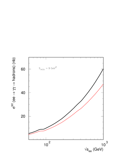
Figure 7: Cross-sections for hadron production due to $\gamma\gamma$ interactions in $e^{+}e^{-}$  reactions.

In Fig. 7, we have shown the cross-section as a function of $\sqrt{s}$ of the $e^{+}e^{-}$ machine. The top curve corresponds to the prediction for $\sigma_{\mbox{$\gamma\gamma$}}$ of the EMM model in the inelastic formulation and the lower curve corresponds to the prediction of the model [24] for the same. It is to be noted that the difference of about factor 2 (say) at $\mbox{$\sqrt{s}$}=700$ GeV, is reduced to about $30\%$ after convolution with the bremsstrahlung spectrum. In this figure we have used $s_{min}=9\ GeV^{2}$, to be consistent with the $p_{\rm tmin}$= 1.5 GeV used in the EMM prediction. If we naively extrapolate the predictions to $s=1\ GeV^{2}$ and thus integrate upto $s_{\rm min}=1\ GeV^{2}$ the hadron production cross-sections go up by about a factor 2. Note also that the reduction in the photon spectrum due to the anti-tagging condition causes a reduction of about 40% at the highest end.

5 Acknowledgments

We have enjoyed discussions with A. Grau and O. Panella and are grateful to M. Kienzle for discussions about the recent data and to A. de Roeck for suggestions concerning the precision issue at Linear Colliders. One of us is indebted to M. Block for discussions on the factorization question for total cross-sections. This work was supported in part through TMR98-0169.

References

- [1] D.Cline, F.Halzen and J. Luthe, Phys. Rev. Lett. 31 (1973) 491.
- [2] M. Drees and R.M. Godbole, Phys. Rev. Lett. 67 (1991) 1189; P. Chen ,T. Barklow and M.E. Peskin, Phys. Rev. D49 (1994) 3209, R.M. Godbole, hep-ph/9807379, Proceedings of the Workshop onQuantum Aspects of Beam Physics, Jan. 5 1998 - Jan. 9 1998, Monterey, U.S.A., 404-416, Ed. P. Chen, World Scientific, 1999.
- [3] For a review, see for example, M. Drees and R.M. Godbole, Journal of Phys. G 21 (1995) 1559.
- [4] A. Corsetti, R.M. Godbole and G. Pancheri, Phys.Lett. B435 (1998) 441.
- [5] OPAL Collaboration. F. Waeckerle, Multiparticle Dynamics 1997, Nucl. Phys. Proc. Suppl. B71, (1999) 381, Eds. G. Capon, V. Khoze, G. Pancheri and A. Sansoni; Stefan Söldner-Rembold, hep-ex/9810011, To appear in the proceedings of the ICHEP’98, Vancouver, July 1998. G. Abbiendi et al.,Eur.Phys.J.C14 (2000) 199.
- [6] L3 Collaboration, Paper 519 submitted to ICHEP’98, Vancouver, July 1998. M. Acciari et al., Phys. Lett. B 408 (1997) 450; L3 Collaboration, A. Csilling, Nucl.Phys.Proc.Suppl. B82 (2000) 239.
- [7] L3 Collaboration, L3 Note 2548, Submitted to the OSAKA Conference.
- [8] L. Durand and H. Pi, Phys. Rev. Lett. 58 (1987) 58. A. Capella, J. Kwiecinsky, J. Tran Thanh, Phys. Rev. Lett. 58 (1987) 2015. M.M. Block, F. Halzen, B. Margolis, Phys. Rev. D 45 (1992) 839.
- [9] A. Capella and J. Tran Thanh Van, Z. Phys. C 23 (1984)168. G. Pancheri and C. Rubbia, Nucl. Phys. A 418 (1984) 117c. T.Gaisser and F.Halzen, Phys. Rev. Lett. 54 (1985) 1754. P. l‘Heureux, B. Margolis and P. Valin, Phys. Rev. D 32 (1985) 1681. G.Pancheri and Y.N.Srivastava, Phys. Lett. B 158 (1986) 402.
- [10] M. Glück, E. Reya and A. Vogt, Zeit. Physik C 67 (1994) 433 . M. Glück, E. Reya and A. Vogt, Phys. Rev. D 46 (1992) 1973.
- [11] D. Treleani and L. Ametller, Int. Jou. Mod. Phys. A 3 (1988) 521
- [12] A. Grau, G. Pancheri and Y.N. Srivastava, Phys.Rev. D60 (1999) 114020.
- [13] J.C. Collins and G.A. Ladinsky, Phys. Rev. D 43 (1991) 2847.
- [14] R.S. Fletcher , T.K. Gaisser and F.Halzen, Phys. Rev. D 45 (1992) 377; erratum Phys. Rev. D 45 (1992) 3279.
- [15] K. Honjo, L. Durand, R. Gandhi, H. Pi and I. Sarcevic, Phys. Rev. D 48 (1993) 1048.
- [16] R.M. Godbole and G. Pancheri, Proceedings of the LUND workshop on photon interactions and photon structure, Aug. 1998, 217-227, Eds. T. Sjostrand and J. Jarsklog, e-print Archive: hep-ph/9903331.
- [17] M. Derrick et al., ZEUS coll., Phys. Lett. B 354 (1995) 163.
- [18] R.M. Godbole, A. Grau and G. Pancheri. Nucl.Phys.Proc.Suppl.B82 (2000), hep-ph/9908220.
- [19] G. Schuler and T. Sjöstrand, Zeit. Physik C 68 (1995) 607; Phys. Lett. B 376 (1996) 193.
- [20] M. Glück, E. Reya and I. Schienbein, Phys.Rev.D60:054019, 1999, Erratum-ibid.D62:019902,2000.
- [21] ZEUS Collaboration, Phys. Lett. B 293 (1992), 465; Zeit. Phys. C 63 (1994) 391.
- [22] H1 Collaboration, Zeit. Phys. C69 (1995) 27.
- [23] J. Breitweg et al., ZEUS coll., DESY-00-071, e-print Archive: hep-ex/0005018.
- [24] M.M. Block, E.M. Gregores, F. Halzen and G. Pancheri, Phys.Rev.D58 (1998) 17503; M.M. Block, E.M. Gregores, F. Halzen and G. Pancheri, Phys.Rev. D60 (1999) 54024.
- [25] C. Bourelly, J. Soffer and T.T. Wu, Mod.Phys.Lett. A15 (2000) 9.
- [26] A. Donnachie and P.V. Landshoff, Phys. Lett.B 296 (1992) 227.
- [27] B. Badelek, M. Krawczyk, J. Kwiecinski and A.M. Stasto. e-Print Archive: hep-ph/0001161.
- [28] E. Gotsman, E. Levin, U. Maor, E. Naftali, Eur.Phys.J. C14 (2000) 511, hep-ph/0001080.
- [29] R. Godbole, A. Grau and G. Pancheri, QCD and Multiparticle Production, page 424. Proceedings of the XXIX International Symposium on Multiparticle Dynamics, Brown U., Aug. 2000. Eds. I. Sarcevic and C-I Tang. World Scientific 2000. e-print Archive: hep-ph/9912395.
- [30] M. Drees and R.M. Godbole, Zeit. Phys. C 59 (1993) 591.
- [31] C.F. v. Weizsäcker, Z. Phys. 88, 612 (1934); E.J. Williams, Phys. Rev. 45 729.
- [32] For a recent discussion, see for example, S. Frixione, M.L. Mangano, P. Nason and G. Ridolfi, Phys. Lett. B319, 339 (1993).
- [33] M. Drees and R.M. Godbole, Phys. Rev. D 50 (1994) 3124.