Moduli Evolution in Heterotic Scenarios

We discuss several aspects of the cosmological evolution of moduli fields in heterotic string/M-theory scenarios. In particular we study the equations of motion of both the dilaton and overall modulus of these theories in the presence of an expanding Universe and under different assumptions. First we analyse the impact of their couplings to matter fields, which turns out to be negligible in the string and M-theory scenarios. Then we examine in detail the possibility of scaling in M-theory, i.e. how the moduli would evolve naturally to their minima instead of rolling past them in the presence of a dominating background. In this case we find interesting and positive results, and we compare them to the analogous situation in the heterotic string.

CERN-TH/2000-302
SUSX-TH/00-014
September 2000

CERN-TH/2000-302

1 Introduction

For a number of years now, our knowledge of the string world has greatly improved with the discovery of M-theory as the origin of all the known perturbative string theories [1]. In particular, the $D=11$ supergravity (SUGRA) limit of this theory (also known as M-theory itself) has been extensively studied and, by now, we have quite a deep understanding of many aspects of it.

However the issue of how to stabilize the moduli in these theories, and the role they play in cosmology, is still an open one. This is because, in order to generate a potential for the moduli, we must rely on non-perturbative physics which is not under our control. Still, a few general results can be obtained, which encourage further investigation. In particular, supersymmetry (SUSY) breaking by gaugino condensation [2] in the $D=4$ effective theory works in a similar way as in the old heterotic string [3]. In fact it is possible to build many scenarios where multiple gaugino condensates contribute to create a scalar potential for the moduli $S$ and $T$ that has minima at the phenomenologically desired values (${\rm Re}\;S,{\rm Re}\;T\sim O(20)$ in $M_{\rm P}$ units) [4]. Also the fact that the gaugino condensates depend exponentially on the gauge kinetic functions ($\sim e^{-\alpha_{a}f_{a}}$, where $a$ labels each condensate, $\alpha_{a}$ are related to the 1-loop beta function coefficients and $f_{a}$ are the gauge kinetic functions), with $4\pi f_{a}=S-\beta_{a}T$, instead of $f_{a}=k_{a}S$ as it was the case in the heterotic string, gives rise to the appearance of flat directions in the scalar potential, opening up the possibility of inflation along those. This was thoroughly studied in Ref. [5].

Despite of these promising results, there is a second issue we want to address in this letter, which is the dynamical evolution of the other moduli, i.e. those which do not have a flat direction and therefore would suffer from a ‘runaway problem’, given the exponential nature of their potential. This problem, first pointed out by Brustein and Steinhardt [6] in the context of the heterotic string, has been studied along the years and several mechanisms have been proposed in order to alleviate it (see Refs [7, 8, 9]). Our goal will be, exploiting the similarity between the heterotic string and M-theory scenarios pointed out above, to examine this mechanism for dynamically stabilizing moduli in the context of heterotic M-theory.

In order to do so, in section 2 we revise the status of the runaway problem in the heterotic string, with particular emphasis on the recently proposed mechanism of Huey et al. [9], and its applicability to string models. In section 3 we discuss the M-theory setup: first we study the existence of scaling solutions in the presence of a dominating background and then we consider the above-mentioned couplings of the moduli to matter. Finally, we conclude in section 4.

2 Scaling solutions revisited

Let us briefly review the issue of scaling solutions in gaugino condensation models. It is by now a standard result in cosmology that scalar fields with an exponential scalar potential have scaling solutions that are global attractors [10, 11, 12]. In these scaling solutions the field will evolve with the same equation of state as the background energy density. As was explained in Ref. [8], the dilaton, $S$, in the heterotic string theory is a perfect example of such scaling behaviour. This scalar particle has an exponential type potential which is steep enough to make the field roll past its minimum. However, if the energy density of the Universe includes some barotropic fluid coupled to the dilaton only gravitationally, this field will reach a constant velocity at late times, and will evolve slowly down the exponential slope. This behaviour, however, can only stabilize the dilaton if it starts its evolution to the left of its minimum.

More recently a new mechanism has been proposed [9] which could help stabilizing moduli with exponential potentials both in their strong and weak coupling regimes. It relies on the existence of couplings of these moduli (generically denoted by $\phi$, with an exponential type potential $V_{0}(\phi)$) to matter fields (which we will call $C$). These can occur either through the kinetic terms (which, following Ref. [9], we parametrise as $f(\phi)\partial_{\mu}C\partial^{\mu}C$) or through the scalar potential ($V_{1}\sim g(\phi)C^{n}$). Assuming the $C$ field to be homogeneous, we define its energy density and pressure to be respectively,

$$\rho_{C} = f\dot{C}^{2}+V_{1}\;\;,$$ (1)

$$p_{C} = f\dot{C}^{2}-V_{1}\;\;.$$ (2)

The equations of motion for $\phi$ and $\rho$ are then given by

$$\ddot{\phi}+3H\dot{\phi}-\frac{\partial p_{C}}{\partial\phi}+\frac{\partial V_{0}}{\partial\phi}=0\;\;,$$ (3)

$$\dot{\rho_{C}}=-\left(3H+\frac{\dot{f}}{2f}\right)(\rho_{C}+p_{C})+\frac{\dot{g}}{2g}(\rho_{C}-p_{C})\;\;,$$ (4)

with $H^{2}=\frac{1}{3}(\dot{\phi}^{2}/2+V_{0}+\rho_{C})$. To be precise, we will consider the case where the $C$ field has coherent oscillations about its minimum. In this case, the energy density and pressure, averaged over one oscillation, will obey the equation of state $p_{C}=w_{C}\rho_{C}$, with $w_{C}=(n-2)/(n+2)$ from the virial theorem. We do this in order to have a simple barotropic fluid as a background. A similar situation could be obtained if we considered instead the field $C$ to be in thermal equilibrium [9].

With these assumptions, the pressure derivative in Eq. (3) becomes

$$\frac{\partial p_{C}(\phi,C,\dot{C})}{\partial\phi}=\left((1+w_{C})\frac{1}{f}\frac{\partial f}{\partial\phi}-(1-w_{C})\frac{1}{g}\frac{\partial g}{\partial\phi}\right)\frac{\rho_{C}}{2}\;\;,$$ (5)

and Eq. (4) can be exactly solved to give

$$\rho_{C}(\phi,a)=\rho_{0}\left(\frac{a}{a_{0}}\right)^{-3(1+w_{C})}\left(\frac{f}{f_{0}}\right)^{-(1+w_{C})/2}\left(\frac{g}{g_{0}}\right)^{(1-w_{C})/2}\;\;,$$ (6)

where $a$ is the scale factor of the Universe and the subscript ₀ denotes initial values of the corresponding functions. Altogether we see that the new term $-\partial p_{C}/\partial\phi$ can be interpreted as a contribution to the total scalar potential of the $\phi$ field. In other words, the coupled system will be equivalent to a single field system with a total potential given by

$$V_{\rm tot}=V_{0}(\phi)+V_{\rm eff}(\phi)\;\;,$$ (7)

with

$$V_{0}(\phi)\sim e^{-\alpha\phi}$$ (8)

and

$$V_{\rm eff}(\phi)=\rho_{C}(\phi)\;\;.$$ (9)

Notice that $\rho_{C}$ is now given by Eq. (6), an explicit function of time (or the scale factor, $a$), as opposed to the $\rho_{C}$ we had before integrating out the $C$ field. They have both the same value of course, but their partial derivatives with respect to $\phi$ will be different. In particular, it is easy to show that

$$\frac{\partial\rho_{C}(\phi,a)}{\partial\phi}=-\frac{\partial p_{C}(\phi,C,\dot{C})}{\partial\phi}\;\;,$$ (10)

the result we have used to obtain Eq. (9). This effective potential is represented in Fig. 1a, where we show the shape of $V_{\rm tot}$ as a function of $\phi$, for several values of $N\equiv\ln(a)$ with $w_{C}=1/3$, for the particular case of $f(\phi)=g(\phi)=1/\phi$ considered in Ref. [9]. Here $V_{0}$ is given by a two condensate model analogous to Eq. (4) of Ref. [9]. We can see that, at earlier times (i.e. for $N$ small), the potential has a growing slope to the right of the minimum, whose position changes with $N$. At late enough times (i.e. for $N$ large) this effective contribution fades away and we recover the original exponential potential $V_{0}(\phi)$. As we see in Fig. 1b, even for initial conditions in the very weak coupling regime (characterised by large values of $\phi$), the field rolls towards its minimum.

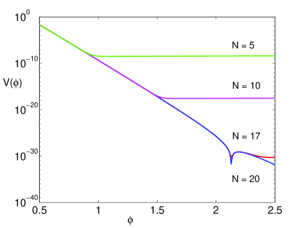
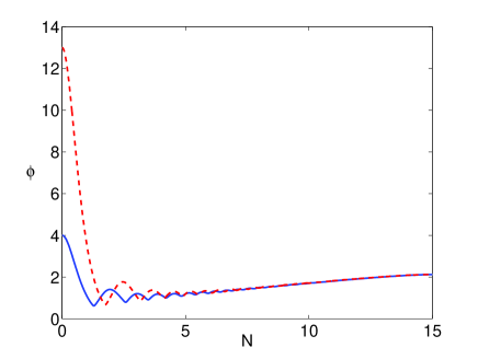
Figure 1:

(a) Plot of the total scalar potential, given by Eq. (7), as a function of the dilaton $\phi$ (in $M_{P}$ units) in a two condensate model with groups ${\rm SU}(6)_{2}\times{\rm SU}(7)_{8}$ and $T_{\rm R}=1.23$ (see footnote 2). The different curves correspond to different times -or number of $e$-folds $N$- in the evolution of the system. (b) Evolution of the dilaton ($\phi$), as in Eq. (11), as a function of $N\equiv\ln(a)$, for the same example as in Fig. 1a and initial conditions given by $\phi_{0}=13$ (dashed), $\phi_{0}=4$ (solid).

Despite of how promising this mechanism looks as a way of stabilizing moduli, it is very sensitive to the particular forms of the functions $f$ and $g$ (recall $f=g=1/\phi$ in the above example). Therefore it is a natural step to proceed with the study of string inspired models and, in particular, we shall devote some time to consider the dilaton of the heterotic string and its couplings.

The first thing one must take into account is that, in the context of the heterotic string, the dilaton $S$ is not a canonically normalised field, i.e. its kinetic term is given by $K_{S\bar{S}}\partial_{\mu}S\,\partial^{\mu}{\bar{S}}$, with $K_{S\bar{S}}=\partial^{2}K/\partial S\partial\bar{S}$ and the tree-level Kähler potential given by $K=-\ln(S+\bar{S})$. Therefore its equation of motion reads

$$\ddot{S}+3H\dot{S}+\frac{K_{S\bar{S}\bar{S}}}{K_{S\bar{S}}}\dot{S}^{2}-\frac{1}{K_{S\bar{S}}}\frac{\partial p_{C}}{\partial{\bar{S}}}+\frac{1}{K_{S\bar{S}}}\frac{\partial V}{\partial{\bar{S}}}=0\;\;,$$ (11)

where $K_{S\bar{S}\bar{S}}=\partial K_{S\bar{S}}/\partial\bar{S}$ and $H^{2}=\frac{1}{3}(K_{S\bar{S}}\dot{S}^{2}+K_{C\bar{C}}\dot{C}^{2}+V(S,C))$. It must be said, however, that the term proportional to $\dot{S}^{2}$ is negligible in the region of values of $S$ studied here, and therefore this equation is very similar to the simpler Eq. (3) described previously. The couplings to matter, contained in $\partial p_{C}/\partial S$, are determined by the structure of the N=1 SUGRA Lagrangian that describes this string-inspired model. The kinetic term for $C$ reads [13]

$$K_{C\bar{C}}\partial_{\mu}C\partial^{\mu}\bar{C}=\frac{3}{2T_{\rm R}}\left(1+\frac{\epsilon}{6S_{\rm R}}\right)\partial_{\mu}C\partial^{\mu}\bar{C}\;\;,$$ (12)

where $\epsilon=\delta_{GS}/4\pi^{2}$ is the so-called Green–Schwarz coefficient, which is generally small, and $S_{\rm R}\equiv{\rm Re}S$, $T_{\rm R}\equiv{\rm Re}T$. Therefore in the parametrisation introduced before Eq. (1), $f(S_{\rm R})$ is given by

$$f(S_{\rm R})=\frac{3}{2T_{\rm R}}\left(1+\frac{\epsilon}{6S_{\rm R}}\right)\;.$$ (13)

Finally, the form of the scalar potential is given by

$$V=e^{K}\left\{\sum_{i,j}(W_{i}+K_{i}W){(K_{i}^{j})}^{-1}(\bar{W}^{j}+K^{j}\bar{W})-3|W|^{2}\right\}\;\;,$$ (14)

where sub(super)scripts denote derivatives of $W$ and $K$ with respect to $S$ ($\bar{S}$) and $C$ ($\bar{C}$), and $W\sim\sum_{a}e^{-\alpha_{a}S}+C^{3}$ is the superpotential coming from multiple gaugino condensation. The couplings between the two fields $S$ and $C$ arise from the term $e^{K}|K_{C}W+W_{C}|^{2}/K_{C\bar{C}}$. For $C$ small, $W_{C}\sim C^{2}$ will dominate and we can identify

$$g(S_{\rm R})=e^{K}/K_{C\bar{C}}=\frac{1}{24T_{\rm R}^{2}S_{\rm R}}\;.$$ (15)

Therefore this coupling is of the form $1/S_{\rm R}$.

We can now solve Eq. (11), and the result is that $S_{\rm R}$ has the same runaway behaviour that it would have had in the absence of the couplings to matter. Let us briefly sketch why the mechanism of Ref. [9] does not work here: consider the general form for the couplings $f=a+b/S_{\rm R}$, $g=c+d/S_{\rm R}$, with $a$, $b$, $c$, $d$ real and positive. A slope to the right of the minimum, such as those in Fig. 1a, will appear if, in Eq. (11), we require $-\partial p_{C}/\partial S>0$ to balance $\partial V/\partial S$ which is invariably negative (recall that $V\sim e^{-\alpha S}$). From Eq. (5) is it easy to translate this condition, for positive $w_{C}$, into either of these two

$$i)\;ad(1-w_{C})-bc(1+w_{C}) \leq 0$$

$$ii)\;ad(1-w_{C})-bc(1+w_{C}) > 0\;\;{\rm and}\;\;S_{\rm R}<\frac{2bdw_{C}}{ad(1-w_{C})-bc(1+w_{C})}\;.$$

In Ref. [9], indeed $w_{C}=1/3$ is positive and $f$ and $g$ are such that $a=c=0$, that is this choice fulfils condition i) and their $\phi$ field is always trapped at the minimum. In the heterotic string, however, $c=0$ and $a\neq 0$, so we are in case ii), which implies that the dilaton will be trapped only for initial conditions $S_{\rm R}\stackrel{{\scriptstyle<}}{{{}_{\sim}}}b/a=\epsilon/6\ll 1$, for any values of $w_{C}\neq 1$. This corresponds to the strong coupling regime and covers a very small fraction of the parameter space. For completeness we can also consider the case in which $-1\leq w_{C}\leq 0$, and now we will have only one condition for $-\partial p_{C}/\partial S>0$, which is

$$ad(1-w_{C})-bc(1+w_{C})<0\;\;{\rm and}\;\;S_{\rm R}>\frac{2bdw_{C}}{ad(1-w_{C})-bc(1+w_{C})}\;.$$ (17)

It is easy to see that, again, for the heterotic string where $c=0$, this condition can never be fulfilled.

Therefore to end this section we should conclude that, concerning the probability of stabilizing the moduli in the Early Universe, the estimates of Horne and Moore [7] still represent the most optimistic situation. They argued that the motion of the moduli follows a chaotic trajectory and, out of the finite volume of possible initial conditions, 12-14% of it corresponds to cases where the dilaton will end up at its minimum. However, in Ref. [14] it was pointed out how, in their scenario, the inhomogeneous modes would soon come to dominate the energy density of moduli fields. Finally, if we consider the presence of a dominating background, then the estimates of Ref. [8] remain unaltered in the presence of above-mentioned couplings to matter fields.

3 Dynamics of the moduli in M-theory

In this section we will try to apply the same ideas, namely the evolution of moduli fields in the presence of some background matter, to study the evolution of the real parts of the $S$ and $T$ moduli in heterotic M-theory. From a phenomenological point of view, one of the main differences between the two models is that the gauge kinetic functions in the hidden wall, $f_{a}$ (whose VEV determine the gauge coupling constants) are now a linear combination of the string dilaton and modulus fields, i.e $f_{a}=(S-\beta_{a}T)/(4\pi)$ where $\beta_{a}$ are constants that depend on the details of the model and are usually of order one [15] (in particular, in all the examples shown in this paper we have fixed $\beta_{a}=\beta=1/2$). Assuming once again that gaugino condensation is the source of SUSY breaking, the scalar potential will have an exponential like profile, as in the string case, along the direction defined by $\Phi_{-}\equiv S-\beta T$. Along its orthogonal direction, $\Phi_{+}\equiv\beta S+T$, the potential will be almost flat, the only dependence upon this variable coming from the Kähler potential $K$. We will consider potentials where a minimum is generated along the $\Phi_{-}$ direction with two gaugino condensates. This defines a ‘valley’ in the $\Phi_{+}$ direction with an inverse power law profile, and the global minimum is obtained with a third condensate, or a non-perturbative correction to the Kähler potential [4, 5].

Let us start with the simplest case, when the $S$ and $T$ fields have no direct coupling to the background fluid. As we have just said we have essentially two major directions in our scalar potential, an exponential slope for the $\Phi_{-}$ field and an inverse power-law for the $\Phi_{+}$ field. In the exponential part of the potential we expect the field $\Phi_{-}$ to dominate the evolution, behaving in a similar way to the dilaton in the heterotic string case [8]. However, in the valley defined by $\Phi_{-}=\Phi_{-}^{\rm min}$, we expect the evolution to be driven by the $\Phi_{+}$ field along the valley. Therefore the stabilization of the fields will rely on a two-step process, first the evolution into the valley, and then the stabilization along the valley to the minimum (see Fig. 2).

We will analyse the behaviour of the fields in this model using a numerical simulation with a specific example. The equations of motion of the two fields, with no direct couplings to the background, is given by

$$\ddot{S}+3H\dot{S}+\frac{K_{S\bar{S}\bar{S}}}{K_{S\bar{S}}}\dot{S}^{2}+\frac{1}{K_{S\bar{S}}}\frac{\partial V}{\partial{\bar{S}}} = 0\;\;$$ (18)

$$\ddot{T}+3H\dot{T}+\frac{K_{T\bar{T}\bar{T}}}{K_{T\bar{T}}}\dot{T}^{2}+\frac{1}{K_{T\bar{T}}}\frac{\partial V}{\partial{\bar{T}}} = 0\;\;,$$ (19)

with the Hubble constant now being given by

$$H^{2}=\frac{1}{3}(K_{S\bar{S}}\dot{S}\dot{\bar{S}}+K_{T\bar{T}}\dot{T}\dot{\bar{T}}+V+\rho_{\rm B})\;\;,$$ (20)

where $\rho_{\rm B}$ is the background energy density. We evolve both fields simultaneously, since the flat directions in the scalar potential do not coincide with the ones in the Kähler potential. As detailed in Ref. [5], the scalar potential is explicitly given by

$$V=e^{K}\left\{\frac{1}{K_{S\bar{S}}}|W_{S}+K_{S}W|^{2}+\frac{1}{K_{T\bar{T}}}|W_{T}+K_{T}W|^{2}-3|W|^{2}\right\}\;\;,$$ (21)

where $W$, the superpotential for multiple gaugino condensation, reads as

$$W=\sum_{a}C_{a}e^{-\alpha_{a}\Phi_{-}}\;,$$ (22)

with $C_{a}$ and $\alpha_{a}$ being constants related to the one-loop beta-function coefficients of the corresponding condensing groups. We will consider for the numerical examples the case of two condensates, ${\rm SU}(3)\times{\rm SU}(4)$, with 8 pairs of matter fields transforming as $(4,\bar{4})$. The Kähler potential is given by

$$K(S_{\rm R},T_{\rm R})=-\log(S+\bar{S})-3\log(T+\bar{T})+K_{\rm np}(S_{\rm R})\;\;,$$ (23)

where the first two terms are the tree level result and $K_{\rm np}$ accounts for non-perturbative corrections. We will use for the numerical examples the ansatz for $K_{\rm np}$ introduced in Ref. [17],

$$K_{\rm np}=\frac{D}{B\sqrt{S_{\rm R}}}\log\left(1+e^{-B(\sqrt{S_{\rm R}}-\sqrt{S_{0}})}\right)\;\;$$ (24)

where we fix $S_{0}=19$, and for each particular value of $B$ we choose $D$ so that the cosmological constant is equal to zero.

Let us then start analysing the evolution of the fields outside the valley in the scalar potential. In Fig. 3 we show the numerical evolution of the fields’ equation of state, $w_{\Phi}$, as a function of $\Phi_{-}$ before the fields reach the valley at $\Phi_{-}^{\rm min}=11.07$. A set of different initial conditions and different types of background fluid were considered.

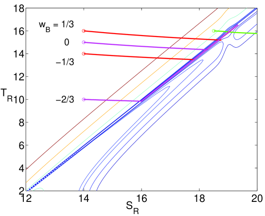
Figure 2:

Contour plot of the scalar potential $V$ in terms of $S_{\rm R}$, $T_{\rm R}$. The thick lines represent the trajectories of the fields in the presence of the corresponding backgrounds, in particular the upper right line corresponds to no background present. The parameters used for $K_{\rm np}$ are $B=120$ and $D=0.13$. One can see that when a background fluid is present, the range of initial conditions allowing stabilization is highly improved.

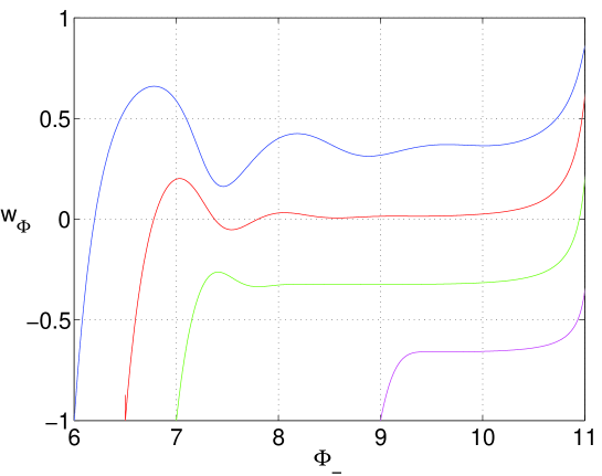
Figure 3:

Equation of state of the system of fields $\Phi_{-}$, $\Phi_{+}$ as a function of $\Phi_{-}$ before reaching the minimum at $\Phi_{-}^{\rm min}\approx 11.07$. From top to bottom the different curves correspond to the following choice of background ($w_{B}$): 1/3, 0, -1/3, -2/3.

It is easy to see from this plot that the behaviour of the fields outside the valley is very similar to the case of the dilaton in the heterotic string case. That is, they will quickly reach a scaling solution in which their energy density scales with the background with roughly the same equation of state (i.e. $w_{\Phi}\sim w_{B}\equiv p_{B}/\rho_{B}$). As in the string case, this will be enough to slow down the evolution of the fields and allow them to settle in the valley for a wide range of initial conditions. However, note in Fig. 2 that the evolution of the fields is not orthogonal to the direction of the valley. In other words, $\Phi_{-}$ and $\Phi_{+}$ scale simultaneously. The direction of the evolution is determined from the scalar potential gradient and the Kähler potentials of the two fields, and it is not possible to estimate it analytically.

The main differences with the heterotic string case arise once the fields have settled in the valley. In order to be stabilized, they still have to evolve inside the valley towards the minimum. The valley corresponds approximately to a constant $\Phi_{-}$, which we denote as $\Phi^{\rm min}_{-}$, so that the evolution at this stage will be dominated by the $\Phi_{+}$ field. The effective scalar potential for the $\Phi_{+}$ field is power-law like. To be precise, the dominating term is the $e^{K}$ factor in Eq. (21), that is

$$V\approx\frac{V_{0}}{(\beta\Phi_{+}+\Phi_{-}^{\rm min})(\Phi_{+}-\beta\Phi_{-}^{\rm min})^{3}}\;\;,$$ (25)

where $V_{0}$ is a constant that can be estimated analytically (exactly for the D=0 case) and $\Phi_{-}^{\rm min}$ is understood to be held constant. In this approximation, where $\Phi_{-}$ is constant, one can also write an effective kinetic term for the $\Phi_{+}$ field given in terms of the kinetic terms for the $S$ and $T$ fields. Namely, since $S=(\beta\Phi_{+}+\Phi_{-})/(1+\beta^{2})$ and $T=(\Phi_{+}-\beta\Phi_{-})/(1+\beta^{2})$, we have that

$$K_{S\bar{S}}\dot{S}^{2}+K_{T\bar{T}}\dot{T}^{2}\approx\frac{\beta^{2}K_{S\bar{S}}+K_{T\bar{T}}}{(1+\beta^{2})^{2}}\;{\dot{\Phi}_{+}}^{2}\;\;.$$ (26)

The final result is a field which has a power-law type potential and a kinetic term that is inversely proportional to $\Phi_{+}^{2}$. If we transform it into a real field, $\sigma$, with canonical kinetic terms, $\frac{1}{2}\dot{\sigma}^{2}$, it is easy to check that $\sigma=\sqrt{2}\;\log{\Phi_{+}}$ and therefore its effective scalar potential will be an exponential. Hence, we expect the behaviour at late times to be the usual scaling solution associated with exponential potentials. To be more precise, for large values of the field the effective potential, Eq. (25), goes as $1/\Phi_{+}^{4}$, and therefore the effective scalar potential for $\sigma$ is $V(\sigma)=e^{-2\sqrt{2}\sigma}$. Without a minimum, that is for $K_{\rm np}=0$, this is exactly the scaling solution one obtains numerically for late times.

This is a nice result in itself, showing that the fields tend to join scaling solutions (albeit ones of different type) when in the presence of a background, both in the valley and outside it. However, the time the fields take to reach the scaling solution in the valley is considerably longer. This means that they will usually reach the minimum of the potential before acquiring a scaling behaviour. This in itself does not stop the fields from being trapped at the minimum, since the background is already slowing them down considerably, but it does mean that an analytical approach is much more difficult, since the field reaches the minimum at an intermediate regime, between prescaling and scaling.

We can have an idea of the range of initial conditions that stabilize the fields by looking at Table 1. First of all, if the value of $\rho_{B}^{0}$ is too small, the fields will begin to evolve as if there was no background (that is, they will not stay in the minimum unless they start really close to it). Once the background becomes important, the actual value of $\rho_{B}^{0}$ does not really affect the evolution, since the fields will just stay frozen until the energy densities of the fields and background become comparable. Therefore we chose to fix $\rho_{B}^{0}=10^{20}$ in the examples given in Table 1. The value of $w_{B}$, on the other hand, affects drastically the results. The lower it is, the easier it is for the fields to be stabilized. This is not too surprising, since a smaller $w_{B}$ corresponds to a universe where the potential terms dominate over the kinetic terms (and recall that the fields will mimic the background once they reach their scaling solutions). Moreover, different values of the $(B,D)$ parameters in the non-perturbative Kähler will give slightly different answers. In short, the smaller the $B$ parameter, the less fine tuned is the minimum in the scalar potential, and the easier it is to stabilize the fields. Finally, one can check that the further the fields are from the minimum when they hit the valley, the more difficult the stabilization becomes. The full evolution for specific examples where stabilization is achieved can be seen in Fig. 2.

$K_{\rm np}$ $(B,D)$	$T_{\rm R}^{0}$	$w_{B}$	Stability
(120, 0.13)	16	1/3	$\surd$
(120, 0.13)	14	0	$\times$
(120, 0.13)	14	-1/3	$\surd$
(120, 0.13)	10	-1/3	$\times$
(120, 0.13)	10	-2/3	$\surd$
(120, 0.13)	6	-2/3	$\times$
(50, 0.33)	6	-2/3	$\surd$
(50, 0.33)	6	-1/3	$\times$
(10, 2.18)	6	-1/3	$\surd$
(10, 2.18)	6	0	$\times$

Table 1: Examples of points in parameter space for which the fields are -or not- stabilized at the minimum. In all of them $\rho_{B}^{0}=10^{20}$ and $S_{\rm R}^{0}=14$.

Let us finally turn to the case where the dilaton and modulus fields have direct couplings to the background fields. As for the string case considered in Section 2, we will again model the background as a scalar field $C$ with a coupling $f(S_{\rm R},T_{\rm R})$ in the kinetic terms, and $g(S_{\rm R},T_{\rm R})$ in the scalar potential. Its energy density and pressure is again given by Eqs (1,2) and the dilaton and modulus equations of motion by Eq. (18) and Eq. (19) respectively. The couplings are now functions of both fields [15], namely

$$f(S_{\rm R},T_{\rm R}) = \frac{3}{2T_{\rm R}}+\frac{\beta}{2S_{\rm R}}\;\;,$$ (27)

$$g(S_{\rm R},T_{\rm R}) = \frac{1}{4T_{\rm R}^{2}(3S_{\rm R}+\beta T_{\rm R})}\;\;.$$ (28)

The situation here is similar to the heterotic string case if slightly more involved. Again, $\partial V/\partial S$ is always negative (except near the valley where the condensates cancel each other), and the $S$ field tends to go to infinity. If the interaction term in Eq. (11) is to cancel this natural tendency, then we require $\partial p_{C}/\partial S<0$. It is easy to check that, for positive $S$ and $T$, this is equivalent to $S<2\beta/3T$. This only happens for $S$ smaller than its minimum value, so if the initial conditions are larger than this, the field will always run away to infinity. For the $T$ field, however, things do change. The derivative term $\partial V/\partial T$ is always positive (again, except near the valley), and therefore the field will tend to go to zero (it will never become negative since its kinetic term diverges at zero). It is possible to check that $\partial p_{C}/\partial T$ has the same sign as $p_{C}$ and therefore, for positive background pressure, the coupling term balances the potential term in the equation of motion for $T$. Indeed, we have checked numerically that the $T$ field will tend to go to a non-zero constant in the presence of these coupling terms. This can also be understood analytically if one looks for the asymptotic solutions in this regime.

Finally let us add that this analysis was performed in the absence of non-perturbative corrections to the Kähler potential, $K_{\rm np}(S_{\rm R})$ (notice the form of Eq. (28)). In the presence of such corrections, that would only affect the behaviour of the $S$ field, we would have to replace Eq. (28) by $e^{K_{\rm np}}g(S_{\rm R},T_{\rm R})$, and its derivative with respect to $S_{\rm R}$ would be now $e^{K_{\rm np}}(\partial g/\partial S_{\rm R}+g\partial K_{\rm np}/\partial S_{\rm R})$. Given that $\partial K_{\rm np}/\partial S_{\rm R}$ is also negative, this would not alter the conclusions we just reached about the evolution of $S$.

In short, adding the interaction terms only improves the situation for the $T$ field. In practice, this means that the fields still have to start to the left of the valley in the scalar potential if they are to become trapped at the minimum. We did not find any improvement in the allowed regions of parameter space presented in Table 1 when we included couplings with the matter fields.

4 Conclusions

In this letter we have addressed the dynamical evolution of moduli fields in several string/M-theory scenarios. In all of them the dynamics are provided by assuming gaugino condensation in the hidden sector of the theory as the source of SUSY breaking and, therefore, of a non flat potential for these fields. Following our previous work on the existence of scaling solutions for the dilaton evolution in the heterotic string, which provided a solution to the so-call ‘runaway problem’ pointed out by Brustein and Steinhardt, we investigated here the impact of a recent proposal to also stabilize moduli of considering the couplings of moduli to matter fields. After a thorough study of the issue in the context of the heterotic string we concluded that these couplings do not seem to affect stabilization for realistic string settings.

Next we considered M-theory scenarios, where there is also a runaway problem associated, in this case, to the combination of dilaton and modulus, $\Phi_{-}$, which has an exponential-type potential analogous to that of the dilaton in the heterotic string. Here we study the evolution equations for both $\Phi_{+}$ and $\Phi_{-}$ in the presence of a dominating background, in order to see whether we can also reach a scaling regime that will make the fields settle at their minima instead of rolling past them. It turns out that such a regime, i.e. scaling, is achieved but at late stages of the moduli evolution, with the result that these fields are not stabilized while scaling, but in an intermediate regime. This makes it extremely difficult to perform an analytic study of the problem but, nevertheless, we have been able to determine a wide region of the parameter space (essentially defined by the initial positions of the fields, the type of background and the characteristics of the non-perturbative Kähler potential) for which the stabilization is successful. Finally, we considered the couplings of moduli to matter fields, and we concluded that the situation is the same as in the heterotic string case, i.e. these couplings do not contribute at all to improve the stabilization problem of the moduli.

References

-
[1]
P. Hořava, E. Witten, Nucl. Phys. B460 (1996) 506 and B475 (1996) 94;
E. Witten, Nucl. Phys. B471 (1996) 135. -
[2]
P. Hořava, Phys. Rev. D54 (1996) 7561;
H.P. Nilles, M. Olechowski, M. Yamaguchi, Phys. Lett. B415 (1997) 24 and Nucl. Phys. B530 (1998) 43;
Z. Lalak, S. Thomas, Nucl. Phys. B515 (1998) 55 and Nucl. Phys. B575 (2000) 151;
A. Lukas, B.A. Ovrut, D. Waldram, Phys. Rev. D57 (1998) 7529 and JHEP 04 (1999) 009. -
[3]
J.P. Derendinger, L.E. Ibáñez, H.P. Nilles, Phys. Lett. B155 (1985) 65;
M. Dine, R. Rohm, N. Seiberg, E. Witten, Phys. Lett. B156 (1985) 55;
N.V. Krasnikov, Phys. Lett. B193 (1987) 37. - [4] K. Choi, H.B. Kim, H.D. Kim, Mod. Phys. Lett. A14 (1999) 125.
- [5] T. Barreiro, B. de Carlos, JHEP 03 (2000) 020.
- [6] R. Brustein, P.J. Steinhardt, Phys. Lett. B302 (1993) 196.
- [7] J.H. Horne, G. Moore, Nucl. Phys. B432 (1994) 109.
- [8] T. Barreiro, B. de Carlos, E.J. Copeland, Phys. Rev. D58 (1998) 083513.
- [9] G. Huey, P.J. Steinhardt, B.A. Ovrut, D. Waldram, Phys. Lett. B476 (2000) 379.
- [10] C. Wetterich, Nucl. Phys. B302 (1988) 668.
- [11] P.G. Ferreira, M. Joyce, Phys. Rev. Lett. 79 (1997) 4740.
- [12] E.J. Copeland, A. Liddle, D. Wands, Phys. Rev. D57 (1998) 4686.
- [13] D. Lüst, C. Muñoz, Phys. Lett. B279 (1992) 272.
- [14] T. Banks, M. Berkooz, S.H. Shenker, P.J. Steinhardt, Phys. Rev. D52 (1995) 3548.
-
[15]
K. Choi, Phys. Rev. D56 (1997) 6588;
H.P. Nilles, S. Stieberger, Nucl. Phys. B499 (1997) 3;
A. Lukas, B.A. Ovrut, D. Waldram, Nucl. Phys. B532 (1998) 43. -
[16]
T.J. Li, J.L. López, D.V. Nanopoulos, Phys. Rev. D56 (1997) 2602;
E. Dudas, C. Grojean, Nucl. Phys. B507 (1997) 553;
K. Choi, H.B. Kim, C. Muñoz, Phys. Rev. D57 (1998) 7521. - [17] T. Barreiro, B. de Carlos, E.J. Copeland, Phys. Rev. D57 (1998) 7354.