When can long-range charge fluctuations
serve as a QGP signal?

Abstract

We critically discuss recent suggestion to use long-range modes of charge (electric or baryon) fluctuations as a signal for the presence of Quark-Gluon Plasma at the early stages of a heavy ion collision. We evaluate the rate of diffusion in rapidity for different secondaries, and argue that for conditions of the SPS experiments, it is strong enough to relax the magnitude of those fluctuations almost to its equilibrium values, given by hadronic “resonance gas”. We evaluate the detector acceptance needed to measure such “primordial” long-range fluctuations at RHIC conditions. We conclude with an application of the charge fluctuation analysis to the search for the QCD critical point.

]

I Introduction

During the last few years significant attention has been attracted to the issue of event-by-event fluctuations in high energy heavy ion collisions. The original goal of such studies formulated in [1, 2] has been focused on equilibrium thermodynamical fluctuations at freeze-out. It was argued that long and intense final state interaction of secondaries makes heavy ion collision very different from hadronic collisions, in which dynamical fluctuations of quantum origin produce quite different “intermittent” behavior. Experimental data, such as obtained by NA49 collaboration [3], have indeed revealed only very small Gaussian fluctuations of different quantities incompatible with earlier predictions of large non-equilibrium fluctuations, e.g. due to bubble formation during the phase transition. As discussed in [4, 5, 6] in detail, extensive quantities like the total multiplicity, $N$, obtain contributions from final state interaction of secondaries due to resonances, and initial state fluctuations related to the number of participant/spectator nucleons. Furthermore, experimentally, for central collisions $\langle(\Delta N)^{2}\rangle/\langle N\rangle\approx 2$, and both effects share about equally the responsibility for moving this number away from the Poissonian value $\langle(\Delta N)^{2}\rangle/\langle N\rangle=1$. As emphasized in [4, 7], the intensive quantities, such as mean $p_{T}$, particles ratios etc. are determined entirely by the final state effects, and are well represented by the resonance gas.

Other goals of the event-by-event fluctuation analysis have also been discussed. In particular, one of us[8], using the analogy between Big Bang phenomena and the “Little Bang” in heavy ion collisions, suggested to look for primordial “frozen QGP oscillations”, as it is done for anisotropic components of microwave background in the Universe. The idea was inspired by an observation that large-amplitude oscillations can be excited due to instabilities of parton counter-flows at the initial stage [9]. On the other hand, two simultaneous papers, by Asakawa, Heinz and Muller[10] and Jeon and Koch[11] suggested a different set of primordial signals: equilibrium charge fluctuations in QGP, which happen to be factor 2-3 smaller than in the hadron gas.

The idea [10, 11] is based on the well known phenomenon of kinetic slowdown of fluctuation relaxation, provided sufficiently long-range harmonics of a conserved charge density are considered. If the relaxation time happens to be shorter than the lifetime of hadronic stage of the collisions, the authors argue, the values of such fluctuations should deviate from their equilibrium (resonance gas) values towards their earlier, primordial values, typical for QGP.

Although this idea should work for parametrically long-range effects, whether a number of necessary conditions can indeed be fulfilled in realistic heavy ion collisions depends on the answers to the following questions: (i) How fast is the relaxation due to final-state re-scattering in hadronic gas? (ii) How large the detector acceptance should really be, in order to counter the relaxation? (iii) Is there a window of parameters, forbidding resonance gas relaxation but allowing for it at the QGP stage? (iv) If not, what fluctuations should follow from non-equilibrium parton kinetics, at very early pre-QGP stages of the collisions?

In this paper we attempt to answer the first two of those questions.

II Relaxation of the long-range fluctuations

A The setting

In this section we develop analytical description of the time evolution of fluctuations due to rescattering of charged particles in the hadronic gas at the late stages of the heavy ion collision. The following physical picture underlines our approach.

We consider distributions in rapidity space of a conserved net charge (e.g., electric or baryon). We start our description from the beginning of the hadronic phase. In each event this phase “inherits” a certain distribution in rapidity space of the charge from the primordial quark-gluon plasma phase. In the spirit of the statistical approach, we do not consider a specific charge distribution, but an ensemble of distributions corresponding to a set of events. This ensemble of charge distributions is characterized by the mean and the magnitude of fluctuations. The initial magnitude of those fluctuations is the input of our calculation.

The fluctuations of different length, or range, in rapidity space (i.e., different harmonics of the charge distribution) relax on different time scales. The fact that the net charge is conserved is crucial here. Because the relaxation can only proceed via diffusion of the charge, the longer range fluctuations relax slower. The relaxation time grows as a square of the range. Our goal is to provide a quantitative description of this process.

In particular, we shall derive the equation which solves the following problem: Given a certain detector rapidity acceptance window, and given the initial magnitude of the charge fluctuations, to find the time evolution of that magnitude. From the fact that longer range charge fluctuations relax slower, it is evident that fluctuations of total charge in a wider rapidity window relax slower. Using typical numbers for the life-time of the hadronic phase and rescattering properties of the hadronic gas we shall determine how wide the rapidity window must be chosen in order to preserve, to a sufficient extent, the primordial (small) fluctuation magnitude.

B Diffusion in rapidity space

We introduce the density of a conserved net charge $Q$ per unit rapidity, $n(y,\tau)$, as a function of time $\tau$ in a given event. The objects we are really interested in are the fluctuations of the density,

$$f(y,\tau)=n(y,\tau)-n_{0},$$ (1)

In the Bjorken boost invariant scenario $n_{0}$ is proportional to the total charge in the central region, $n_{0}=Q_{\rm total}/y_{\rm total}$, which is a constant within each event.

We begin by considering evolution of $f$ in a given event. The event-by-event fluctuations will be the subject of subsection II D. There we shall also address fluctuations of the total charge ($Q$, or $n_{0}$), which we ignore for now. Since $f$ is a density of a conserved quantity it should obey a diffusion equation in rapidity space:

$$\partial_{\tau}f=\gamma\,\partial^{2}_{y}f,$$ (2)

where $\gamma=\gamma(\tau)$ is the diffusion coefficient. This diffusion equation (2) applies, provided the following conditions are satisfied:
(i) We must assume that fluctuations are sufficiently small, to justify linear approximation in (2). This is reasonable if the number of particles carrying the charge is large, which is fulfilled in sufficiently central heavy ion collisions at the SPS and higher energies.
(ii) We must assume separation of scales — the minimal interval of rapidity we can consider must be much larger than the mean rapidity change of a charged particle in a collision, $\delta y_{\rm coll}$. In other words, $f$ must be averaged over sufficiently wide interval $\Delta y$. As we shall see later, the typical $\delta y_{\rm coll}$ for the electrical charge is of order 0.8, while for the baryon charge it is 0.2. Even in such a large acceptance detector as STAR at RHIC, the coverage does not exceed few units of rapidity. However, we can still consider a somewhat idealized limit of rapidity windows much wider than $\delta y_{\rm coll}$. This can certainly be reasonable for the diffusion of the baryon charge. Moreover, for the ideas we are evaluating to work, this limit is a necessary condition [10, 11]. Indeed, if the rapidity window is not large compared to $\delta y_{\rm coll}$, the fluctuations will relax by ballistic transport of the charge on the time scale of the mean free time $\tau_{\rm free}$ towards their thermodynamic values, too fast for those ideas to work.

It will not be essential for the analysis of this section how the coefficient $\gamma(\tau)$ is calculated. It may be (ideally) determined from first principles of QCD. In the late hadronic stage of the collision, which is our concern in this paper, one can also use a simple formula to estimate $\gamma$. Since, on the microscopic level, $\gamma$ is due to particle collisions:

$$\gamma={(\delta y_{\rm coll})^{2}\over 2\tau_{\rm free}}.$$ (3)

Since we shall be using Eq.(3) in Section III to estimate $\gamma$ (or, rather, its time integral, see below), we shall discuss it here. It is clear that in the collisionless limit, $\tau_{\rm free}\to\infty$, the diffision in rapidity is absent, which is in trivial agreement with Eq.(3). It is instructive to consider also the limit of $\tau_{\rm free}\to 0$ — the ideal hydrodynamic limit. In this limit diffusion is also frozen — particles have no time to propagate. Eq. (3) can still be applied, but one must realize that, effectively, $\delta y_{\rm coll}$ also vanishes in this limit. The reason is that successive rapidity shifts (each of order unity) are not independent but strongly anticorrelated. This happens because a colliding particle has no time to move out of the region of particles of its initial rapidity, and is more likely to scatter back in than further out. This is also related to the fact that space-time rapidity $(1/2)\ln[(t+z)/(t-z)]$ and momentum rapidity can differ significantly in this limit.

In this paper we need to describe late not-so-dense hadronic stage of the collision with $\tau_{\rm free}$ only few times smaller than evolution time, and we shall apply eq.(3) without worrying about complications of the ideal hydro limit. One can also use cascade codes to estimate $\gamma$, or just the diffusion length squared $2\int\gamma d\tau$, directly, with possible anticorrelations already included, bypassing evaluation of $\delta y_{\rm coll}$.

C Langevin equation

Equation (2) describes relaxation of the density $n$ to its equilibrium value. It implies that we average over time scales longer compared to the characteristic time of fluctuation of $f$. If, however, we are interested in fluctuations of $n$ around its equilibrium value, equation (2) is not enough. We must add a noise term:

$${\partial_{\tau}f}=\gamma\,\partial^{2}_{y}f+\xi(y,\tau).$$ (4)

The characteristic autocorrelation time of the noise is of the same order as the time scale of the variation of $f$. This time is very short since the rapidity windows we consider contain many particles: $f$ changes each time any of the particles collides.

The rapidity correlation of the noise can be determined by requiring that equilibrium fluctuations of $f$ are given by thermodynamics. Thus, they are Gaussian with the probability distribution

$$P_{\rm therm}[f]\sim\exp\left\{-\frac{1}{2}\int dydy^{\prime}\ {f(y)f(y^{\prime})\over 2\,\chi(y-y^{\prime})}\right\},$$ (5)

where $\chi$ is the equilibrium density-density correlation function in rapidity, which we need not know explicitly at this point, and we used boost invariance of Bjorken scenario. In other words:

$$\langle f(y)f(y^{\prime})\rangle=\chi(y-y^{\prime}),$$ (6)

where the average is over time. Writing the functional Fokker-Plank equation for the probability density $P[f]$ following from the Langevin equation (4) we find that (5) is a stationary solution when the noise $\xi$ is Gaussian and obeys:

$$\langle\xi(y,\tau)\xi(y^{\prime},\tau^{\prime})\rangle=-2\gamma\,\partial^{2}_{y}\chi(y-y^{\prime})\,\delta(\tau-\tau^{\prime}).$$ (7)

D Fokker-Plank equation

Before we proceed to solving the Langevin equation (4), we should relate the time average in (6) to the event-by-event average. They are the same by ergodicity. However, one should also keep in mind that changes in initial conditions will change the equilibrium value $n_{0}$. Such initial state fluctuations, as discussed in the introduction, can contribute significantly to the observed event-by-event fluctuations of the extensive quantities, such as the total charge $Q$. Such fluctuations are statistically independent from the thermodynamic fluctuations we consider and can be calculated separately and added in quadratures, as is done in [6]. In contrast, for intensive quantities, such as, for example, the ratio of positively to negatively charged particles considered in [7], such initial state fluctuations cancel and need not be considered.

Our goal now is to use equation (4) to determine how quickly fluctuations approach their thermodynamic distribution (5). In other words, we need to solve the functional Fokker-Plank equation with a given initial distribution $P[f]$, and see how this functional evolves with time.

The Fokker-Plank equation corresponding to (4), (7) is given by

$${\partial_{\tau}P}=\int dydy^{\prime}\ \gamma\,{\delta\over\delta f(y)} \Big{[}-\partial^{2}_{y}f(y)P$$ (9)

$$-\partial^{2}_{y}\chi(y-y^{\prime})\,{\delta\over\delta f(y^{\prime})}P\Big{]}\,,$$

and is not very easy to study. Boost invariance helps, however. We shall do a Fourier transform with respect to the variable $y$. Let us denote harmonics of $f(y)$ by $f_{k}$. If we start with the factorized probability distribution $P=\prod_{k}P_{k}[f_{k}]$, then each harmonic evolves independently following partial differential equation

$${\partial_{\tau}P_{k}}=\gamma\,k^{2}{\partial\over\partial f_{k}}\left[f_{k}P_{k}+\chi_{k}{\partial\over\partial f_{k}}P_{k}\right].$$ (10)

It is easier to derive this equation directly from the Fourier transformed Langevin equation

$$\partial_{\tau}f_{k}=-\gamma\,k^{2}f_{k}+\xi_{k}\,,$$ (11)

$$\langle\xi_{k}(\tau)\xi_{k^{\prime}}(\tau^{\prime})\rangle=2\gamma k^{2}\chi_{k}\delta_{kk^{\prime}}\delta(\tau-\tau^{\prime})\,.$$ (12)

E Gaussian solution

We can now pose the problem mathematically and solve it using equation (10). Let us imagine that at some initial time $\tau=0$ (in our analysis – the beginning of the hadronic phase) the probability distribution for each harmonic $f_{k}$ is given by a Gaussian with a mean square variance $\langle f_{k}^{2}\rangle=\sigma_{k}^{2}$. What happens to this probability distribution with time? Substituting the Gaussian Ansatz

$$P_{k}[f_{k}]=(2\pi\sigma^{2}_{k}(\tau))^{-1/2}\exp\left\{-{f_{k}^{2}\over 2\sigma^{2}_{k}(\tau)}\right\},$$ (13)

one sees that equation (10) preserves the Gaussian shape of the probability distribution. The evolution of the distribution can therefore be described by the evolution of $\sigma_{k}(\tau)$. The equation for $\sigma_{k}(\tau)$ following from (10) is given by

$${\partial_{\tau}}\sigma_{k}^{2}=-2\gamma\,k^{2}(\sigma_{k}^{2}-\chi_{k}),$$ (14)

with the solution:

$$\sigma_{k}^{2}(\tau)=\chi_{k}+(\sigma_{k}^{2}(0)-\chi_{k})\exp\left\{-2k^{2}\int_{0}^{\tau}\gamma\,d\tau\right\}.$$ (15)

For simplicity, we neglected the dependence of $\chi_{k}$ on $\tau$ in the hadronic phase. Obviously, eq. (14) can be solved for arbitrary $\chi_{k}(\tau)$, if one is given. In this paper we apply eq. (14) to an idealized scenario, in which $\chi_{k}$ changes abruptly at the QGP-to-hadron-gas transition, and see how the charge fluctuation magnitude relaxes to its hadron gas equilibrium value. Eq. (15) demonstrates explicitly that, due to the local conservation of charge, harmonics with small $k$ relax very slowly. Using eq. (3), the exponent in (15) can be also written as $k^{2}(\Delta y_{\rm diff})^{2}$, where

$$(\Delta y_{\rm diff})^{2}\equiv 2\int_{0}^{\tau}\gamma\,d\tau=\int_{0}^{\tau}(\delta y_{\rm coll})^{2}\,{d\tau\over\tau_{\rm free}}\,$$ (16)

is the mean distance on which a charged particle diffuses during the time $\tau$.

F Relaxation in a rapidity window

In experiment one is measuring the event-by-event fluctuation of charge,

$$Q=\int_{y_{1}}^{y_{2}}n\,dy,$$ (17)

in an interval of rapidity, $[y_{1},y_{2}]$. This fluctuation, $\Delta Q=Q-\langle Q\rangle$, can be written as a weighted sum of the fluctuations of the Fourier components $f_{k}$:

$$\langle(\Delta Q)^{2}\rangle=\int{dk\over 2\pi}\ |c_{k}|^{2}\,\langle f_{k}^{2}\rangle=\int{dk\over 2\pi}\ c_{k}^{2}\,\sigma^{2}_{k}(\tau).$$ (18)

The weight is determined by the Fourier harmonics, $c_{k}$, of the function equal to unity for $y\in[y_{1},y_{2}]$ and zero otherwise, i.e.,

$$|c_{k}|^{2}={\sin^{2}(k\Delta y/2)\over(k/2)^{2}}\ ,\qquad(\Delta y\equiv y_{2}-y_{1}).$$ (19)

The main contribution is from harmonics with $k\sim 1/\Delta y$ and smaller. Equations (15) and (18) determine the evolution of the magnitude of the fluctuation $\langle(\Delta Q)^{2}\rangle$.

For example, consider the case when the hadron gas “inherits” from the QGP phase practically zero fluctuations of the charge (or fluctuations much smaller than required by hadron gas thermodynamics — an idealization of [10, 11]), i.e., $\sigma^{2}_{k}(0)\ll\chi_{k}$. Then, using eqs. (15), (16), (18), and (19), we can calculate the magnitude of the fluctuation of the charge $Q$ in the rapidity window $\Delta y$ after time $\tau$:

$$\langle(\Delta Q)^{2}\rangle = \int{dk\over 2\pi}\ {\sin^{2}(k\Delta y/2)\over(k/2)^{2}}\$$ (23)

$$\times\ \chi_{k}\left(1-\exp\left\{-k^{2}(\Delta y_{\rm diff})^{2}\right\}\right)$$

$$=\chi_{0}\Delta y\ F\left(x\right),$$

$$x\equiv{\Delta y_{\rm diff}\over(\Delta y/2)}.$$

The dependence on time $\tau$ and rapidity window $\Delta y$ enters through the ratio $x$ of $\Delta y_{\rm diff}$ given by (16) and half width of the window $\Delta y/2$. The function $F$ is given by:

$$F(x)=1+{x\over\sqrt{\pi}}\left(1-e^{-1/x^{2}}\right)-{\rm erf}\left(1\over x\right).$$ (24)

It rises as $x/\sqrt{\pi}$ at small $x$ and saturates as $1-1/(x\sqrt{\pi})$ at very large $x$ (Fig.1). $\chi_{0}\Delta y$ is the equilibrium thermodynamic size of the fluctuation $\langle(\Delta Q)^{2}\rangle$ (it scales linearly with the size $\Delta y$ as it should). The reason that $F$ saturates only as a power of time, and not exponentially, is the fact that characteristic relaxation time of the long-range harmonics diverges.

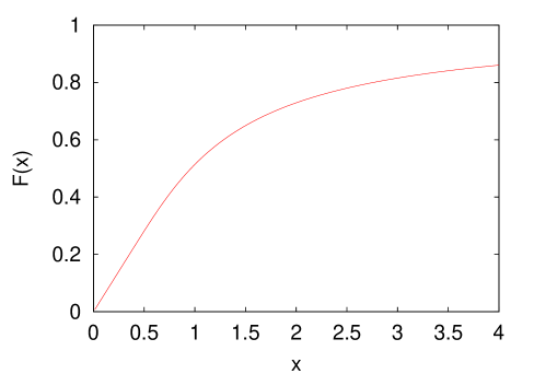
FIG. 1.: The function describing onset and saturation of the equilibrium fluctuation magnitude in a rapidity window with time: (23), (24).

III Realistic rescattering in hadronic gas

A Cascade estimates of the diffusion rates

Our estimates for $\Delta y_{\rm diff}$ in the hadronic gas phase can be simplified by noting that the dependence of $\gamma$ on $\tau$ in (16) is mostly due to $\tau_{\rm free}$. The rapidity change per collision, $\delta y_{\rm coll}$, is approximately independent of $\tau$, since the decrease of the temperature is relatively weak in the whole hadronic stage, $T=160-110$ MeV, and kinematics of low energy scattering changes little. In other words, $\Delta y_{\rm diff}$ is given by the random walk formula

$$\Delta y_{\rm diff}=\delta y_{\rm coll}\ \sqrt{N_{\rm coll}},$$ (25)

where

$$N_{\rm coll}=\int_{0}^{\tau}{d\tau\over\tau_{\rm free}},$$ (26)

is the total number of collisions per particle during the time $\tau$, from the beginning of the hadronic phase, $\tau=0$, until freeze-out.

At comparatively low relative energies of re-scattering in question, all relevant processes are due to certain resonances, such as $\Delta$ for $\pi N$ collisions, $\rho$ for $\pi\pi$ ones, etc. So, our first task is to determine what is the mean change of rapidity in such collisions. Taking pions and nucleons with thermal distribution, we have found probabilities of different resonances and have determined the following values for the mean rapidity shifts per collision

$$\delta y_{\rm coll}^{\pi}\approx 0.8;\qquad\delta y_{\rm coll}^{N}\approx 0.2.$$ (27)

The second (and much more involved) task is to evaluate the average number of re-scatterings, for each type of particles. The average value can be evaluated from standard rates

$$N^{i}_{\rm coll}=\sum_{j}\int dt\ \sigma_{ij}\,v_{ij}(t)\,n_{j}(t)$$ (28)

and even a very simple estimate shows that those numbers are not small. The nucleons suffer especially multiple collisions, of the order of 10-20, since the $\Delta$-induced cross section at its peak is as large as 200 mb, and there are many pions around. (This phenomenon is sometimes referred to as pion wind.) However, more accurate estimates depend on many details, like the geometrical location of the particle in question, expansion of the fireball etc. Those can only be obtained from either realistic hydro simulations or from hadronic cascades.

We have chosen the latter alternative, using two popular hadronic cascade codes. First, we have generated AuAu RHIC events (100+100 GeV) with RQMD[16], and looked at the total rescattering number per particle located at midrapidity $y\approx 0$. The results are shown in Fig.2, as a distribution over the number of rescatterings suffered by Kaons and Nucleons. One can see that for the nucleons the distribution has a very wide tail, reaching large values and with an average being of the order of 20. Kaons, on the other hand, suffer much smaller number of collisions, about 5 in average, and there is about 20% of kaons without rescattering at all.

Unfortunately standard RQMD output does not allow to trace an individual pion, which appears and disappears, and we do not have the mean rescattering pion number directly from that simulation. We can only evaluate the total number of $\pi-N$ rescatterings

$$N_{\rm coll}^{\pi}=N_{\rm coll}^{N}\cdot{\langle dN_{N}/dy\rangle\over\langle dN_{\pi}/dy\rangle}\approx 2,$$ (29)

but those are far from being dominant.

Fortunately, a similar code, UrQMD [17], has been extensively studied, and in the talk by M. Bleicher one finds a graph showing $dN_{\rm coll}/ds$ for baryon-baryon, baryon-meson and meson-meson collisions, under the same conditions. Dividing by the number of mesons and integrating over subcollision invariant energy, $s$, we obtained the total number of collisions from meson-meson scattering to be $N_{\rm coll}^{\rm meson}\approx 8$ per meson. Most of the mesons are pions, of course, and this number fits well between N and K ones mentioned above.

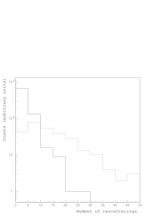
FIG. 2.: Distribution over the number of rescatterings in central AuAu 100+100 AGeV collisions, according to RQMD code. The solid line is for Kaons, the dashed one for Nucleons, both taken in the mid-rapidity region ($|y|<2$).

Adopting these numbers, we can combine it with rapidity change per scattering, and get our final estimates for the diffusion distance at RHIC:

$$\Delta y_{\rm diff}^{\pi}\approx 2.2;\qquad\Delta y_{\rm diff}^{N}\approx 0.9.$$ (30)

At SPS the pion multiplicity is about factor 2 smaller, and the rescattering number is reduced to $N_{\rm coll}^{N}\approx 15$ and $N_{\rm coll}^{\pi}\approx 5$, so that at SPS

$$\Delta y_{\rm diff}^{\pi}\approx 1.8;\qquad\Delta y_{\rm diff}^{N}\approx 0.77,$$ (31)

Let us now compare it to some typical experimental conditions at SPS. For the accepted interval of rapidity of $\Delta y=2$, the argument of $F(x)$ plotted in Fig.[1] is directly these values of $\Delta y_{\rm diff}$, and one can read $F$ from it: the result is 0.7 and 0.42 for pions and nucleons.

In the previous section we described an idealized case $\sigma_{k}^{2}(0)\ll\chi_{k}$. For our estimate of the effect we shall use more general expression, which gives the time dependence of $\langle(\Delta Q)^{2}\rangle$ given its initial value at the beginning of the hadronic phase, $\tau=0$, $\langle(\Delta Q)^{2}\rangle_{0}=\sigma_{0}^{2}(0)\Delta y$ and the hadronic gas equilibrium value $\langle(\Delta Q)^{2}\rangle_{\rm eq}=\chi_{0}\Delta y$:

$$\langle(\Delta Q)^{2}\rangle = \langle(\Delta Q)^{2}\rangle_{\rm eq}\ F(x)+\langle(\Delta Q)^{2}\rangle_{0}\ (1-F(x));$$ (33)

$$x={\Delta y_{\rm diff}\over(\Delta y/2)}.$$

For example, starting from the fluctuations suppressed by a factor of about 3 [10, 11], i.e., $\langle(\Delta Q)^{2}\rangle_{0}/\langle(\Delta Q)^{2}\rangle_{\rm eq}\approx 1/3$, and using $F\approx 0.70$ for the fluctuations of the electric charge we find: $\langle(\Delta Q)^{2}\rangle/\langle(\Delta Q)^{2}\rangle_{\rm eq}\approx 0.80$. I.e., only a 20% suppression survives until freeze-out after a 3-fold suppression at the QGP-hadron-gas transition. Similar estimate for the baryon number with $F\approx 0.42$, is more encouraging: $\langle(\Delta B)^{2}\rangle/\langle(\Delta B)^{2}\rangle_{\rm eq}\approx 0.62$.

B Charge fluctuations at SPS

We have shown above, that the pion diffusion in rapidity in the hadronic phase is sufficiently strong. For a typical detector with the acceptance $\Delta y=2$ it reduces the initial deviation from equilibrium value of event-by-event charge fluctuation to nearly its equilibrium value in the hadronic gas given by [7]

$${\langle(\Delta Q)^{2}\rangle\over\langle N_{\rm ch}\rangle}\approx 0.7,$$ (34)

which is very far from the QGP value. The deviation from the Poissonian value of 1 is due to the $\pi^{+}$, $\pi^{-}$ multiplicity correlation induced by resonance decays.

Furthermore, a specific centrality dependence of charge fluctuations in PbPb collisions follows from the resonance gas freezeout scenario. The magnitude of charge fluctuations (34) should increase towards most central collisions. This is opposite to what the QGP signal is supposed to do, if one expects it to show up in more central collisions.

This opposite trend is due to the fact that more central collisions correspond to lower freeze-out temperature [18]: the larger multiplicity is, the later freeze-out occurs. Significant centrality dependence of the radial flow observed at SPS confirms this idea. It follows, that for most central collisions one expects less resonances, and correspondingly decreased deviation of charge fluctuation from the Poissonian value 1.

A simple estimate of this effect can be made using the fact that the contribution of the resonances is controlled by the Boltzmann factor. Thus, for example, a decrease of temperature by $\Delta T\approx 20$ MeV leads to a decrease of the contribution of the $\rho_{0}$ resonance by a factor of 2. Similar decrease should occur in the contribution of other resonances, such as $\omega$. Therefore the variation with centrality of the freezeout temperature of order $20$ MeV would correspond to centrality dependence of (34) of the order of 10%, rising towards more central events.

C Charge fluctuations at RHIC

Finally, let us briefly discuss prospects of observation of QGP-like charge fluctuations at RHIC. STAR detector has significantly larger rapidity acceptance, and although diffusion of pions is slightly stronger at RHIC, one can hope to see deviations from the resonance gas value. Indeed, for the rapidity window $\Delta y=4$, equations (30), (33) predict that the primordial QGP factor 1/3 suppression of electric charge fluctuation will survive as factor

$${\langle(\Delta Q)^{2}\rangle\over\langle(\Delta Q)^{2}\rangle_{\rm eq}}\approx 0.7$$ (35)

suppression. Another important prediction is that this suppression must strengthen, i.e., the ratio (35) decrease, as the width $\Delta y$ is increased. In other words, opening wider rapidity “aperture” allows to see deeper back into the history of the collision.

The baryon number fluctuations have slower diffusion, but rapid proton-neutron conversion together with virtual invisibility of neutrons basically undermine the very idea: the relaxation slow-down can only occur if the current under consideration is a conserved one. Similar problem arises if one considers strangeness fluctuations.

IV $\pi^{+}/\pi^{-}$ fluctuations near the critical point $E$

In this section we discuss a new signature of the critical end-point $E$ [19] based on the $\pi^{+}/\pi^{-}$ fluctuations. As discussed in [19, 4], the main feature of thermodynamics near the critical point is the presence of long-wavelength fluctuations of the magnitude of the chiral condensate, or, the $\sigma$-field. One of the signatures proposed in [19, 4] was based on the fact that such light $\sigma$-quanta cannot decay at freeze-out, if it occurs near point $E$, and their large population survives until the time after freeze-out when their rising mass exceeds the 2$\pi$ threshold. The signature proposed in [19, 4] used the fact that produced pions had a necessarily non-thermal spectrum with low mean $p_{T}$.

The contribution of $\sigma$ decays to the pion spectrum is, to some extent, similar to contributions of other, standard, resonances in the resonance gas model, such as $\rho^{0}$. In particular, the produced $\pi^{+}\pi^{-}$ pairs introduce positive correlation between the numbers of positive and negative pions, therefore reducing the fluctuation of $\pi^{+}/\pi^{-}$ ratio. The most significant difference is that the contribution of $\sigma$ decays is only present near the critical point.

In order to estimate this contribution, we assume that the thermal population of $\sigma$’s is approximately half of the so-called “direct” charged pions (since the mass of the sigma is comparable to $m_{\pi}$), as is done in [4]. Thus the decaying $\sigma$’s produce the number of charged pions of order $2\times 2/3\times 1/2=2/3$ of the number of “direct” charged pions. The latter is about 1/3 of the total number, the rest are produced by resonance decays. Therefore, the contribution of sigmas to the charge pion multiplicity is about $2/3\times 1/3\approx 20\%$. Thus, the contribution of $\sigma$’s can be estimated to result in a reduction of fluctuations by an amount of order 20%.

Even though the actual contribution will also depend on the detector acceptance of the soft part of the pion spectrum, it is reasonable to expect a noticeable suppression, comparable to the suppression of about 30% due to standard resonances ($\rho^{0}$, $\omega$, etc.) in (34).

What is important is that such an additional suppression of the $\pi^{+}/\pi^{-}$ fluctuations can only appear if the freeze-out occurs near the critical point. As a function of the collision energy, this effect will be seen as a dip in the magnitude of the $\pi^{+}/\pi^{-}$ fluctuation, thus providing a signature for the discovery of $E$. Away from the critical point the fluctuations will be compatible with the ordinary resonance gas result calculated in [7].

The NA49 collaboration have now acquired data from collisions at 40, 80 and 160 AGeV of initial energy at SPS. We are looking forward to the analysis of this data. If it shows a monotonic dependence of $\pi^{+}/\pi^{-}$ ratio fluctuation on collision energy as well as on centrality, consistent with the resonance gas prediction, then one should be able to rule out the presence of the critical point in regions of the QCD phase diagram the location of which can be determined by the analysis similar to [20]. Collisions at other energies, in particular those of RHIC, will be needed to scan other regions of the phase diagram. If a signal described here is observed, other signatures discussed in [4] must also be seen to confirm the discovery of the critical point.

REFERENCES

- [1] L. Stodolsky, Phys. Rev. Lett. 75 (1995) 1044.
- [2] E. V. Shuryak, Phys. Lett. B423, 9 (1998) [hep-ph/9704456].
- [3] H. Appelshauser et al. [NA49 Collaboration], Phys. Lett. B459, 679 (1999) [hep-ex/9904014].
- [4] M. Stephanov, K. Rajagopal and E. Shuryak, Phys. Rev. D60, 114028 (1999) [hep-ph/9903292].
- [5] G. Baym and H. Heiselberg, Phys. Lett. B469, 7 (1999) [nucl-th/9905022].
- [6] G. V. Danilov and E. V. Shuryak, nucl-th/9908027.
- [7] S. Jeon and V. Koch, Phys. Rev. Lett. 83, 5435 (1999) [nucl-th/9906074].
- [8] E. Shuryak, Nucl. Phys. A661 (1999) 119c.
- [9] S.Mrowczynski, Phys. Lett. B314 118 (1993); Phys. Rev. C49 2191 (1994); Phys. Lett. B393 26 (1997).
- [10] M. Asakawa, U. Heinz and B. Muller, Phys. Rev. Lett. 85, 2072 (2000) [hep-ph/0003169].
- [11] S. Jeon and V. Koch, Phys. Rev. Lett. 85, 2076 (2000) [hep-ph/0003168].
- [12] M. Bleicher, S. Jeon and V. Koch, hep-ph/0006201.
- [13] H. Heiselberg and A. D. Jackson, nucl-th/0006021.
- [14] K. Fialkowski and R. Wit, hep-ph/0006023.
- [15] N. Sasaki, O. Miyamura, S. Muroya and C. Nonaka, hep-ph/0007121.
- [16] H. Sorge, Phys. Rev. C52, 3291 (1995) [nucl-th/9509007].
- [17] M. Belkacem et al., Phys. Rev. C58, 1727 (1998); M. Bleicher, Talk at Parkcity Workshop, March 2000.
- [18] C. M. Hung and E. Shuryak, Phys. Rev. C57, 1891 (1998) [hep-ph/9709264].
- [19] M. Stephanov, K. Rajagopal and E. Shuryak, Phys. Rev. Lett. 81, 4816 (1998) [hep-ph/9806219].
- [20] P. Braun-Munzinger, I. Heppe and J. Stachel, Phys. Lett. B465, 15 (1999) [nucl-th/9903010].