Event-by-Event Fluctuations from Decay of a Polyakov Loop Condensate

Abstract

A model for particle production at the deconfining phase transition in QCD is developed, as the semi-classical decay of a condensate for the Polyakov loop. In such a model, generically particle production, as measured on an event-by-event basis, exhibits significant deviations from statistical behavior.

The deconfined phase of QCD at high temperature may be produced in the collisions of large nuclei at high energies, such as at RHIC and LHC. The usual picture of the deconfined phase is of a weakly interacting gas of quasi-particles. While this picture applies (well) above the critical temperature, $T_{c}$, it may not be very useful near $T_{c}$. Recently, an effective theory which is better suited near $T_{c}$ was proposed; in a mean field approximation, the free energy is due to a potential for the Polyakov loop [1].

In this Letter we propose that if the mean field theory is correct, particle production at the phase transition is driven by coherent oscillations of the Polyakov loop condensate. This is very similar to particle production from preheating in inflationary models of the early universe [2]. For both inflation and the mean field theory of [1], the potential energy of the Polyakov loop dominates the total energy density, so that particle production can be estimated by semi-classical means. Particle production from a coherent source is observable by measuring fluctuations on an event-by-event basis, and differs from particle production by an incoherent, or statistical, source.

Many of the features of our model are similar to particle production in Disoriented Chiral Condensates (DCC’s) [3, 4]. Because pions are light, the chiral condensate in a DCC has a small energy density relative to the total energy density. Thus the number of produced particles from the DCC is small relative to the total, and the particles are produced in a narrow region of phase space, on top of a large, incoherent background. In contrast, in the present model essentially all of the energy of the deconfined phase is going into oscillations of the Polyakov loop, and thereby into pions. We stress that while the Polyakov loop is treated classically, the production of pions is quantum-mechanical.

We also contrast this with the conjectured critical end-point of the chiral phase transition in the plane of temperature, $T$, and (baryon) chemical potential, $\mu$ [5, 6]. Through critical fluctuations in the sigma field, a critical end-point will also generate non-statistical fluctuations. The critical end-point, however, only exists for a specific value of $T$ and $\mu$; it is necessary to ”tune” the collision parameters to reach this exceptional point. If the effective theory of [1] applies to QCD, however, it should apply, about the critical temperature, for a large range of chemical potentials near zero; there is no need for tuning. Further, critical fluctuations [5, 6] are necessarily largest about zero momentum. In contrast, in the present model the produced particles typically have momenta of order several hundreds of MeV, with significant fluctuations about that large momentum scale. Unlike a critical end-point, one should not cut on particles with low momentum; deviations from statistical behavior appear in the average pion momentum.

We begin by reviewing the mean field theory for the Polyakov loop [1], and then present an illustrative calculation of particle production. This calculation is not meant to be definitive, but merely to sketch how a classical condensate for the Polyakov loop might decay.

To understand the mean field theory, consider first an $SU(N)$ gauge theory not for three colors, but in the limit of a large number of colors, $N\rightarrow\infty$. As first observed by Thorn [7], in this case the free energy itself is an order parameter. For temperatures below the deconfining phase transition, confinement occurs, and the free energy is due exclusively to hadrons, such as glueballs. As color singlets, glueballs only contribute of order one to the free energy. We assume the usual, “quarkless” large $N$ limit, in which the number of light quark flavors, $N_{f}$, is held fixed as $N\rightarrow\infty$; then mesons also contribute of order one to the free energy.

In contrast, above $T_{c}$ deconfinement occurs, and gluons contribute $\sim N^{2}$ to the free energy; the quark contribution is suppressed, $\sim N^{2}(N_{f}/N)$. At very high temperature, by asymptotic freedom the behavior of the free energy can be computed perturbatively.

There is a puzzle, however. The free energy is a gauge invariant quantity, and so at any temperature, should be describable exclusively in terms of gauge invariant excitations. While the glueballs change their nature with temperature, they remain the dominant gauge invariant excitations. But if color singlet glueballs can only contribute of order one to the free energy, what is the term $\sim N^{2}$ in the free energy due to?

The only quantity which can provide such a contribution is an expectation value for the Polyakov loop:

$$\ell(x)=\frac{1}{N}\;{\rm tr}\left({\cal P}\exp\left(ig\int^{1/T}_{0}A_{0}(x,\tau)\,d\tau\right)\right)\;;$$ (1)

$\rm tr$ is the matrix trace, $\cal P$ is path ordering, and $g$ is the gauge coupling constant; $A_{0}(x,\tau)$ is the time component of the vector potential in the fundamental representation, at a spatial position $x$ and euclidean time $\tau$. At a temperature $T$, the Wilson line is defined in imaginary time; we assume that it can be generalized to real time, although its detailed form is as yet unknown [1]. The full thermal Wilson line is an $SU(N)$ matrix; its expectation value includes both color adjoint degrees of freedom, $\tilde{\ell}_{a}$, and a color singlet, $\ell$ [1]. The $\tilde{\ell}_{a}$’s transform under the $SU(N)$ gauge group, while the $\ell$’s only transform under a global $Z(N)$ symmetry. The $SU(N)$ Wilson lines, $\tilde{\ell}_{a}$, may be important in driving the transition first order when $N\geq 3$, but in a mean field approximation for the free energy, only the Polyakov loop, $\ell$, matter [1]. (Following standard convention, but contrary to [1], henceforth we refer to the $\ell$’s as $Z(3)$ Polyakov loops, and to the $\tilde{\ell}_{a}$’s as $SU(3)$ Wilson lines.)

As the Polyakov loop is a color singlet, its expectation value, $\ell_{0}=\langle\ell\rangle$, is gauge invariant. This vanishes in the confined phase, up to corrections $\sim N_{f}/N\sim 1/N$, and is nonzero above $T_{c}$. At infinite temperature, by asymptotic freedom we can ignore fluctuations in the gauge field, and $\ell_{0}\rightarrow 1$.

Thus the term $\sim N^{2}$ in the free energy is due exclusively to the potential for the Polyakov loop condensate, ${\cal V}(\ell)$. The free energy of glueballs and other gauge invariant excitations contribute $\sim 1$, while quarks contribute $\sim N^{2}(N_{f}/N)\sim N$.

Of course $N$ is not infinite in QCD, but three. At least for the free energy, perhaps large $N$ is a good guide to the behavior for $N=3$. If so, then in the high temperature phase of QCD, the free energy is — in a precise sense — dominated by gluons, through the potential for the Polyakov loop. This is supported by Lattice data, which finds that the free energy is much smaller at low, than at high, temperature [1].

There is one aspect of the deconfining phase transition for $N=3$ which is very different from $N=\infty$. General arguments and Lattice simulations [8] suggest that the deconfining transition is of first order when $N\geq 4$ (it may be strongly first order, although definitive results in the continuum limit are lacking). In contrast, the deconfining phase transition is of second order for two colors [9], and nearly second order for three colors [10]. Thus at least as far as the order of the deconfining transition in the pure glue theory is concerned, $N=3$ is “near” $N=2$, not $N=\infty$.

For $N=3$, the order of the transition does change with the addition of dynamical quarks; we assume, however, that even if the transition becomes crossover, that it remains nearly second order [1]. That is, we assume that Polyakov loops become light for some range of temperatures, which we define as $T_{c}$. This is crucial to our analysis, because when $\ell$ becomes light, it oscillates with large amplitude about its minimum, and drives particle production.

(As an aside, we note that the free energy need not be small in the low temperature phase of a gauge theory. Consider, for example, a generalized large $N$ limit, in which $N_{f}/N$ is held fixed as $N_{f}$ and $N\rightarrow\infty$. This large $N$ limit is “quarky”, as there are $\sim N_{f}^{2}$ color singlet hadrons. These hadrons generate a free energy which is of order $N^{2}\sim NN_{f}\sim N_{f}^{2}$ at any temperature. The Polyakov loop is also nonzero at any temperature, $\ell_{0}\sim N_{f}/N\neq 0$. Even though $\ell_{0}\neq 0$, perhaps the potential for the Polyakov loop continues to dominate the free energy. However, in this case, even near $T_{c}$ the Polyakov loop is never light.)

For three colors, the Polyakov loop $\ell$ is complex valued, and we take the potential

$${\cal V}(\ell)=\left(-\frac{b_{2}}{2}\,|\ell|^{2}-\frac{b_{3}}{6}(\ell^{3}+(\ell^{*})^{3})+\frac{1}{4}(|\ell|^{2})^{2}\right)\,b_{4}\,T^{4}\,;$$ (2)

$\ell_{0}(T)$ is the global minimum of ${\cal V}(\ell)$ at a temperature $T$. Again, we normalize $\ell_{0}\rightarrow 1$ as $T\rightarrow\infty$.

An important feature is that because the Polyakov loop is the trace of a phase factor, it is a dimensionless field; the only scale to make up the correct powers of dimension is the temperature. This accounts for the overall $T^{4}$ in ${\cal V}(\ell)$. The coefficients $b_{2}$, $b_{3}$, and $b_{4}$ are then fitted to agree with Lattice data for the pressure in the pure glue theory at $T\geq T_{c}$; the pressure for $T<T_{c}$ is taken to vanish. Of course the pressure in the pure glue theory is not the same as in QCD; for instance, the ideal gas value of the pressure changes with the addition of quarks. Lattice simulations have also shown that $T_{c}$ changes as well; with $2+1$ flavors one finds $T_{c}\sim 180$ MeV [10, 11]. Lattice simulations have demonstrated, however, that even with dynamical quarks, the pressure, divided by the ideal gas value, is a nearly universal function of $T/T_{c}$ [1, 11]. We use this remarkable property in our fit, taking $b_{2}(T/T_{c})$, and $b_{3}$, from the pure glue theory. The overall constant $b_{4}$ is rescaled by the ratio of the ideal gas terms between QCD, with three massless flavors, and the pure glue theory.

The pressure in the pure glue theory for $T>T_{c}$ [12] is described with the constant values $b_{3}=2$ and $b_{4}\approx 0.6061$. In QCD, we take the same value of $b_{3}$, and rescale $b_{4}$ by the appropriate ratio of ideal gas values, $b_{4}\approx 0.6061\cdot 47.5/16$. In the spirit of mean field theory, we take the same values for $b_{3}$ and $b_{4}$ below $T_{c}$. Below $T_{c}$, an approximate expression for the string tension is $\sigma(T)=1.21\sqrt{\sigma_{0}^{2}-0.99T^{2}/(0.41)^{2}}$ [13], where $\sigma_{0}$ is the zero temperature string tension, $=1$ GeV/fm. The mass of the Polyakov loop is then used to fix $b_{2}$, $m_{\ell}^{2}=(\sigma(T)/T)^{2}\propto-b_{2}b_{4}T^{2}$.

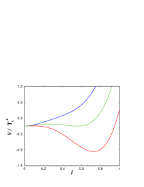
FIG. 1.: ${\cal V}(\ell)/T_{c}^{4}$ for temperatures $T/T_{c}=0.98$, 1, 1.02 (top to bottom), respectively.

In Fig. 1 we show ${\cal V}(\ell)$ in the vicinity of $T_{c}$, which is defined as the temperature were the two local minima of ${\cal V}(\ell)$ are degenerate. Notice that the potential changes extremely rapidly with temperature about $T_{c}$. This is due primarily to the rapid change of the coefficient $b_{2}$ with temperature. This can be seen either above or below $T_{c}$. Above $T_{c}$, the “bump” in the trace of the energy momentum tensor, times $1/T^{4}$, is due to the variation of $b_{2}$ [1]; it can also be seen from the extremely rapid decrease of the Debye screening mass, $\sim b_{2}$, from $2T_{c}$ to $T_{c}$, by a factor of ten [13]. Below $T_{c}$, $b_{2}$ changes rapidly because of the quick rise in the string tension as the temperature decreases [13]. Physically, this occurs because the Polyakov loop is light at $T_{c}$, and very heavy at zero temperature, $m_{\ell}(0)\geq 1.5$ GeV.

Except near the critical temperature, the Polyakov loop is heavy, so its fluctuations, and particle production, are small. Only near $T_{c}$ does the Polyakov loop become light and generate pions.

At $T_{c}$, because there is a first order transition, there are two degenerate minima, at $\ell=0$ and $\ell\approx 0.56$. As can be seen from the figure, however, the barrier between these two minima is small. This is because the pure glue theory has a weakly first order transition when $N=3$. It is so weak that this plays no part in our analysis. Thus whether the theory with dynamical quarks has a first order transition, or merely a crossover, is of little consequence; all that matters is that $\ell$ becomes light.

(The rapid variation of the potential with temperature, and the shallowness of the barrier between the two minima at $T_{c}$, is in contrast to models of the chiral transition [14]. For the chiral transition, the potentials change much more slowly with temperature, and the barriers to nucleation are significant; see, e.g., fig. (1) of [14].)

The complete effective theory is described by adding a kinetic term for $\ell$, and coupling it to a chirally symmetric field, $\phi$:

$${\cal L}\;=\;{\cal L}_{\phi}+\frac{N}{g^{2}}|\partial_{\mu}\ell|^{2}T^{2}-{\cal V}(\ell)-\frac{h^{2}}{2}{\phi}^{2}\;|\ell|^{2}T^{2}.$$ (3)

$\phi$ is the usual field describing pions and the sigma meson, with $O(4)$ global symmetry. The model can also be extended to three flavors, with kaons, etc.

Because the Polyakov loop is an effective field, normalized so that $\ell_{0}\rightarrow 1$ at high temperature, the coefficient of the kinetic term is not automatic. In the following analysis we require the coefficient of the kinetic term for the Polyakov loop, $\ell$, as it varys in time. We do not know this, so in (3) we take the coefficient of the kinetic term for $SU(3)$ Wilson lines, $\tilde{\ell}_{a}$, which vary in space [1]; we then assume a Lorentz invariant form to obtain the coefficient for time varying fields. While this is just a guess, taking $\alpha=g^{2}/(4\pi)=0.3$ at $T_{c}$ gives a coefficient $N/g^{2}\sim 0.8$, which is about unity and so reasonable.

The coupling constant for the Polyakov loop with mesons, $h^{2}$, could be fixed by knowing $\ell_{0}(T)$ and the meson masses above $T_{c}$. Since $\ell_{0}(T)$ is not known [1], our estimate is imprecise. Comparing to Lattice data of Gavai and Gupta for $m_{\pi}(T)$ at $T\geq T_{c}$ [15], $m_{\pi}/T=2\pi$ at $T\rightarrow\infty$ gives $h^{2}\approx 29$; at $T/T_{c}=2.9$, $m_{\pi}/T=4.29$, and the Hartree relation $m_{\pi}^{2}=\lambda^{2}(T^{2}/2-v^{2})+h^{2}T^{2}|\ell|^{2}$ (which follows from eqs. 3,4), yields $h^{2}=9$. In the actual calculations described below we employed $h^{2}=22$ as an intermediate value.

The lagrangian for the $\phi$ field is standard:

$${\cal L}_{\phi}\;=\;\frac{1}{2}(\partial_{\mu}{\phi})^{2}-\frac{\lambda^{2}}{4}\left({\phi}^{2}-v^{2}\right)^{2}+H\sigma\;.$$ (4)

At $T=0$ chiral symmetry is spontaneously broken, and the expectation values are $\langle\sigma\rangle=f_{\pi}$, $\langle\vec{\pi}\rangle=0$. Further, the PCAC relation gives $H=f_{\pi}m_{\pi}^{2}$, were $m_{\pi}=138$ MeV is the pion mass in the vacuum state at $T=0$. Then $v^{2}=f_{\pi}^{2}-m_{\pi}^{2}/\lambda^{2}$, and assuming a coupling $\lambda^{2}=20$ yields a sigma mass in vacuum of $m_{\sigma}^{2}=2\lambda^{2}f_{\pi}^{2}+m_{\pi}^{2}\approx(600$ MeV$)^{2}$.

There are many other terms which we could have included in the effective lagrangian. In particular, we really should have included terms linear in the Polyakov loop. In the pure glue theory, such terms are prohibited by the global $Z(3)$ symmetry of ’t Hooft, but it is expected to occur with dynamical quarks [16]. A term linear in the Polyakov loop will change the first order transition (in the pure glue theory) to crossover. We have ignored terms linear in the Polyakov loop because the free energy is small below $T_{c}$, so they must be small.

In this vein, we note the results of Digal, Laermann, and Satz [17]. They obtained Lattice results for two flavors of light, dynamical quarks. As expected for a second order chiral phase transition, about $T_{c}$ there is a peak in the chiral susceptibility, which becomes more pronounced as the quark mass decreases. For the range of quark masses studied, however, the peak in the susceptibility for the Polyakov loop also continues to grow. A term linear in the Polyakov loop should eventually cut off the divergence in the susceptibility for the Polyakov loop; thus their results also suggest that in the effective lagrangian, the effects of all terms linear in $\ell$ (times one, $\phi^{2}$, etc.) are small.

To compute particle production we take a simple dynamical picture. We assume an instantaneous quench from an initial temperature $T_{+}>T_{c}$, to a temperature $T_{-}<T_{c}$ [4]. We stress that because the $\ell$-potential varies so rapidly with temperature around $T_{c}$, the assumption of a quench appears natural. We then evolve the field, given its value for the minimum at $T_{+}$, with the potential at $T_{-}$. The $\ell$-field is no longer at a minimum at $T_{-}$, and so it rolls down the potential, and oscillates around the new minimum at $\ell_{0}=0$. These oscillations in $\ell$ couple to $\phi$, and thereby produce pions and sigmas. For the purposes of illustration we only include the production of pions, ignoring that of sigma mesons.

We perform the standard decomposition of the pion field in terms of creation and annihilation operators times adiabatic mode functions $\vec{\pi}_{k}(t)$ [2, 18]. The equation of motion for the mode functions is

$$\frac{d^{2}\vec{\pi}_{k}(t)}{dt^{2}} = -\Omega_{k}^{2}\vec{\pi}_{k}(t)\;,$$ (5)

$$\Omega_{k}^{2} = k^{2}+m_{\pi}^{2}+\lambda^{2}\langle\vec{\pi}^{2}(t)\rangle+h^{2}|\ell|^{2}T^{2}\;.$$ (6)

The effective pion mass is calculated assuming Hartree type factorization,

$$\vec{\pi}^{2}(t,\vec{x})\simeq\langle\vec{\pi}^{2}(t)\rangle$$ (7)

which requires a subtraction at $t=0$ [18]

$$\langle\vec{\pi}^{2}(t)\rangle = \int\frac{d^{3}k}{(2\pi)^{3}}|\vec{\pi}_{k}|^{2}$$ (9)

$$=d_{\pi}\int\frac{d^{3}k}{(2\pi)^{3}}\left(\frac{N_{k}(t)}{\Omega_{k}(t)}+\frac{1}{2\Omega_{k}(t)}-\frac{1}{2\Omega_{k}(t=0)}\right)\;.$$

$d_{\pi}=3$ counts the number of isospin states. Inserting a cutoff $\Lambda$, which is assumed to be larger than all other mass scales, gives

$$\langle\vec{\pi}^{2}(t)\rangle \simeq \frac{d_{\pi}}{8}\left[c_{0}^{2}\log\frac{4\Lambda^{2}}{c_{0}^{2}}-c_{t}^{2}\log\frac{4\Lambda^{2}}{c_{t}^{2}}\right]$$ (10)

$$+ d_{\pi}\int\frac{d^{3}k}{(2\pi)^{3}}\frac{{\cal N}_{k}}{\Omega_{k}}\;,$$ (11)

where $c_{0}^{2}=m_{\pi}^{2}+h^{2}|\ell(t=0)|^{2}T^{2}$ and $c_{t}^{2}=m_{\pi}^{2}+\lambda^{2}\langle\vec{\pi}^{2}(t)\rangle+h^{2}|\ell(t)|^{2}T^{2}$. In the above equations, ${\cal N}_{k}$ denotes the occupation number of a mode with given isospin and with momentum $k$, subtracted for vacuum fluctuations,

$${\cal N}_{k}=\frac{\Omega_{k}}{2}\left(\frac{|\dot{{\pi}}_{k}|^{2}}{\Omega_{k}^{2}}+|{\pi}_{k}|^{2}\right)-\frac{1}{2}\;.$$ (12)

As initial conditions we consider the case that the state at $t=0$ contains vacuum fluctuations only, such that $\vec{\pi}_{k}(t=0)=\sqrt{1/2\Omega_{k}(t=0)}$, $d\vec{\pi}_{k}(t=0)/dt=-i\sqrt{\Omega_{k}(t=0)/2}$, and ${\cal N}_{k}(t=0)=0$.

Similarly, in the classical equation of motion for the Polyakov loop, we include the backreaction from the produced pions in the Hartree approximation, replacing $\vec{\pi}^{2}(t,\vec{x})$ by $\langle\vec{\pi}^{2}(t)\rangle$ as given in (11). We neglect fluctuations of $\ell$ here, which should be a reasonable approximation as long as the energy of the produced pions is well below that for the Polyakov loop at $t=0$. Of course, a more refined treatment is necessary in order to trace the time evolution to the point where the coherent oscillation of $\ell$ has dissipated its entire energy into pions, since produced mesons will scatter off the Polyakov loop condensate and cause it to decohere.

We performed numerical simulations for the following values of the parameters: $\Lambda=10f_{\pi}\sim 1$ GeV, $T_{+}=1.02$, $T_{-}=0.975$. In preheating after inflation [2], the coupling constant is very small, $\sim 10^{-12}$, and the inflaton field oscillates many times. Particle production occurs continuously during these oscillations, and resonance bands develop for modes in phase with the driving inflaton field. In the present model, both the coupling of the Polyakov loop to pions, $h^{2}=22$, as well as the self coupling of the pions, $\lambda^{2}=20$, are large. Consequently pion production happens rather quickly, within a few oscillations.

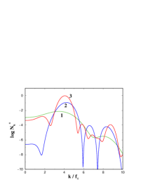
FIG. 2.: Occupation numbers of the pion modes at times $t=4n/3f_{\pi}$, for $n=1..3$.

In fig. 2 we show the logarithm of the produced pion occupation number versus momentum. The distribution exhibits less pronounced resonance bands than in the case where the contribution of fluctutations to $\Omega_{k}$ is neglected (compare also fig. 4 and fig. 5 in [19]). That is because $\lambda^{2}\langle\vec{\pi}^{2}(t)\rangle$ is time dependent, and shifts the resonance bands to other $k$ modes.

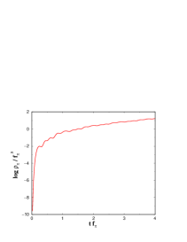
FIG. 3.: Pion density as a function of time.

Integrating over momentum,

$$\rho_{\pi}=\frac{d_{\pi}}{2\pi^{2}}\int_{0}^{\Lambda}dk\,k^{2}{\cal N}_{k}\;$$ (13)

we obtain the total density of produced pions. As shown in fig. 3, the pion density increases very rapidly: Parametric resonance lets the pion density increase exponentially over the depicted time interval.

The total pion density at time $t=4/f_{\pi}$ after the quench is approximately $\rho_{\pi}=0.35/$fm³. From $\rho_{\pi}$, the total number of pions per unit rapidity, $dN/dy$, is estimated as follows. Longitudinal length in the beam direction is a scale factor, $a$, times length in rapidity. For one dimensional Bjorken expansion [20], $a=\tau$, where $\tau$ is the proper time. If the expansion is isentropic, and $s$ is the entropy density, then $sa$ is a constant; taking $s\sim T^{3}$, a rough estimate of $a(T_{c})$ at RHIC is $\sim 10$ fm. Then $dN/dy=\rho_{\pi}\pi R^{2}a(T_{c})$. For a nucleus with $A\sim 200$, even without transverse expansion $R\simeq 7$ fm, so that $dN/dy\approx 1300\rho_{\pi}$ fm³ $\approx 460$. If transverse expansion increases $R$ by $50\%$, $dN/dy$ doubles and agrees roughly with data for central collisions at BNL-RHIC [21].

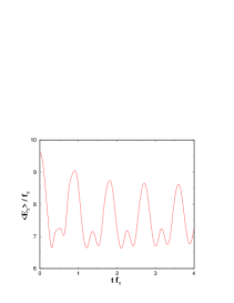
FIG. 4.: Mean energy per pion (in a given event and domain) as a function of time.

Fig. 4 shows the average energy per produced pion as a function of time. Unlike a thermal bath, the energy of all pions oscillates in phase with the background $\ell$-field, through the terms $\langle\vec{\pi}^{2}\rangle$ and $h^{2}|\ell|^{2}$. Because there is a lot of energy in the $\ell$-field, the pion energy is relatively large, and there are large fluctuations about the average. From Fig. 4, the time-averaged root-mean-square (RMS) fluctuation of the average pion momentum is $\sqrt{\langle p^{2}\rangle-\langle p\rangle^{2}}/\langle p\rangle\approx 10.3\%$. We have taken the ensemble average, i.e. the average over events, to be given by the time average from $t=0$ up to $t=4/f_{\pi}$.

This is our principal result. In a single domain, as for figs. 2 and 4, decay of a classical Polyakov loop condensate generates large fluctuations. In this picture, pions are produced in a pulse near $T_{c}$, from the “ringing” of the Wilson line into pions.

There are two effects which act to reduce the effect dramatically. First of all, experimentally it is necessary to average over many domains. The size of each domain is determined by how the quench ends, and involves both quantum mechanical and semi-classical processes. A lower bound for the size of a single domain is presumably given by the correlation length of the $\ell$-field at $T_{c}$, $\xi\sim 1/m_{\ell}(T_{c})$. From our estimates above, because $\ell$ becomes light at $T_{c}$, this correlation length is relatively large, $\xi\sim 1$ fm. Assuming one samples experimentally the full transverse size of the nucleus, and over one unit of rapidity, gives $N_{D}=\pi R^{2}a(T_{c})/(4\pi\xi^{3}/3)\sim 300$ domains. While perhaps semi-classical methods are suspect when each domain gives $\sim 1.5$ pions, if we average over $300$ domains, the RMS fluctuation of the average momentum per pion is reduced to $\sim 10.3\%/\sqrt{N_{D}}=0.6\%$. Averaging over many domains also acts to smooth out the momentum distribution of fig. 2, to leave a distribution which is closer to exponential.

While fluctuations $\sim 0.6\%$ are small, they are experimentally measurable. For central collisions at the CERN-SPS, $\surd{s}=18A$ GeV, the NA49 experiment compared the following two distributions of the average pion momentum [22, 6, 23]. The first was the event-by-event distribution of the actual data, the variance of which reflects intrinsic physical correlations in the event. The second is the same distribution in mixed events, constructed by picking particles at random from different events. The variance of mixed events is determined by purely statistical fluctuations, such as those due to finite particle number. To within $0.05\%$, however, the RMS fluctuations of the two distributions are the same.

Apparently, our model does not apply at SPS energies. One possibility is that the model is wrong. Another is that too large a region in rapidity, etc. was averaged over. It would be interesting to bin the data in increasingly small bins in rapidity, until one is limited by the usual statistical uncertainty, $\sim 1/\sqrt{N_{\Delta y}}$, where $N_{\Delta y}=(dN/dy)\Delta y$ is the number of particles in a rapidity bin of width $\Delta y$.

It is also possible that fluctuations at the SPS are washed out by scattering in a hadronic phase. We assume that particles produced at $T_{c}$ essentially flow to the detectors without further collisions, which is of course an idealized scenario. Collisions in a hadronic phase act to erase intrinsic fluctuations generated at $T_{c}$, and leave purely statistical fluctuations. We leave a detailed investigation of this point for future work. It is not clear, however, how easy it is for hadronic scattering to wash out fluctuations at $T_{c}$, due to expansion inherent in a heavy ion collision. Pions are nearly Goldstone bosons, whose scattering is suppressed at low energy by powers of momentum. For example, in model calculations [19], even though the self coupling of pions is large, pions can scatter into the zero mode of the pion field more rapidly than they can scatter out.

Our estimate of $dN/dy$ is just to tune the parameters of the model, but fluctuations in mean momentum $\sim 0.6\%$ should be a qualitatively correct prediction. Indeed, one can easily imagine how the fluctuations could even be larger. If the average size of the domains, $\xi$, is not $\sim 1$ but $\sim 2$ fm, then in one unit of rapidity there are only 40 domains instead of 300. Each domain generates about ten pions, and the RMS fluctuations of the average momentum per pion increases to $\sim 10.3\%/\sqrt{40}=1.7\%$. Notice, too, that as particle production increases exponentially in time, the distribution is dominated by those domains which last for the longest time.

If indeed hadron production at the confinement transition is dominated by the decay of a Polyakov loop condensate, we also expect nonstatistical (intrinsic) fluctuations of the pion multiplicity from event to event. For example, the RMS fluctuation of the multiplicity during the last 1 fm/c depicted in fig. 3 is $\sim 24\%$ in a single domain; for 300 domains, this gives fluctuations $\sim 1.4\%$.

Recently, fluctuations of the electric charge were analyzed [24]. Based upon a quasi-particle picture, it is argued that that RMS fluctuations of the charge, measured in a rapidity window $\Delta y\sim 1$, should be much smaller in a quark-gluon plasma than in a pion gas. Thus, if a thermal and locally neutral plasma were produced, and the pions emerged from the hadronization of that plasma with small relative rapidity, the charge fluctuations in the final state remain small: given a charged pion in $\Delta y$, the probability for its partner with opposite charge to have rapidity within $\Delta y$ is large. In the present model, on the other hand, pions produced from oscillations of the electrically neutral Polyakov loop are spread over a rapidity interval of $\sim\pm 2$ (see fig. 2), and the number of $\pi^{+}$ and $\pi^{-}$ in a given rapidity window $\Delta y\sim 1$ fluctuates independently. Thus, the RMS fluctuations of the charge should be large, i.e. like that of hadrons, not quarks.

The fluctuations are dominated by the behavior of the system as it goes through $T_{c}$. To first approximation, it does not matter how hot the system is initially. Consequently, the magnitude of the fluctuations should be approximately similar in collisions at RHIC and at the LHC. The only change with increasing the energy of the colliding nuclei is a change in the scale factor $a(T_{c})$, which produces a higher multiplicity at higher energy. As a constant number of pions is produced per domain, the width in rapidity should be chosen so that there is the same number of particles per rapidity bin. Higher energies can help, albeit indirectly: transverse expansion may be larger at higher energies, which prevents rescattering in the hadronic phase from washing out fluctuations induced at $T_{c}$.

We have made numerous approximations in the present analysis. A more careful study is certainly possible. The potential for the Polyakov loop in QCD, and the coupling to pions, can be computed from numerical simulations on the lattice, both without and with dynamical quarks. Many other improvements can also be made: introducing realistic models for the space-time dependence of the temperature, the effect of expansion in the equations of motion for $\ell$ and $\phi$, etc.

We have not attempted a better analysis here because STAR and other detectors will soon decide if heavy ion collisions at RHIC do or do not display intrinsic fluctuations on top of purely statistical fluctuations. We eagerly await this analysis.

Note added: After this paper was submitted for publication, many results were announced at Quark Matter 2001. CERES reported data from the SPS indicating fluctuations in the average transverse pion momentum $\sim 3\%$ [25]. At RHIC, STAR found that the same fluctuations appear to be much larger, $\sim 8\%$ [26]. STAR also reported that pion interferometry appears to indicate “explosive” behavior [26, 27]. We have recently suggested how the Polyakov loop model might generate explosive particle production and large fluctuations [28].

- [1] R. D. Pisarski, Phys. Rev. D62, 111501 (2000); hep-ph/0101168.
- [2] J. H. Traschen and R. H. Brandenberger, Phys. Rev. D42, 2491 (1990); L. Kofman, A. Linde and A. A. Starobinsky, Phys. Rev. D56, 3258 (1997).
- [3] A.A. Anselm, Phys. Lett. B217, 169 (1989); A.A. Anselm and M.G. Ryskin, Phys. Lett. B266, 482 (1991); J.-P. Blaizot and A. Krzywicki, Phys. Rev. D46, 246 (1992); J.D. Bjorken, Int. J. Mod. Phys. A7, 4189 (1992).
- [4] K. Rajagopal and F. Wilczek, Nucl. Phys. B404, 577 (1993).
- [5] M. A. Halasz, A. D. Jackson, R. E. Shrock, M. A. Stephanov and J. J. Verbaarschot, Phys. Rev. D58, 096007 (1998).
- [6] M. Stephanov, K. Rajagopal, and E. Shuryak, Phys. Rev. Lett. 81, 4816 (1998); Phys. Rev. D60, 114028 (1999); B. Berdnikov and K. Rajagopal, hep-ph/9912274.
- [7] C. B. Thorn, Phys. Lett. B99, 458 (1981); R. D. Pisarski, Phys. Rev. D29, 1222 (1984).
- [8] S. Ohta and M. Wingate, Nucl. Phys. Proc. Suppl. B73, 435 (1999); hep-lat/9909125; hep-lat/0006016.
- [9] J. Engels and T. Scheideler, Phys. Lett. B394, 147 (1997); Nucl. Phys. B539, 557 (1999).
- [10] F. Karsch, Nucl. Phys. Proc. Suppl. 83, 14 (2000).
- [11] F. Karsch, E. Laermann and A. Peikert, Phys. Lett. B478, 447 (2000).
- [12] B. Beinlich, F. Karsch, E. Laermann and A. Peikert, Eur. Phys. J. C6, 133 (1999).
- [13] O. Kaczmarek, F. Karsch, E. Laermann and M. Lutgemeier, Phys. Rev. D62, 034021 (2000).
- [14] O. Scavenius, A. Dumitru, E. S. Fraga, J. T. Lenaghan and A. D. Jackson, hep-ph/0009171.
- [15] R. V. Gavai and S. Gupta, hep-lat/0004011.
- [16] T. Banks and A. Ukawa, Nucl. Phys. B225, 145 (1983).
- [17] S. Digal, E. Laermann, and H. Satz, hep-ph/0007175; hep-lat/0010046.
- [18] D. Boyanovsky, H. J. de Vega, R. Holman and J. F. Salgado, Phys. Rev. D54, 7570 (1996); D. Boyanovsky, D. Cormier, H. J. de Vega, R. Holman, A. Singh and M. Srednicki, Phys. Rev. D56, 1939 (1997).
- [19] A. Dumitru and O. Scavenius, Phys. Rev. D62, 076004 (2000).
- [20] J. D. Bjorken, Phys. Rev. D27, 140 (1983).
- [21] B. B. Back et al. [PHOBOS Collaboration], hep-ex/0007036.
- [22] H. Appelshäuser et al. [NA49 Collaboration], Phys. Lett. B459, 679 (1999).
- [23] H. Heiselberg, nucl-th/0003046, and references therein.
- [24] M. Asakawa, U. Heinz and B. Müller, Phys. Rev. Lett. 85, 2072 (2000); S. Jeon and V. Koch, Phys. Rev. Lett. 85, 2076 (2000); H. Heiselberg and A. D. Jackson, nucl-th/0006021; M. Bleicher, S. Jeon and V. Koch, hep-ph/0006201.
- [25] H. Appelshäuser, to appear in the proceedings of Quark Matter 2001.
- [26] J. Harris, S. Panitkin, and J. Reid, to appear in the proceedings of Quark Matter 2001.
- [27] F. Laue and S. Panitkin, to appear in the proceedings of QM 2001.
- [28] A. Dumitru and R. D. Pisarski, hep-ph/0102020, to appear in the proceedings of QM 2001.