hep-ph/0010075 SLAC–PUB–8655

UCLA/00/TEP/26

October, 2000

Two-Loop Correction to Bhabha Scattering

Z. Bern^⋆

Department of Physics and Astronomy
UCLA, Los Angeles, CA 90095-1547

L. Dixon^†

Stanford Linear Accelerator Center
Stanford University
Stanford, CA 94309

and

A. Ghinculov^⋆

Department of Physics and Astronomy
UCLA, Los Angeles, CA 90095-1547

We present the two-loop virtual QED corrections to $e^{+}e^{-}\to\mu^{+}\mu^{-}$ and Bhabha scattering in dimensional regularization. The results are expressed in terms of polylogarithms. The form of the infrared divergences agrees with previous expectations. These results are a crucial ingredient in the complete next-to-next-to-leading order QED corrections to these processes. A future application will be to reduce theoretical uncertainties associated with luminosity measurements at $e^{+}e^{-}$ colliders. The calculation also tests methods that may be applied to analogous QCD processes.

Submitted to Physical Review D

  ^⋆Research supported by the US Department of Energy under grant DE-FG03-91ER40662. ^†Research supported by the US Department of Energy under grant DE-AC03-76SF00515.

1 Introduction

Bhabha scattering is an important process for extracting physics from experiments at electron-positron colliders primarily because it provides an effective means for determining luminosity. These measurements depend on having precise theoretical predictions for the Bhabha scattering cross sections. As yet, the complete next-to-next-to-leading order (NNLO) QED corrections needed for reducing theoretical uncertainties have not been computed. In this paper we present the complete two-loop matrix elements that would enter into such a computation. This calculation also provides a means for validating techniques that can be applied to physically important but more intricate QCD calculations. It also provides an additional explicit verification of a general formula due to Catani [1] for the structure of two-loop infrared divergences, and allows us to determine the process-dependent terms for the processes at hand.

In Bhabha scattering there are two distinct kinematic regions: small angle Bhabha scattering (SABS), and large angle (LABS). In the LEP/SLC energy range, SABS is used to measure the machine luminosity via a dedicated small angle luminosity detector. SABS has a large cross section — about four times larger than $Z$ decay in the $1^{\circ}-3^{\circ}$ window — making it particularly effective as a luminosity monitor. At the same time, SABS is calculable theoretically with high accuracy from known physics (mainly QED), apart from hadronic vacuum polarization corrections that rely upon the experimental data for $e^{+}e^{-}$ annihilation into hadrons at low energy [2, 3]. Therefore, SABS is an important ingredient in measuring any absolute cross section. For instance, the measurement of the hadronic cross section at the $Z$ peak, $\sigma_{\rm h}^{o}$, which enters several precision observables, is especially dependent on an accurate theoretical understanding of Bhabha scattering.

At LEP/SLC, large angle Bhabha scattering interferes with $e^{+}e^{-}\to Z\to e^{+}e^{-}$ and so it is needed to disentangle important parameters such as the electroweak mixing angle. It is also useful for measuring the luminosity at flavor factories such as BABAR, BELLE, DA$\Phi$NE, VEPP-2M, and BEPC/BES [4]. A peculiarity of future electron linear colliders is that the luminosity spectrum is not monochromatic because of the beam-beam effect. Because of this, measuring the total small angle cross section of Bhabha scattering alone is not sufficient, and therefore the angular distribution of LABS was proposed for disentangling the luminosity spectrum [5].

Due to the experimental importance of this process, significant effort has been devoted to developing Monte Carlo event generators — see for instance ref. [6] for an overview. In order to match the impressive experimental precision, a complete inclusion of NNLO QED quantum effects has become necessary. On the theoretical side, however, the calculation of two-loop four-point amplitudes has been a roadblock to further progress.

In this article we present the two-loop virtual QED corrections to the differential cross section for Bhabha scattering, i.e., the two-loop amplitude interfered with the tree amplitude and summed over all spins. We neglect the small electron mass in comparison to all other kinematic invariants, and use dimensional regularization to handle the ensuing infrared divergences. Besides these contributions, a number of other virtual and real emission contributions (discussed in the conclusions) still need to be obtained before a full Monte Carlo program for the Bhabha scattering cross section can be constructed.

The two-loop QED four-fermion amplitudes are also a useful testing ground for two-loop QCD calculations containing more than one kinematic invariant, which are required for higher-order jet cross sections and other aspects of collider physics. For processes that depend on a single momentum invariant, a number of important quantities have been calculated up to four loops, such as the total cross section for $e^{+}e^{-}$ annihilation into hadrons and the QCD $\beta$-function [7]. In contrast, the only complete two-loop four-point scattering amplitudes presently known for generic kinematics in massless gauge theory are the $N=4$ super-Yang-Mills amplitudes [8, 9], and $gg\to gg$ in a single helicity configuration in pure gauge theory [10]. The two-loop amplitudes required for NNLO computations of jet production in hadron colliders, or for NNLO three-jet rates and other event shape variables at $e^{+}e^{-}$ colliders, remain uncalculated. We note in passing that partial results for the leading-color part of two-loop contributions to quark-quark scattering have very recently appeared [11].

Two important technical breakthroughs are the calculations of the dimensionally regularized scalar double box integrals with planar [12] and non-planar [13] topologies and all external legs massless, and the development of reduction algorithms for the same types of integrals with loop momenta in the numerator (tensor integrals) [14, 15, 16, 17, 11]. Related integrals, which also arise in the reduction procedure, have been computed in refs. [18, 19]. Taken together, these results are sufficient to compute all loop integrals required for $2\rightarrow 2$ massless scattering amplitudes at two loops, thus removing a major obstacle to several types of NNLO calculations. In this paper we use these techniques to evaluate the integrals encountered in the Bhabha calculation. An even more recent result concerning two-loop planar double box integrals with one massive external leg [20] holds promise for the NNLO computation of three-jet rates at $e^{+}e^{-}$ colliders.

There has also been significant progress in developing general formalisms for other aspects of NNLO computations involving massless particles. The motivation has typically been infrared-safe observables in QCD, but many of the developments can be applied to the Bhabha process as well. The developments include an understanding of the intricate structure of the infrared singularities that arise when more than one particle is unresolved (i.e., is soft or collinear with another particle) [21, 22, 23]. Improved approximations to the NNLO correction to splitting functions have been constructed recently as well [24].

Infrared divergences are a significant complication in all the QCD and QED computations mentioned above. In any suitably “infrared-safe” observable all final-state divergences will cancel [25]. However, divergences occur in individual amplitudes for fixed particle number, and it is very useful to have a general description of such divergences. Catani has presented a general formula for the infrared divergence appearing in any two-loop QCD amplitude [1]. By appropriately adjusting group theory factors, it is straightforward to convert Catani’s QCD formula to a QED formula, allowing us to directly verify it. Moreover, we extract the exact form of a process-dependent term in the formula, for the case of QED scattering of four charged fermions. Previously, the only process for which this term had been extracted [1] was the quark form factor which enters Drell-Yan production [26]. (It should also now be possible to extract it for $gg\to$ Higgs using the recent two-loop computation [27].) Interestingly, a simple generalization of the quark form factor term (converted to QED) correctly predicts the process-dependent term for the $e^{+}e^{-}\to\mu^{+}\mu^{-}$ and Bhabha amplitudes. We also use Catani’s formula to conveniently organize the infrared divergences and to absorb some of the finite terms.

The previously computed non-abelian gauge theory amplitudes [8, 9, 10] were obtained via cutting methods. The low multiplicity and relative simplicity of the $e^{+}e^{-}\to\mu^{+}\mu^{-}$ and Bhabha scattering Feynman diagrams makes it relatively easy to directly compute the diagrams, as we do here. We include here only the pure QED diagrams, neglecting for example the contributions of $Z$ exchange, and hadronic vacuum polarization effects. The former are negligible at this order in SABS and in LABS at flavor factories. The hadronic contributions are important, but much of their effect is straightforward to include by introducing a running coupling.

We perform the calculation in dimensional regularization [28] with $d=4-2\epsilon$ and set the small electron mass to zero, since it is the only form in which the required two-loop momentum integrals are known. Moreover, it provides a powerful method for simultaneously dealing with both the infrared and ultraviolet divergences encountered in gauge theories. Traditionally, dimensional regularization is not used for QED, in part because the infrared divergences are relatively tame compared to non-abelian gauge theories, so photon and electron masses are sufficient for cutting off the theory. Another important reason for using dimensional regularization is to validate techniques that can also be applied to the more complicated case of QCD. In QCD, dimensional regularization is the universally utilized method for dealing with divergences.

In the high-energy Bhabha process, even with an “infrared-safe” (calorimetric) final-state definition, the electron mass will still appear in large logarithms of the form $L\equiv\ln(Q^{2}/m_{e}^{2})$ due to initial-state radiation. However, in the dimensionally regulated amplitudes these singularities (like all others) appear as poles in $\epsilon$. It may therefore be most convenient to handle the initial-state singularities using an electron structure function method [29] implemented in the $\overline{\rm MS}$ collinear factorization scheme.

In the next section we briefly describe our method for computing the two-loop amplitudes. Then we describe Catani’s formula for the divergence structure of the amplitudes, followed by a presentation of the finite (${\cal O}(\epsilon^{0})$) terms for both $e^{+}e^{-}\to\mu^{+}\mu^{-}$ and Bhabha scattering. In the final section we give our conclusions, including some discussion of the remaining ingredients still required for construction of a numerical program for Bhabha scattering at this order.

2 The Two-Loop Amplitudes

The 16 independent Feynman diagram topologies describing the two-loop QED corrections to $e^{+}e^{-}\to\mu^{+}\mu^{-}$ and Bhabha scattering are enumerated in fig. 1. In this figure we have suppressed the fermion arrows. After including the fermion arrows and distinct labels for the external legs, there are a total of 47 Feynman diagrams; however, many of these diagrams generate identical results. Of the 47 diagrams, 35 contain no fermion loop, 11 contain one fermion loop, and 1 contains two fermion loops. The Bhabha amplitude may be obtained from the $e^{+}e^{-}\to\mu^{+}\mu^{-}$ amplitude by adding to it the same set of diagrams, but with an exchange of one pair of external legs. The $e^{-}\mu^{-}\to e^{-}\mu^{-}$ and $e^{-}\mu^{+}\to e^{-}\mu^{+}$ amplitudes may, of course, be obtained by crossing.

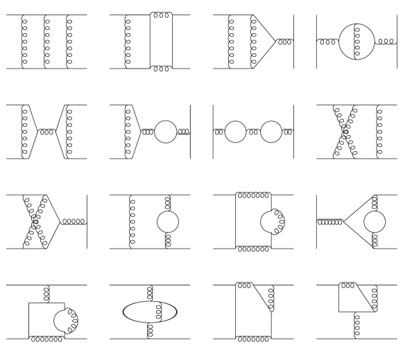
Figure 1: The independent diagrammatic topologies for two-loop four-fermion scattering in QED.

We have evaluated these diagrams interfered with the tree amplitudes and summed over spins in the conventional dimensional regularization (CDR) scheme. This interference gives directly the two-loop virtual correction to the $2\to 2$ differential cross section. The rules for implementing CDR are straightforward because all particle are treated uniformly in all parts of the calculation. In this scheme, all momenta and all Lorentz indices are taken to be $D=4-2\epsilon$ dimensional vectors. (The $\gamma$-matrices remain as $4\times 4$ matrices; i.e., ${\rm Tr}[1]=4$.)

After performing all $\gamma$-matrix algebra present in the two-loop Feynman diagrams, we use the conservation of momenta flowing on the internal lines to express the tensor structure of the diagrams in terms of inverse scalar propagators and a small number of additional scalar invariants containing loop momenta. The inverse scalar propagators cancel propagators in the denominator to generate simpler “boundary” integrals. To handle the integrals containing scalar invariants, we introduce Feynman parameters and interpret the resulting integrals in terms of scalar integrals with multiple propagators, which are then reduced to a set of master integrals with the help of equations in refs. [14, 15, 19].

Proceeding in this way, we obtain an expression for the amplitude in terms of master integrals (of the type listed in ref. [15], plus a few more for the planar double box topology) multiplied by coefficient functions. This expression is in principle valid to an arbitrary order in $\epsilon$, assuming that the master integrals could be evaluated to such an order. However, it is a bit too lengthy to present here, and for NNLO computations only the series expansion in $\epsilon$ through ${\cal O}(\epsilon^{0})$ is required. To carry out this expansion, we use expansions of the master integrals presented in refs. [12, 13, 14, 15, 18, 19]. As noted in ref. [11], there is a slight problem with the original choice of basis [14] for the two master planar double box integrals. In that basis, the coefficients for generic tensor integrals contain $1/\epsilon$ poles, necessitating an ${\cal O}(\epsilon)$ evaluation of the master integrals. Several solutions to this problem have been presented [17, 11]. We have used a slightly different solution, which is simply to use the original pair of master integrals defined in ref. [14], except evaluated in $d=6-2\epsilon$ instead of $d=4-2\epsilon$. In $d=6-2\epsilon$ the integrals have neither ultraviolet nor infrared divergences, making them simpler to evaluate through ${\cal O}(\epsilon^{0})$ than the $d=4-2\epsilon$ integrals.

Many of the master integral expansions quoted in refs. [12, 13, 14, 15, 18, 19] are in terms of Nielsen functions [30],

$$S_{n,p}(x)={(-1)^{n+p-1}\over(n-1)!\,p!}\int_{0}^{1}{dt\over t}\ln^{n-1}t\,\ln^{p}(1-xt)\,,$$

with $n+p\leq 4$. We have found it useful to express the results instead in terms of a minimal set of polylogarithms [31],

 

$${\mathop{\rm Li}\nolimits_{n}(x)}$$

 

with $n=2,3,4$, using relations such as

 

$${S_{13}(x)}$$

for

 

Here

$$\zeta_{s}\equiv\sum_{n=1}^{\infty}n^{-s}\,;\qquad\quad\zeta_{2}={\pi^{2}\over 6}\,,\qquad\zeta_{3}=1.202057\ldots,\qquad\zeta_{4}={\pi^{4}\over 90}\,.$$

The analytic properties of the non-planar double box integrals are somewhat intricate [13], since they are not real in any of the three kinematic channels for the $2\to 2$ process,

 

$${{}\hbox{$s$-channel}:\quad\,s>0;\quad t,\,u<0\,,}$$

 

where $s=(k_{1}+k_{2})^{2}$, $t=(k_{1}-k_{4})^{2}$, and $u=(k_{1}-k_{3})^{2}$. Therefore we shall present explicit formulae for the finite terms in the amplitude in both the $s$- and $u$-channels; those in the $t$-channel will be related by symmetries.

2.1 General Structure of Divergences

Dimensionally regulated two-loop amplitudes for four massless fermions contain poles in $\epsilon=(4-d)/2$ up to $1/\epsilon^{4}$. The structure of most of these singularities has already been exposed by Catani [1], who described the infrared behavior of general two-loop QCD processes. We shall therefore adopt his notation in presenting our results.

We work with ultraviolet renormalized amplitudes, and employ the $\overline{\rm MS}$ running coupling for QED, $\alpha(\mu^{2})$. Of course this scheme can always be converted to another one, for example $\alpha(Q^{2})$ defined via the photon propagator at momentum transfer $Q$, by a finite renormalization. The relation between the bare coupling $\alpha^{u}$ and $\alpha(\mu^{2})$ through two-loop order can be expressed as [1]

$$\alpha^{u}\,\mu_{0}^{2\epsilon}\,S_{\epsilon}\ =\ \alpha(\mu^{2})\,\mu^{2\epsilon}\Biggl{[}1-\alpha(\mu^{2}){\beta_{0}\over\epsilon}+\alpha^{2}(\mu^{2})\biggl{(}{\beta_{0}^{2}\over\epsilon^{2}}-{\beta_{1}\over 2\epsilon}\biggr{)}+{\cal O}(\alpha^{3}(\mu^{2}))\Biggr{]}\,,$$

where $S_{\epsilon}=\exp[\epsilon(\ln 4\pi+\psi(1))]$ and $\gamma=-\psi(1)=0.5772\ldots$ is Euler’s constant. The first two coefficients of the QED beta function are

$$\beta_{0}=-{N_{\!f}\over 3\pi}\,,\qquad\beta_{1}=-{N_{\!f}\over 4\pi^{2}}\,,$$

where $N_{\!f}$ is the number of light (massless) charge 1 fermions.

The renormalized four-fermion amplitude is expanded as

 

$${{\cal M}_{4}(\alpha(\mu^{2}),\mu^{2};\{p\})}$$

 

The infrared divergences of a renormalized two-loop amplitude in QCD or QED are [1],

 

$${|{\cal M}_{n}^{(2)}(\mu^{2};\{p\})\rangle_{{\scriptscriptstyle\rm R\!.S\!.}}}$$

 

where $|{\cal M}_{n}^{(L)}(\mu^{2};\{p\})\rangle_{{\scriptscriptstyle\rm R\!.S\!.}}$ is a color space vector representing the renormalized $L$ loop amplitude. The subscript ${\scriptscriptstyle\rm R\!.S\!.}$ stands for the choice of renormalization scheme, and $\mu$ is the renormalization scale. These color space vectors give the amplitudes via,

$${\cal M}_{n}(1^{a_{1}},\dots,n^{a_{n}})\equiv\langle a_{1},\dots,a_{n}\,|\,{\cal M}_{n}(p_{1},\ldots,p_{n})\rangle\,,$$

where the $a_{i}$ are color indices. The divergences of ${\cal M}_{n}$ are encoded in the color operators ${{\mbox{\boldmath$I$}}}^{(1)}(\epsilon,\mu^{2};\{p\})$ and ${{\mbox{\boldmath$I$}}}^{(2)}(\epsilon,\mu^{2};\{p\})$. In the QED case, the color space language is clearly unnecessary; ${\cal M}_{n}^{(L)}$ and ${{\mbox{\boldmath$I$}}}^{(L)}$ are just numbers.

In QCD, the operator ${{\mbox{\boldmath$I$}}}^{(1)}(\epsilon,\mu^{2};\{p\})$ is given by

$${{\mbox{\boldmath$I$}}}^{(1)}(\epsilon,\mu^{2};\{p\})=\frac{1}{2}{e^{-\epsilon\psi(1)}\over\Gamma(1-\epsilon)}\sum_{i=1}^{n}\,\sum_{j\neq i}^{n}\,{{\mbox{\boldmath$T$}}}_{i}\cdot{{\mbox{\boldmath$T$}}}_{j}\biggl{[}{1\over\epsilon^{2}}+{\gamma_{i}\over{{\mbox{\boldmath$T$}}}_{i}^{2}}\,{1\over\epsilon}\biggr{]}\biggl{(}\frac{\mu^{2}e^{-i\lambda_{ij}\pi}}{2p_{i}\cdot p_{j}}\biggr{)}^{\epsilon}\,,$$

where $\lambda_{ij}=+1$ if $i$ and $j$ are both incoming or outgoing partons and $\lambda_{ij}=0$ otherwise. The color charge ${{\mbox{\boldmath$T$}}}_{i}=\{T^{a}_{i}\}$ is a vector with respect to the generator label $a$, and an $SU(N_{c})$ matrix with respect to the color indices of the outgoing parton $i$. The values required for QCD are

 

$${{{\mbox{\boldmath$T$}}}_{q}^{2}}$$

 

For QED we let $C_{A}\to 0$, $C_{F}\to 1$, $T_{R}\to 1$ and ${{\mbox{\boldmath$T$}}}_{i}\cdot{{\mbox{\boldmath$T$}}}_{j}\to e_{i}e_{j}=\pm 1$, where the $e_{i}$ are the electric charges, to obtain

$${{\mbox{\boldmath$I$}}}^{(1)}(\epsilon,\mu^{2};\{p\})={e^{-\epsilon\psi(1)}\over\Gamma(1-\epsilon)}\biggl{(}{2\over\epsilon^{2}}+{3\over\epsilon}\biggr{)}\Biggl{[}-\biggl{(}{\mu^{2}\over-s}\biggr{)}^{\epsilon}-\biggl{(}{\mu^{2}\over-t}\biggr{)}^{\epsilon}+\biggl{(}{\mu^{2}\over-u}\biggr{)}^{\epsilon}\Biggr{]}\,,$$

for the four-fermion amplitude

$$e^{+}(k_{1})\,e^{-}(k_{2})\ \to\ \mu^{+}(k_{4})\,\mu^{-}(k_{3})\,.$$

(Note that the charges of incoming states should be reversed in computing ${{\mbox{\boldmath$T$}}}_{i}\cdot{{\mbox{\boldmath$T$}}}_{j}$.)

The operator ${{\mbox{\boldmath$I$}}}^{(2)}_{{\scriptscriptstyle\rm R\!.S\!.}}$ is given in QCD by [1]

 

$${{{\mbox{\boldmath$I$}}}^{(2)}_{{\scriptscriptstyle\rm R\!.S\!.}}(\epsilon,\mu^{2};\{p\})}$$

 

where the coefficient $K$ is:

$$K=\left(\frac{67}{18}-\frac{\pi^{2}}{6}\right)C_{A}-\frac{10}{9}T_{R}N_{\!f}\;\;.$$

For the QED process ($(2.14)$), we insert ${{\mbox{\boldmath$I$}}}^{(1)}$ from eq. ($(2.13)$), take $\beta_{0}$ and $\beta_{1}$ from eq. ($(2.7)$), and let $K\to-10N_{\!f}/9$.

The function ${{\mbox{\boldmath$H$}}}^{(2)}_{{\scriptscriptstyle\rm R\!.S\!.}}$ is process-dependent but has only single poles:

$${{\mbox{\boldmath$H$}}}^{(2)}_{{\scriptscriptstyle\rm R\!.S\!.}}(\epsilon,\mu^{2};\{p\})\ =\ {\cal O}(1/\epsilon)\,.$$

Ref. [1] does not give an expression for ${{\mbox{\boldmath$H$}}}^{(2)}_{{\scriptscriptstyle\rm R\!.S\!.}}$ for a general amplitude, but only for the case of a $q\bar{q}$ pair, i.e. a single charged fermion pair. The result, which is extracted from the two-loop QCD computation of the electromagnetic form factor of the quark [26], is

 

$${{{\mbox{\boldmath$H$}}}^{(2)}_{q\bar{q},{\scriptscriptstyle\rm CDR}}(\epsilon,\mu^{2};\{p\})}$$

 

where

$$\gamma_{(1)}\ =\ (-3+24\zeta_{2}-48\zeta_{3})C_{F}^{2}+\biggl{(}-{17\over 3}-{88\over 3}\zeta_{2}+24\zeta_{3}\biggr{)}C_{F}C_{A}+\biggl{(}{4\over 3}+{32\over 3}\zeta_{2}\biggr{)}C_{F}T_{R}N_{\!f}\,.$$

Performing the usual conversion to QED yields a result applicable to the electromagnetic form factor of the electron,

$${{\mbox{\boldmath$H$}}}^{(2)}_{e^{+}e^{-},{\scriptscriptstyle\rm CDR}}(\epsilon,\mu^{2};\{p\})={1\over 4\epsilon}{e^{-\epsilon\psi(1)}\over\Gamma(1-\epsilon)}\Biggl{(}{\mu^{2}e^{-i\lambda_{12}\pi}\over 2p_{1}\cdot p_{2}}\Biggr{)}^{2\epsilon}\biggl{[}-{3\over 4}+6\zeta_{2}-12\zeta_{3}+\biggl{(}-{25\over 27}+\zeta_{2}\biggr{)}N_{\!f}\biggr{]}\,.$$

Using our two-loop computation, and an all-orders-in-$\epsilon$ computation of the one-loop amplitude for $e^{+}e^{-}\to\mu^{+}\mu^{-}$ (see sect. 2.2), we have verified that the singular behavior of the $e^{+}e^{-}\to\mu^{+}\mu^{-}$ amplitude in CDR agrees precisely with that predicted by eq. ($(2.9)$) in all three kinematic channels. In addition, we have extracted the function ${{\mbox{\boldmath$H$}}}^{(2)}_{e^{+}e^{-}\mu^{+}\mu^{-},{\scriptscriptstyle\rm CDR}}$ controlling the $1/\epsilon$ poles in eq. ($(2.9)$). We obtain

 

$${{{\mbox{\boldmath$H$}}}^{(2)}_{e^{+}e^{-}\mu^{+}\mu^{-},{\scriptscriptstyle\rm CDR}}(\epsilon,\mu^{2};\{p\})}$$

 

This result agrees with a “naive” generalization from the form factor case, in which one sums eq. ($(2.20)$) over the six pairs of charged legs in the four-point amplitude, weighted by the sign of the charge product $e_{i}e_{j}$. (Note that the factors of $(\mu^{2}/(-s_{ij}))^{2\epsilon}$ are purely conventional here, since their deviation from unity only contributes at the level of finite parts, ${\cal O}(\epsilon^{0})$. However, the overall normalization is predicted correctly by the sum over the six pairs.)

2.2 $e^{+}e^{-}\to\mu^{+}\mu^{-}$ at One Loop to All Orders in $\epsilon$

In order to verify the structure of the infrared singularities, and to extract the finite remainder of the two-loop amplitude presented below, we computed the one-loop $e^{+}e^{-}\to\mu^{+}\mu^{-}$ amplitude (interfered with the tree amplitude) to all orders in $\epsilon$. The result is

$$\sum_{\rm spins}{\cal M}_{4}^{(1)}{\cal M}_{4}^{(0)\,\dagger}={2\over 3}{N_{\!f}\over\epsilon}\sum_{\rm spins}{\cal M}_{4}^{(0)}{\cal M}_{4}^{(0)\,\dagger}+\biggl{[}A^{(1)}+S\Bigl{[}A^{(1)}\Bigr{]}\biggr{]}\bigg{|}_{\xi=1}\,,$$

where the first term is the $\overline{\rm MS}$ counterterm, expressed in terms of the tree-level interference

$$\sum_{\rm spins}{\cal M}_{4}^{(0)}{\cal M}_{4}^{(0)\,\dagger}=8\biggl{[}{t^{2}+u^{2}\over s^{2}}\,-\,\epsilon\biggr{]}\ ,$$

and

 

$${A^{(1)}}$$

 

The symmetry operation $S$ acts as

$$S:\quad t\leftrightarrow u,\qquad\xi\leftrightarrow-\xi.$$

After carrying out the operation of $S$, one should then set $\xi=1$. (Basically, $\xi$ allows us to separate diagrams based on whether they have an even or odd number of photons attached to the muon line. Because photons have ${\rm C}=-1$, this criterion governs the $t\leftrightarrow u$ symmetry properties.)

In eq. ($(2.24)$), ${\rm Box}^{(6)}(s,t)$ and ${\rm Tri}(s)$ are one-loop box and triangle integrals, the former evaluated in an expansion around $d=6-2\epsilon$. For the divergence formula ($(2.9)$), we need their series expansions in $\epsilon$ through ${\cal O}(\epsilon^{2})$. In the $u$-channel, where the functions are manifestly real, their expansions are given by

 

$${{\rm Box}^{(6)}(s,t)}$$

 

where

$$v={s\over u}\,,\quad w={t\over u}\,,\quad V=\ln\biggl{(}-{s\over u}\biggr{)}\,,\quad W=\ln\biggl{(}-{t\over u}\biggr{)}\,.$$

The expansions in the $s$- and $t$-channels can be found using analytic continuation formulae such as [19]

 

$${\ln(1-x+i\varepsilon)}$$

 

where $i\varepsilon$ is an imaginary infinitesimal added to $s,t$ or $u$ before continuing.

We have verified that through $O(\epsilon^{0})$ our result for the one-loop amplitude agrees with a previous calculation [32], up to terms which can be identified as being due to the conversion between dimensional regularization and a photon mass regularization.

2.3 Modifications for Bhabha Scattering

In comparison with the process $e^{+}e^{-}\to\mu^{+}\mu^{-}$ described above, the Bhabha scattering process

$$e^{+}(k_{1})\,e^{-}(k_{2})\ \to\ e^{+}(k_{4})\,e^{-}(k_{3})\,,$$

has additional exchange diagrams. In general, the interference required for Bhabha scattering is given by

 

$${\sum_{\rm spins}{\cal M}_{4}^{(L_{1})}{\cal M}_{4}^{(L_{2})\,\dagger}\bigg{|}_{\rm Bhabha}\ }$$

 

where the symmetry $U$ acts as

$$U:\quad s\leftrightarrow t,$$

${\cal M}_{4}^{(L)}$ is the $L$-loop amplitude for $e^{+}e^{-}\to\mu^{+}\mu^{-}$, and $\tilde{\cal M}_{4}^{(L)}$ is the same $L$-loop amplitude but with legs 1 and 3 interchanged (taking into account the Fermi statistics minus sign).

2.4 Bhabha Scattering at One Loop to All Orders in $\epsilon$

In the CDR scheme, the tree-level exchange contribution required for Bhabha scattering in eq. ($(2.30)$) is

$$\sum_{\rm spins}{\cal M}_{4}^{(0)}\tilde{\cal M}_{4}^{(0)\,\dagger}=8\,(1-\epsilon)\biggl{[}{u^{2}\over st}+\epsilon\biggr{]}\,.$$

The one-loop exchange contribution, evaluated to all orders in $\epsilon$, is given by

$$\sum_{\rm spins}{\cal M}_{4}^{(1)}\tilde{\cal M}_{4}^{(0)\,\dagger}={2\over 3}{N_{\!f}\over\epsilon}\sum_{\rm spins}{\cal M}_{4}^{(0)}\tilde{\cal M}_{4}^{(0)\,\dagger}+\tilde{A}^{(1)}\ ,$$

where

 

$${\tilde{A}^{(1)}}$$

 

Using these results, and the computation of the two-loop exchange terms, we again find that the additional singular terms in Bhabha scattering are described by eq. ($(2.9)$), where (not surprisingly) ${{\mbox{\boldmath$H$}}}^{(2)}_{{\scriptscriptstyle\rm R\!.S\!.}}$ is given by precisely the same expression ($(2.21)$) that we found for $e^{+}e^{-}\to\mu^{+}\mu^{-}$.

2.5 Finite Contributions to the Amplitudes

2.5.1 $e^{+}e^{-}\to\mu^{+}\mu^{-}$

Finally we give the real (dispersive) part of the finite remainder in eq. ($(2.9)$), interfered with the tree amplitude in the CDR scheme. First we treat the $e^{+}e^{-}\to\mu^{+}\mu^{-}$ process ($(2.14)$). It is convenient to decompose the finite part according to the number of light flavors, $N_{\!f}$,

$$\sum_{\rm spins}{\rm Re}\Bigl{[}{\cal M}_{4}^{(2){\rm fin}}{\cal M}_{4}^{(0)\,\dagger}\Bigr{]}\ =\ 8\Bigl{[}F^{(0)}+N_{\!f}\,F^{(1)}+N_{\!f}^{2}\,F^{(2)}\Bigr{]}\,.$$

In the $s$-channel, the functions $F^{(i)}$ are given by

$$F^{(i)}\ =\ \biggl{[}F_{s}^{(i)}+S\Bigl{[}F_{s}^{(i)}\Bigr{]}\biggr{]}\bigg{|}_{\xi=1}\ ,$$

where

 

$${F_{s}^{(0)}\ }$$

 

 

$${F_{s}^{(1)}\ }$$

 

 

$${\hskip-199.16928ptF_{s}^{(2)}\ }$$

 

with

$$x={t\over s}\,,\quad y={u\over s}\,,\quad X=\ln\biggl{(}-{t\over s}\biggr{)}\,,\quad Y=\ln\biggl{(}-{u\over s}\biggr{)}\,,$$

and the symmetry operation $S$ is given in eq. ($(2.25)$).

In the $u$-channel, the $F^{(i)}$ are given by

$$F^{(i)}\ =\ F_{u}^{(i)}\Big{|}_{\xi=1}\ ,$$

where

 

$${F_{u}^{(0)}\ }$$

 

 

$${F_{u}^{(1)}\ }$$

 

$$\hskip-170.71652ptF_{u}^{(2)}\ =\ {4\over 9}(x^{2}+y^{2})\biggl{[}\ln^{2}(\mu^{2}/(-s))+{10\over 3}\ln(\mu^{2}/(-s))+{25\over 9}\biggr{]}\,.$$

Here $x$, $y$ are defined in eq. ($(2.40)$), whereas $v$, $w$, $V$, $W$ are defined in eq. ($(2.27)$).

In the $t$-channel, the functions $F^{(i)}$ are given by the action of the symmetry $S$ of eq. ($(2.25)$) on the $u$-channel results,

$$F^{(i)}\ =\ S\Bigl{[}F_{u}^{(i)}\Bigr{]}\Big{|}_{\xi=1}\,.$$

The two-loop virtual contribution to the $e^{+}e^{-}\to\mu^{+}\mu^{-}$ unpolarized cross section, restoring overall factors and averaging over initial spins, is given by

$${d\sigma^{(2)}\over dt}\ =\ {1\over 16\pi s^{2}}\times{(4\pi\alpha)^{2}\over 4}\times\Bigl{(}{\alpha\over 2\pi}\Bigr{)}^{2}\times 2\,\sum_{\rm spins}{\rm Re}\Bigl{[}{\cal M}_{4}^{(2)}{\cal M}_{4}^{(0)\,\dagger}\Bigr{]}\,.$$

2.5.2 Bhabha Scattering

For the finite two-loop remainder for the Bhabha scattering process ($(2.29)$), we quote only the $(s\leftrightarrow t)$ symmetric sum of the two exchange terms required by eq. ($(2.30)$). Again we decompose the answer according to $N_{\!f}$,

$$\sum_{\rm spins}\biggl{\{}{\rm Re}\Bigl{[}{\cal M}_{4}^{(2){\rm fin}}\tilde{\cal M}_{4}^{(0)\,\dagger}\Bigr{]}+U\biggl{[}{\rm Re}\Bigl{[}{\cal M}_{4}^{(2){\rm fin}}\tilde{\cal M}_{4}^{(0)\,\dagger}\Bigr{]}\biggr{]}\biggr{\}}\ =\ 8\Bigl{[}\tilde{F}^{(0)}+N_{\!f}\,\tilde{F}^{(1)}+N_{\!f}^{2}\,\tilde{F}^{(2)}\Bigr{]}\,.$$

In the $s$-channel, the functions $\tilde{F}^{(i)}$ are given by

$$\tilde{F}^{(i)}\ =\ \tilde{F}_{s}^{(i)},$$

where

 

$${\tilde{F}_{s}^{(0)}\ }$$

 

 

$${\tilde{F}_{s}^{(1)}\ }$$

 

$$\hskip-71.13188pt\tilde{F}_{s}^{(2)}\ =\ {4\over 9}{y^{2}\over x}\biggl{[}\ln^{2}(\mu^{2}/s)+\ln^{2}(\mu^{2}/(-t))+{10\over 3}\Bigl{(}\ln(\mu^{2}/s)+\ln(\mu^{2}/(-t))\Bigr{)}-\pi^{2}+{50\over 9}\biggr{]}\,,$$

and $x$, $y$, $X$, $Y$ are defined in eq. ($(2.40)$).

In the $t$-channel, the functions $\tilde{F}^{(i)}$ are given by the action of the symmetry $U$ of eq. ($(2.31)$) on the $s$-channel results,

$$\tilde{F}^{(i)}\ =\ U\Bigl{[}\tilde{F}_{s}^{(i)}\Bigr{]}\,.$$

In the $u$-channel, the functions $\tilde{F}^{(i)}$ are given by

$$\tilde{F}^{(i)}\ =\ \tilde{F}_{u}^{(i)}+U\Bigl{[}\tilde{F}_{u}^{(i)}\Bigr{]}\ ,$$

where

 

$${\tilde{F}_{u}^{(0)}\ }$$

 

 

$${\tilde{F}_{u}^{(1)}\ }$$

 

$$\hskip-199.16928pt\tilde{F}_{u}^{(2)}\ =\ {4\over 9}{y^{2}\over x}\biggl{[}\ln^{2}(\mu^{2}/(-s))+{10\over 3}\ln(\mu^{2}/(-s))+{25\over 9}\biggr{]}\,.$$

Here $x$, $y$ are defined in eq. ($(2.40)$), whereas $v$, $w$, $V$, $W$ are defined in eq. ($(2.27)$).

2.6 Checks on the Result

We performed several checks on our calculation. The calculation was performed with the computer algebra programs Maple, Mathematica, and FORM. To check the code, large parts of the calculation were performed independently with alternative programs written in different languages. Various checks were applied to the integral reduction procedures described in refs. [12, 13, 14, 15, 18, 19] and our implementation of them. For example, we reproduced the double box ultraviolet divergences in $d=8$ and $d=10$ reported in ref. [9], and several other previously calculated double box integrals [10]. An additional check on the non-planar tensor integrals is that unphysical $1/(t-u)$ poles occur in the representation of these integrals in terms of the master integral basis we used [15]; however, in the series expansion in $\epsilon$ such poles drop out after delicate cancellations between the various terms.

We checked the gauge invariance of the scattering amplitude by explicitly calculating the Feynman diagrams in a general $\xi$ gauge and observing that the gauge dependence drops out in the final result. This provides a non-trivial check of the diagrams and parts of the integral reduction procedure.

A strong check on the final result is provided by the matching of the IR divergence structure of the two-loop scattering amplitude with Catani’s formula ($(2.9)$), as discussed in sect. 2.1. A given integral will contribute to both infrared divergences and to finite terms. Thus a check of the divergent terms provides an indirect check that the finite terms have been correctly assembled.

Finally, we observed for small scattering angles a suppression of the leading logarithms, $\ell\equiv\ln(\theta^{2}/4)$, e.g. in the limit $s\to 0$ in the $t$-channel for process ($(2.14)$). In other small-angle limits (those not enhanced by the photon propagator pole) the leading power-law behavior is of course less singular, but it is dressed by large logarithms of the type $\ell^{4}$ and $N_{\!f}\ell^{3}$. But in the $t$-channel $s\to 0$ limit it cancels down to $\ell^{2}$ and $N_{\!f}\ell$. This behavior is in accord with a generalized eikonal representation for small-angle scattering [2].

3 Conclusions

In this paper we presented the two-loop QED corrections to $e^{+}e^{-}\rightarrow\mu^{+}\mu^{-}$ and to Bhabha scattering. We presented the results in terms of two-loop amplitudes interfered with tree amplitudes and summed over spins in the context of conventional dimensional regularization. In these results we have set the small electron and muon masses to vanish. (This is an excellent approximation for the highest energy current and future electron-positron colliders.)

The two-loop amplitudes presented in this paper are infrared divergent. To make use of them in a Monte Carlo program for the NNLO terms in the cross section, they must be combined with lower-loop matrix elements including photon emission, which should be computed using conventional dimensional regularization, at least in the singular regions of phase space. In particular, the pieces that need to be computed (for the Bhabha case) are

• the $e^{+}e^{-}e^{+}e^{-}$ one-loop amplitude interfered with itself.

• the $e^{+}e^{-}e^{+}e^{-}\gamma$ one-loop amplitude interfered with a five-point tree amplitude, and

• the $e^{+}e^{-}e^{+}e^{-}\gamma\gamma$ tree-level squared matrix element,

The interference of the dimensionally regularized one-loop four-point amplitude with itself does not appear to be in the literature. Nevertheless, it should be relatively straightforward to obtain, given that it involves only one-loop amplitudes with four-point kinematics. The required integrals are given to sufficiently high order in $\epsilon$ in eq. ($(2.26)$).

The QED one-loop five-point amplitude interfered with the five-point tree is a rather involved object to compute from scratch. However, the closely related one-loop helicity amplitudes for one photon and two quark pairs are known [33, 34, 35], and it is a relatively simple matter to modify the color factors to obtain the corresponding QED amplitudes. The one-loop helicity amplitudes are in the ’t Hooft-Veltman scheme. They can be converted to conventional dimensional regularization by altering the tree amplitude appearing in the coefficient of their singular terms [36]. Thus the $e^{+}e^{-}\mu^{+}\mu^{-}\gamma$ and $e^{+}e^{-}e^{+}e^{-}\gamma$ one-loop amplitudes may be extracted from the known literature through ${\cal O}(\epsilon^{0})$.

Because of the $1/\epsilon^{2}$ infrared divergences that are encountered in the phase-space integral, in regions where the photon is soft or collinear, one might seem to require the one-loop five-point amplitude through ${\cal O}(\epsilon^{2})$. However, this is not necessary [21]. Instead, one can replace the five-point amplitudes in singular phase-space regions by a combination of four-point amplitudes (which are given in this paper to the required order in the dimensional regularization parameter) and splitting amplitudes [37, 38]. The one-loop splitting amplitudes for QCD are enumerated to the required order in refs. [21]; the case of QED follows as usual by an appropriate conversion of color factors.

The tree-level helicity amplitudes for $e^{+}e^{-}\mu^{+}\mu^{-}\gamma\gamma$ and $e^{+}e^{-}e^{+}e^{-}\gamma\gamma$ have been known for a while [39]. (They also can be converted from the four-quark two photon amplitudes in ref. [35], for example.) In infrared-divergent regions of phase space one must include higher order in $\epsilon$ contributions from the matrix elements. Systematic discussion of these regions, where two particles can be soft or three collinear, has been presented in refs. [22] for the case of QCD. Once again the results for QED can be obtained by a conversion of the color factors.

Even with all of these matrix element ingredients assembled, it is a nontrivial task to devise a numerically stable method for carrying out the singular phase-space integrations. Nevertheless, this task is very analogous to that required to obtain QCD jet predictions at next-to-next-to-leading order, so it is likely that it will be attacked soon.

Besides the obvious application of the present paper to refined theoretical predictions for Bhabha scattering and for electron-positron annihilation into muons, it also serves as a further test of methods that can be applied to analogous QCD processes. We are confident that many more multi-particle two-loop amplitudes will be calculated before long.

References

[1]
S. Catani,
Phys. Lett. B427, 161 (1998) [hep-ph/9802439].
[2]
A.B. Arbuzov, V.S. Fadin, E.A. Kuraev, L.N. Lipatov, N.P. Merenkov
and L. Trentadue,
Nucl. Phys. B485, 457 (1997)
[hep-ph/9512344].
[3]
G. Montagna, M. Moretti, O. Nicrosini, A. Pallavicini and F. Piccinini,
Nucl. Phys. B547, 39 (1999)
[hep-ph/9811436];
B. F. Ward, S. Jadach, M. Melles and S. A. Yost,
Phys. Lett. B450, 262 (1999)
[hep-ph/9811245].
[4]
C.M. Carloni Calame, C. Lunardini, G. Montagna, O. Nicrosini and F. Piccinini,
Nucl. Phys. B584, 459 (2000)
[hep-ph/0003268].
[5]
M.N. Frary and D.J. Miller,
in Proceedings, Collisions at 500-GeV, pt. A
(Munich/Annecy/Hamburg 1991), report DESY 92-123A, p, 379;
N. Toomi, J. Fujimoto, S. Kawabata, Y. Kurihara and T. Watanabe,
Phys. Lett. B429, 162 (1998).
[6]
Reports of the Working Group on Precision Calculations for the
Resonance, CERN yellow report 95-03 (1995), part 3.
[7]
S.G. Gorishnii, A.L. Kataev and S.A. Larin,
Phys. Lett. B259, 144 (1991);
L.R. Surguladze and M.A. Samuel,
Phys. Rev. Lett. 66, 560 (1991),
err. ibid.66, 2416 (1991);
T. van Ritbergen, J.A. Vermaseren and S.A. Larin,
Phys. Lett. B400, 379 (1997)
[hep-ph/9701390].
[8]
Z. Bern, J.S. Rozowsky and B. Yan,
Phys. Lett. B401, 273 (1997)
[hep-ph/9702424].
[9]
Z. Bern, L. Dixon, D.C. Dunbar, M. Perelstein and J.S. Rozowsky,
Nucl. Phys. B530, 401 (1998)
[hep-th/9802162].
[10]
Z. Bern, L. Dixon and D.A. Kosower,
JHEP 0001, 027 (2000)
[hep-ph/0001001].
[11]
E.W.N. Glover and M.E. Tejeda-Yeomans,
hep-ph/0010031.
[12]
V.A. Smirnov,
Phys. Lett. B460, 397 (1999)
[hep-ph/9905323].
[13]
J.B. Tausk,
Phys. Lett. B469, 225 (1999)
[hep-ph/9909506].
[15]
C. Anastasiou, T. Gehrmann, C. Oleari, E. Remiddi and J.B. Tausk,
Nucl. Phys. B580, 577 (2000)
[hep-ph/0003261].
[16]
T. Gehrmann and E. Remiddi,
Nucl. Phys. B580, 485 (2000)
[hep-ph/9912329].
[17]
T. Gehrmann and E. Remiddi,
Nucl. Phys. Proc. Suppl. 89, 251 (2000)
[hep-ph/0005232];
C. Anastasiou, J. B. Tausk and M. E. Tejeda-Yeomans,
Nucl. Phys. Proc. Suppl. 89, 262 (2000)
[hep-ph/0005328].
[18]
C. Anastasiou, E.W.N. Glover and C. Oleari,
Nucl. Phys. B565, 445 (2000)
[hep-ph/9907523].
[19]
C. Anastasiou, E.W.N. Glover and C. Oleari,
Nucl. Phys. B575, 416 (2000)
[hep-ph/9912251].
[20]
V.A. Smirnov,
hep-ph/0007032;
T. Gehrmann and E. Remiddi,
hep-ph/0008287.
[21]
Z. Bern and G. Chalmers,
Nucl. Phys. B447, 465 (1995)
[hep-ph/9503236];
Z. Bern, V. Del Duca and C.R. Schmidt,
Phys. Lett. B445, 168 (1998)
[hep-ph/9810409];
D.A. Kosower and P. Uwer,
Nucl. Phys. B563, 477 (1999)
[hep-ph/9903515];
Z. Bern, V. Del Duca, W.B. Kilgore and C.R. Schmidt,
Phys. Rev. D60, 116001 (1999)
[hep-ph/9903516];
S. Catani and M. Grazzini,
hep-ph/0007142.
[22]
J.M. Campbell and E.W.N. Glover,
Nucl. Phys. B527, 264 (1998)
[hep-ph/9710255];
S. Catani and M. Grazzini,
Phys. Lett. B446, 143 (1999)
[hep-ph/9810389];
Nucl. Phys. B570, 287 (2000)
[hep-ph/9908523].
[23]
A. Gehrmann-De Ridder and E.W.N. Glover,
Nucl. Phys. B517, 269 (1998)
[hep-ph/9707224].
[24]
W.L. van Neerven and A. Vogt,
Phys. Lett. B490, 111 (2000)
[hep-ph/0007362];
A. Retey and J.A.M. Vermaseren,
hep-ph/0007294.
[25]
T. Kinoshita,
J. Math. Phys. 3, 650 (1962);
T.D. Lee and M. Nauenberg,
Phys. Rev. 133, B1549 (1964);
J. Collins, D. Soper and G. Sterman, in Perturbative QCD, edited by
A.H. Mueller (World Scientific, Singapore, 1989), and references therein.
[26]
R.J. Gonsalves,
Phys. Rev. D28, 1542 (1983);
G. Kramer and B. Lampe,
Z. Phys. C34, 497 (1987),
err. ibid.C42, 504 (1989);
T. Matsuura and W.L. van Neerven,
Z. Phys. C38, 623 (1988);
T. Matsuura, S.C. van der Marck and W.L. van Neerven,
Nucl. Phys. B319, 570 (1989).
[27]
R.V. Harlander,
hep-ph/0007289.
[28]
G. ’t Hooft and M. Veltman,
Nucl. Phys. B44, 189 (1972).
[29]
V.N. Baier, V.S. Fadin and V.A. Khoze,
Nucl. Phys. B65, 381 (1973);
G. Montagna, F. Piccinini and O. Nicrosini,
Phys. Rev. D48, 1021 (1993).
[30]
See e.g. K.S. Kölbig,
SIAM J. Math. Anal. 17, 1232 (1986).
[31]
L. Lewin, Dilogarithms and Associated Functions
(Macdonald, 1958).
[32]
W. Beenakker, F.A. Berends and S.C. van der Marck,
Nucl. Phys. B349, 323 (1991).
[33]
Z. Kunszt, A. Signer and Z. Trócsányi,
Phys. Lett. B336, 529 (1994)
[hep-ph/9405386].
[34]
A. Signer,
Phys. Lett. B357, 204 (1995)
[hep-ph/9507442].
[35]
V. Del Duca, W.B. Kilgore and F. Maltoni,
Nucl. Phys. B566, 252 (2000)
[hep-ph/9910253].
[36]
Z. Kunszt, A. Signer and Z. Trócsányi,
Nucl. Phys. B411, 397 (1994)
[hep-ph/9305239];
S. Catani, M.H. Seymour and Z. Trócsányi,
Phys. Rev. D55, 6819 (1997)
[hep-ph/9610553].
[37]
Z. Bern, L. Dixon, D.C. Dunbar and D.A. Kosower,
Nucl. Phys. B425, 217 (1994)
[hep-ph/9403226].
[38]
Z. Bern, L. Dixon and D.A. Kosower,
Nucl. Phys. B437, 259 (1995)
[hep-ph/9409393].
[39]
F. A. Berends, P. De Causmaecker, R. Gastmans, R. Kleiss, W. Troost and
T.T. Wu,
Nucl. Phys. B264, 265 (1986);
J. F. Gunion and Z. Kunszt,
Phys. Lett. B176, 477 (1986).