Perturbative QCD analysis of near-to-planar three-jet events.

Abstract

We present the all-order resummed $K_{\mbox{\scriptsize out}}$ distribution as a measure of aplanarity in three-jet events.

1 Introduction

In recent years much theoretical and experimental effort has been devoted to the study of the so-called jet-shape variables. Such observables are useful to describe the spatial distribution of final state particles in high energy hadronic processes, like $e^{+}e^{-}$ annihilation and DIS. For many of these (e.g. thrust and heavy-jet mass [1], C-parameter [2] and the jet Broadenings [3]) perturbative (PT) distributions are already available, and it is even possible to estimate the power-suppressed corrections due to confinement effects (for reviews see[4],[5]).

For two-jet configurations, the kinematical region in which the two jets are “pencil-like” turns out to be particularly interesting , since here multiple soft gluon radiation effects become essential. We meet an analogue of this situation for three-jet events if we study near-to-planar configurations. The variable we choose as a measure of event aplanarity is $K_{\mbox{\scriptsize out}}$, defined as the sum of the moduli of the momenta lying out of the event plane.

The aim of this paper is to present the main features of $K_{\mbox{\scriptsize out}}$ perturbative distribution, while all computational details may be found in [6].

The calculation is performed at the “state of art” level, which means all-order resummation of double- (DL) and single-logarithmic (SL) contributions due to soft and collinear gluon radiation effects, two-loop analysis of gluon radiation probability and matching the resummed logarithmic expressions with the exact ${\cal{O}}\left(\alpha_{\mbox{\scriptsize s}}^{2}\right)$ results.

In Section 2 basic definitions and notations are introduced, together with a discussion on the sources of SL corrections. These are examined in detail in Section 3 , which contains the complete expression for $K_{\mbox{\scriptsize out}}$ distribution to SL accuracy. Gluon radiation effects are included in the so-called “radiator”, which is described in Section 4. In Section 5 is shown the final answer for the distribution. We finally draw some conclusions and present further developments of our research (Section 6).

2 Definition of the observable

As it is known, a three-jet event in $e^{+}e^{-}$ annihilation is generated by a quark-antiquark pair which radiates a hard gluon. For kinematical reasons these three partons lie in a plane. When additional partons are emitted this is no longer true, but it is still possible to define an event-plane and to measure the radiation out of this plane.

First we introduce the thrust and thrust-major of the event ($Q$ is the $e^{+}e^{-}$ centre-of-mass energy),

$$T\,Q=\max_{\vec{n}}\left\{\sum_{h}\left|\>\vec{n}\vec{p}_{h}\>\right|\right\}\>=\>\sum_{h}\left|\>{p}_{hz}\>\right|\>,$$ (1)

$$T_{M}\,Q=\max_{\vec{n}\vec{n}_{T}=0}\left\{\sum_{h}\left|\>\vec{n}\vec{p}_{h}\>\right|\right\}\>=\>\sum_{h}\left|\>{p}_{hy}\>\right|\>.$$ (2)

We choose to fix the $z$ and $y$ axis along the thrust and thrust-major axis respectively. Orientation of these two axes is determined by imposing that the momentum of the most energetic particle has a positive $z$-component, while the momentum of the second most energetic particle has a positive $y$ component. Hereafter we attribute $p_{h}$ to the right hemisphere (left hemisphere ) if $p_{hz}>0$ ($p_{hz}<0$). Similarly $p_{h}$ is in the up hemisphere (down hemisphere) if $p_{hy}>0$ ($p_{hy}<0$). The $T$-$T_{M}$ plane is called the event plane, and the sum of the moduli of the out-of-plane momenta gives the thrust-minor:

$$T_{m}\,Q=\sum_{h}\left|\>{p}_{hx}\>\right|\>\equiv\>K_{\mbox{\scriptsize out}}\>.$$ (3)

Such definitions, together with energy-momentum conservation, force the transverse momentum with respect to the thrust axis $k_{t}\equiv(k_{x},k_{y})$ to be conserved separately in the right and left hemisphere. Similarly the $x$-component of $k_{t}$ is conserved independently in the up and down hemisphere.

Near-to-planar three-jet events belong to the kinematical region $T\sim T_{M}\gg T_{m}$. At the parton level such events can be treated as a hard quark-antiquark-gluon system accompanied by soft and collinear partons.

At the Born level no radiation is present, the three hard partons are in a plane and, as a consequence, $K_{\mbox{\scriptsize out}}$ trivially vanishes.

Hereafter we denote by $p_{1},p_{2}$ and $p_{3}$ the energy ordered ($p_{10}>p_{20}>p_{30}$) hard parton momenta. There are three possible Born configurations, according whether the momentum of the gluon is $p_{1},p_{2}$ or $p_{3}$. They are named by labelling a configuration with an index $\delta$ which is set equal to the gluon momentum index. In order to clarify notations, Figure 1 shows the configuration corresponding to $\delta=3$.

Figure 1: The Born configuration with $\delta=3$ for $T=0.75$ and $T_{M}=0.48$ . The thrust $T$ and thrust major $T_{M}$ are along the $z$- and $y$-axis respectively. The four regions $C_{\ell}$ in the phase space are indicated.

Secondary parton radiation bring particle momenta out of the event plane, so that $K_{\mbox{\scriptsize out}}$ no longer vanish. We therefore study the “integrated” $K_{\mbox{\scriptsize out}}$ distribution $\Sigma$, defined by

$$\frac{d\sigma_{\delta}}{dT\>dT_{M}\>dK_{\mbox{\scriptsize out}}}\equiv C(\alpha_{\mbox{\scriptsize s}})\>M_{\delta}^{2}(T,T_{M})\>\frac{d\Sigma_{\delta}(K_{\mbox{\scriptsize out}})}{dK_{\mbox{\scriptsize out}}}\>.$$ (4)

Here $M_{\delta}^{2}(T,T_{M})$ denotes the hard matrix element for the production of a quark-antiquark-gluon ensemble in the configuration $\delta$ for given values of $T$ and $T_{M}$. The coefficient function $C(\alpha_{\mbox{\scriptsize s}})$, which has an expansion in powers of $\alpha_{\mbox{\scriptsize s}}(Q)$, takes into account all the effects coming from the hard phase space region of emitted partons.

At the DL level, only gluons which are both soft and collinear can contribute to $\Sigma$. An all-order resummation of such contributions gives rise to the Sudakov exponent

$$\Sigma(K_{\mbox{\scriptsize out}})\simeq\exp\left\{-(2C_{F}+C_{A})\frac{\alpha_{\mbox{\scriptsize s}}}{\pi}\ln^{2}\frac{K_{\mbox{\scriptsize out}}}{Q}\right\},$$ (5)

which is the product of three independent factors, one for each hard radiating parton. This simple structure reflects the fact that a gluon which is collinear to one of the three hard partons is not influenced by the presence of the remaining two hard emitters. Only soft and non-collinear gluons are able to explore the inter-jet region and see the topological structure of the event. These interference effects are typical of three-jet events, and give rise to SL corrections to the above distribution. The other sources of SL contributions are present also in two-jet shape variables. They can be obtained by properly treating hard parton recoil, by taking into account hard collinear parton splitting and by determining the argument of the running coupling.

3 SL corrections

In this section we describe in detail how the SL contributions discussed in the previous section modify $K_{\mbox{\scriptsize out}}$ distribution.

Hard collinear parton decay is taken into account by simply replacing the soft matrix element with the complete Altarelli-Parisi splitting functions.

A two loop analysis of soft gluon radiation [7] is needed to determine the argument of the running coupling. The result is that, following [8], in the physical scheme [9], for each emitting dipole $\alpha_{\mbox{\scriptsize s}}$ depends on the invariant transverse momentum of the emitted gluon with respect to the radiating dipole. Furthermore, after the $k_{y}$ integration, one can safely replace the argument by twice the $k_{x}$-component, which is dipole independent.

Exponentiation of hard parton recoil effects is possible introducing small recoil momenta $q_{a}$

$$p_{a}=P_{a}+q_{a}\qquad a=1,2,3$$ (6)

This allows to split parton phase space into a hard and a soft part. The hard part is embedded in the hard matrix element, while the soft part can be exponentiated together with soft gluon emission probability via a multiple Fourier-Mellin transform. The integrated $K_{\mbox{\scriptsize out}}$ distribution assumes now the form:

$$\begin{split}\Sigma(K_{\mbox{\scriptsize out}})&=\int\frac{d\nu}{2\pi i\nu}e^{\nu K_{\mbox{\scriptsize out}}}\sigma(\nu)\\ \sigma(\nu)&=\int[d\gamma d\beta]I(\beta,\gamma)e^{-{\cal{R}}(\nu,\beta,\gamma)}\>,\end{split}$$ (7)

where $\gamma$ and $\beta_{a}$ are the Fourier variables conjugated to $q_{1y}$ and $q_{ax}$ respectively.

All the effects of gluon radiation are contained in the “radiator” ${\cal{R}}$:

$${\cal{R}}(\nu,\beta,\gamma)=\int\frac{d^{3}\vec{k}}{\pi\omega}w(k)\left(1-\sum_{\ell=1}^{4}u_{\ell}(k)\right).$$ (8)

This function is given by the two-loop one gluon emission probability $w(k)$ ($k\equiv(\omega,\vec{k})$ is the gluon four-momentum), multiplied by a combination of the “sources” $u_{\ell}(k)$ and integrated over the gluon phase space. The sources $u_{\ell}(k)$ indicate how particle momenta contribute to $K_{\mbox{\scriptsize out}}$. They are one for each quadrant, since hard parton recoil effects are different in each of this four phase space regions. Explicit expressions for $w(k)$, for the function $I(\beta,\gamma)$ and for the sources $u_{\ell}(k)$ may be found in [6].

We stress that, due to the presence of soft inter-jet gluons, we expect the radiator to be a function of $T$ and $T_{M}$.

4 The PT radiator

The relevant region for the perturbative contribution to the radiator is $\nu\gg 1$. In this limit, for a generic configuration $\delta$, equation (8) becomes

$$\begin{split}{\cal{R}}_{\delta}&=C_{2}^{(\delta)}\>r(\bar{\mu}_{2},Q_{2}^{2})+C_{3}^{(\delta)}\>r(\bar{\mu}_{3},Q_{3}^{2})\\ &+\frac{C_{1}^{(\delta)}}{\pi}\int_{0}^{\infty}\!\!\frac{dy}{1+y^{2}}\>\left[\,r(\bar{\mu}_{12},Q_{1}^{2})\!+\!r(\bar{\mu}_{13},Q_{1}^{2})\,\right],\end{split}$$ (9)

where $r(\bar{\mu},Q^{2})$ is the DL function

$$r(\bar{\mu},Q^{2})=\int_{1/\bar{\mu}}^{Q}\frac{dk_{x}}{k_{x}}\frac{\alpha_{\mbox{\scriptsize s}}(2k_{x})}{\pi}\ln\frac{Q^{2}}{k^{2}_{x}}\>.$$ (10)

It turns out that even to SL accuracy the radiator is the sum of three “independent” contributions, each one corresponding to one of the three hard emitting parton and proportional to its colour charge $C_{a}^{(\delta)}$, which equals $C_{F}$ or $C_{A}$ depending whether the parton $a$ is a quark or a gluon.

The three momentum scales $Q_{a}$ are given by

$$\begin{split}Q_{a}^{2}&=\frac{p_{ta}^{2}}{4}e^{-g_{a}}\>,\\ p_{ta}^{2}&=2\>\frac{(P_{b}P_{a})(P_{a}P_{c})}{(P_{b}P_{c})}\>.\end{split}$$ (11)

They depend on the event geometry and, in particular, each one is proportional to the invariant transverse momentum of the emitting parton $a$ with respect to the other two. This effect is due to the presence of soft, but non-collinear gluons, whose radiation is sensitive to the topology of the event. The factor $g_{a}$ comes from the hard part of the splitting functions: its value is $3/2$ if parton $a$ is a quark and $\beta_{0}/2N_{c}$ if parton $a$ is a gluon.

Hard parton recoil affects the radiator through the scales $\bar{\mu}$ (see [6] for their definition).

5 $K_{\mbox{\scriptsize out}}$ distribution

Using the following simplified notations

$$\begin{split}&\bar{K}_{\mbox{\scriptsize out}}\>=e^{-\gamma_{E}}K_{\mbox{\scriptsize out}}\>,\\ &R_{\delta}(\bar{\nu})\>=\sum_{a=1}^{3}C_{a}^{(\delta)}r(\bar{\nu},Q_{a})\\ &r^{\prime}(\bar{\nu})=\frac{\alpha_{\mbox{\scriptsize s}}(k_{x})}{\pi}\ln\frac{Q^{2}}{k^{2}_{x}}\>,\qquad k_{x}\equiv 1/\bar{\nu}\>,\\ &R^{\prime}(\bar{\nu})=(2C_{F}+C_{A})r^{\prime}(\bar{\nu})\end{split}$$ (12)

we can give the final result for $K_{\mbox{\scriptsize out}}$ distribution:

$$\Sigma_{\delta}(K_{\mbox{\scriptsize out}})=e^{-R_{\delta}\left(\bar{K}_{\mbox{\scriptsize out}}^{-1}\right)}\cdot\frac{{\cal{F}}_{\delta}\left({\bar{K}_{\mbox{\scriptsize out}}}^{-1}\right)}{\Gamma\left(1+R^{\prime}(\bar{K}_{\mbox{\scriptsize out}}^{-1})\right)}\>,$$ (13)

The SL function ${\cal{F}}_{\delta}$ contains the contribution of hard parton recoil. At first order in $r^{\prime}$ it turns out to be

$${\cal{F}}_{\delta}=1-\ln 2\left(2\,C_{1}^{(\delta)}+C_{2}^{(\delta)}+C_{3}^{(\delta)}\right)\cdot r^{\prime}\>.$$ (14)

It may seem surprising that the contribution from the parton lying on the thrust axis gets doubled with respect to the other two, but there is a simple argument for this, which exploits momentum conservation. When a soft gluon is emitted from parton 2 (or 3) both the gluon transverse momentum and the hard parton recoil momentum lie in the up(down)-region, and momentum conservation is possible. On the contrary, when a gluon is emitted from parton 1, if its $k_{t}$ lies in the up-region, the recoil momentum lies in the down region. Because $k_{x}$ is conserved separately in the up and down region, there has to be a recoil contribution from the two remaining partons, which explains the result in (14). This prediction has been found in agreement with numerical simulations obtained with the Monte-Carlo program EVENT2 [10], as shown in Figure 2.

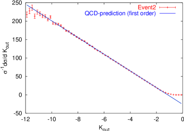
Figure 2: Comparison of fixed order QCD distribution with numerical simulations based on the exact four parton matrix element for $y_{3}>0.1$ in units of $(\alpha_{\mbox{\scriptsize s}}/(2\pi))^{2}$.

All effects of soft inter-jet gluon radiation and of hard parton collinear splitting are embodied in the scales $Q_{a}$, which depend on $T$ and $T_{M}$.

6 Conclusions and outlook

The most interesting feature of $K_{\mbox{\scriptsize out}}$ distribution in (13) is its geometry (i.e. $T$ and $T_{M}$) dependence, which allows to measure the effects of large angle gluon radiation.

In order to compare theory with experiments, one has to sum over all possible configurations and to integrate over $T$ and $T_{M}$ varying in an appropriate range. At this point some problems may arise.

Till now the available data explore all values of $T$ and $T_{M}$, but the dominant $T\!\sim\!1$ region has to be excluded for several reasons. First of all in this region our calculation is incomplete because the hard matrix element becomes IR singular as the emitting gluon becomes soft or collinear to the quark-antiquark pair, so that an additional resummation should be performed. Furthermore, in this region the definition of an event plane becomes problematic, if not even meaningless. Last but not least, even if we were able to perform the calculation, the result would not be interesting, since we lose the richness of three-jet event topology. In order to avoid this problem one should look for data in a “restricted” region, e.g. $T\!<\!0.9$. From an experimental point of view it is more convenient to put a cut in the three-jet resolution parameter. If one uses the Durham recombination algorithm [11], a suitable choice is, for example, $y_{3}>0.1$.

However, before any comparison with data may be attempted, some theoretical work has still to be made.

First of all one has to compare the resummed result with numerical NLO computation based on the exact two loop matrix element in order to check resummation to ${\cal{O}}\left(\alpha_{\mbox{\scriptsize s}}^{2}\ln^{2}\right)$ and to to compute the coefficient function $C(\alpha_{\mbox{\scriptsize s}})$ with the best achievable accuracy.

Then one has to match the resummed result with these fixed order calculations to obtain an improved prediction in the whole phase space considered.

But indeed the greatest effort shall be made to compute hadronization effects, the so-called non-perturbative (NP) “power-corrections”, which are due to the emission of gluons with $k_{t}\sim\Lambda_{\mbox{\scriptsize}QCD}$. We believe that these correction are of $1/Q$ type, enhanced by a factor $\ln K_{\mbox{\scriptsize out}}/Q$, in analogy with what happens for the jet Broadenings  [12]. This will be the aim of our research in the forthcoming period, and we hope that a complete (PT and NP) resummed $K_{\mbox{\scriptsize out}}$ distribution may appear soon.

Acknowledgements

We are grateful to Yuri Dokshitzer and Pino Marchesini, since without their aid this work would had never been possible, and to Gavin Salam for illuminating discussions and suggestions.

References

- [1] S. Catani, L. Trentadue, G. Turnock and B.R. Webber, Nucl. Phys. B 407 (1993) 3.
- [2] S. Catani and B.R. Webber, Phys. Lett. B 427 (1998) 377 [hep-ph/9801350].
-
[3]
S. Catani, G. Turnock and B.R. Webber,
Phys. Lett. B 295 (1992) 269;
Yu.L. Dokshitzer, A. Lucenti, G. Marchesini and G.P. Salam, JHEP 01 (1998) 011
[hep-ph/9801324]. -
[4]
M. Beneke,
Phys. Rep. 317 (1999) 1 [hep-ph/9807443];
B.R. Webber, Nucl. Phys. 71 (Proc. Suppl.) (1999) 66 [hep-ph/9712236]. Talk given at 27th International Symposium on Multiparticle Dynamics (ISMD 97), Frascati, Italy, 8-12 Sep 1997. - [5] Yu.L. Dokshitzer, Perturbative QCD and Power Corrections, Invited talk at 11th Rencontres de Blois: Frontiers of Matter, Chateau de Blois, France, 28 Jun – 3 Jul 1999 [hep-ph/9911299].
-
[6]
A. Banfi, Yu.L. Dokshitzer, G. Marchesini and
G. Zanderighi,
JHEP 07 (2000) 002
[hep-ph/0004027] - [7] S. Catani and M. Grazzini, [hep-ph/9908523]
- [8] Yu.L. Dokshitzer, A. Lucenti, G. Marchesini and G.P. Salam, Nucl. Phys. B 511 (1998) 396 [hep-ph/9707532].
- [9] S. Catani, G. Marchesini and B.R. Webber, Nucl. Phys. B 349 (1991) 635.
- [10] S. Catani and M.H. Seymour, Phys. Lett. B 378 (1996) 281, Acta Phys. Polon B 28 (1997) 863-881.
- [11] S. Catani, Yu.L. Dokshitzer, M. Olsson, G. Turnock and B.R. Webber, Phys. Lett. B 269 (1991) 233.
-
[12]
Yu.L. Dokshitzer, G. Marchesini and G.P. Salam,
Eur. Phys. J. Direct C 3 (1999) 1
[hep-ph/9812487].