QCD POTENTIOLOGY

We review the connection between QCD and potential models of quarkonia in the framework of effective field theories, with an emphasis on non-perturbative methods such as lattice simulations. The static and heavy quark potentials are introduced and the applicability of the non-relativistic and adiabatic approximations are discussed. The rôles of so-called hybrid potentials are explored and we comment on the QCD analogue of the QED Lamb shift.

1 Potential models

Long before direct non-perturbative QCD evaluations became feasible potential models, some QCD inspired and some not, turned out to be extremely useful for an understanding of the masses and decay rates of bottomonium ($\Upsilon$), charmonium ($J/\psi$) and $B_{c}$ states. The underlying idea is that when the quark mass $m$ is bigger than all other bound state energy scales, time scales $\Delta t_{Q}$ that characterise the relative heavy quark movement become much bigger than time scales $\Delta t_{g}$, associated with the gluon (and sea quark) dynamics, too. In this situation the leading Born-Oppenheimer (or adiabatic) approximation should be applicable and feedback effects of the moving heavy quarks onto the accompanying gluons and sea quarks might be neglected. If in addition the typical relative quark velocity is much smaller than the speed of light, $v=p/m\ll 1$, the bound state should be governed by a Schrödinger Hamiltonian,

$$H=2m+\frac{p^{2}}{2\mu_{R}}+V_{\mbox{\scriptsize phen}}(r),\quad H\psi_{n}=E_{n}\psi_{n},$$ (1)

where $\mu_{R}=m/2$ denotes the reduced mass and the potential $V_{\mbox{\scriptsize phen}}(r)$ parameterises the interaction that is mediated by gluons and sea quarks.

While in lattice QCD calculations spectrum and wave functions can in principle be predicted for a given set of quark masses and scale parameter, in the potential model approach one is initially confronted with the inverse problem of guessing or deriving the potential $V_{\mbox{\scriptsize phen}}$ from the knowledge of some energy levels and decay rates, before any predictions can be made. The experimental spin averaged quarkonia levels seem to constrain the potential (up to an additive constant) reasonably well for distances $0.2$ fm $<r<1$ fm to a form that can be represented in terms of a funnel (or Cornell) parametrisation, $\!{}^{{\bf?}}$

$$V_{\mbox{\scriptsize phen}}(r)=\sigma\,r-\frac{e}{r},$$ (2)

with $e\approx 0.5$ and a string tension $\sigma\approx 425^{2}\mbox{~{}MeV}^{2}$. The advantage of potential models over other approaches such as Lattice Gauge Theory or Spectral Sum Rules is the relative ease with which properties of radial excitations can be derived and the simplicity and transparency of the representation of the bound state problem in terms of a nonrelativistic quantum mechanical Hamiltonian.

If a potential model has anything to do with QCD, the heavy quark potential $V_{\mbox{\scriptsize phen}}(r)$ should be calculable on the lattice and such a determination should increase its predictive power. One object that is easily accessible in lattice studies is the so-called static potential, $V_{0}(r)$. In this article we shall address the following questions: does the “heavy quark potential” $V_{\mbox{\scriptsize phen}}$ exist? What is the relation between $V_{\mbox{\scriptsize phen}}$ and $V_{0}$? Can relativistic corrections systematically be incorporated into Eq. (1)?

2 QCD static potentials

Ironically, forgetting everything one knows about quarks and their properties like spin and mass seems to be a good strategy for an understanding of heavy quark bound state problems. After successfully mastering this first mental barrier one has to place an external colour charge $Q$ and anti-charge $Q^{*}$ at a distance $r$ into the QCD vacuum. The static potential $V_{0}(r)$ is then the energy difference of this configuration with respect to the vacuum energy. Since we are dealing with a quantum field theory, an additive mass renormalisation is required, due to the self energy of the point like sources,

$$V_{0,\mbox{\scriptsize phys}}(r)=V_{0}(\mu;r)-V_{\mbox{\scriptsize self}}(\mu),\quad V_{\mbox{\scriptsize self}}(\mu)\propto\mu/\ln\mu\quad(\mu\rightarrow\infty):$$ (3)

the static potential $V_{0}(\mu;r)$ diverges as the cut-off on gluon momenta $\mu$ is sent to infinity while, once a subtraction scheme is specified, $V_{0,\mbox{\scriptsize phys}}$ is well defined.

$V_{0}(\mu;r)$ can be computed from Wilson loops, for instance on a lattice with spacing $a\simeq\pi/\mu$. From perturbative QCD one would expect the generic Coulomb short distance form, $V_{0}(r)=-e/r$, where the effective $e=(4/3)\alpha_{R}(r)$ will logarithmically depend on the distance $r$ while — neglecting sea quarks — one might expect a linear rise at large distances, in agreement with the funnel parametrisation, Eq. (2).

In QCD the potential is the energy of a bound state of gluons and static sources. This contrasts the situation in QED where confinement is lacking and photons carrying any surplus energy will just be radiated away. In QCD a discrete spectrum of gluonic excitations exists, the so-called hybrid potentials, see e.g. $\!{}^{{\bf?},{\bf?}}$. This leads us to conclude that in addition to the distance $r$ another scale, $\Delta V(r)$, the gluonic binding energy, has to be considered. In a quenched setting $\Delta V(r=0)$ will be a glueball mass, the lightest of which is about 1.6 GeV, while in the case of QCD with sea quarks, radiation of a pair of pions becomes possible. While the coupling constant $\alpha_{s}(r^{-1})\rightarrow 0$ as $r\rightarrow 0$, $\alpha_{s}[\Delta V(r)]$ remains large at all distances, from which one might expect perturbation theory to break down when naïvely applied to the Wilson loop.

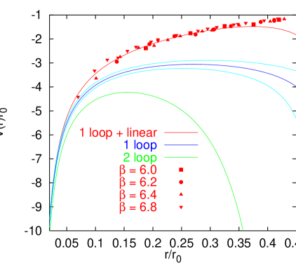
Figure 1: Comparison between the quenched lattice QCD potential (full symbols) and perturbation theory. $\!{}^{{\bf?},{\bf?}}$

In Fig. 1 we compare the quenched QCD potential, calculated on the lattice with continuum perturbation theory $\!{}^{{\bf?},{\bf?}}$ in units $r_{0}\approx 0.5$ fm at short distances, $r<0.23$ fm. Note that the $\Lambda$-parameter has been determined from an unrelated lattice observable, such that the only freedom in this representation is an additive constant, due to different values of $V_{\mbox{\scriptsize self}}$ in different regularisation schemes. Indeed, the perturbative series does not seem to convincingly approach the non-perturbative result and the coefficients of the perturbative expansion are large as indicated by the big difference between one- (order $\alpha_{s}^{2}$) and two-loop (order $\alpha_{s}^{3}$) potentials. This means that different resummation prescriptions will in general yield different two-loop results, some being closer to the non-perturbatively determined potential, some disagreeing even more.

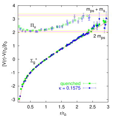
Figure 2: Static QCD potential and first hybrid excitation, without (quenched) and with ($\kappa=0.1575$) sea quarks. $\!{}^{{\bf?}}$

Gluonic excitations can be classified with respect to representations of the cylindrical symmetry group $D_{\infty h}$. The lowest hybrid excitation, in which the glue carries one unit of angular momentum about the intersource axis, is labelled by $\Pi_{u}$. A recent lattice result $\!{}^{{\bf?}}$ of both the static potential ($\Sigma_{g}^{+}$) and the hybrid potential $\Pi_{u}$, normalised such that $V_{0}(r_{0})=0$ is depicted in Fig. 2, both without sea quarks (quenched) and with 2 flavours of sea quarks, slightly lighter than the strange quark ($\kappa=0.1575$).

When including sea quarks the potential will eventually flatten around $\!{}^{{\bf?}}$ $r\approx 2.3\,r_{0}$ (string breaking) while in the quenched case the linear rise will continue. Within the region $r>0.2$ fm the lattice potentials can be fitted to the parametrisation Eq. (2), with the result $e\approx 0.3$ neglecting sea quarks and $e\approx 0.36$ with two flavours of light sea quarks.

3 The infra red problem of perturbation theory

In QED without fermions, the perturbative expansion of a Wilson loop can schematically be written as,

$$\langle W(r,\tau)\rangle=1+\mbox{\begin{minipage}{29.87547pt} \psfig{width=28.45274pt}\end{minipage}}+\frac{1}{2}\,\mbox{\begin{minipage}{29.87547pt} \psfig{width=28.45274pt}\end{minipage}}+\cdots=\exp\left(\mbox{\begin{minipage}{29.87547pt} \psfig{width=28.45274pt}\end{minipage}}\right):$$ (4)

multi-photon exchanges exponentiate! The solid lines denote the static sources and an integration of the vertices over all positions along the contour of the Wilson loop is understood to be included within the notation. The static potential in the limit of large Euclidean times $\tau$ is related to the Wilson loop,

$$\langle W(r,\tau)\rangle\propto\exp[-V_{0}(r)\tau]\qquad(\tau\rightarrow\infty),$$ (5)

which means that only contributions whose logarithms are proportional to $\tau$ have to be considered; interactions with the spatial closures of the loop can be ignored. The single photon exchange within the exponent on the right hand side of Eq. (4) can easily be calculated: a factor $\tau$ is obtained by translational invariance and the remaining time integral yields a $\delta$-function for the 4-component of the photon momentum. After a 3-dimensional Fourier transform one finds the well known result, $V_{0}=-\alpha_{\mbox{\scriptsize fs}}/r$ to all orders of perturbation theory.

The situation becomes somewhat more involved if fermions are included, due to the occurrence of diagrams such as,

$$D=\mbox{\begin{minipage}{44.10185pt} \psfig{width=42.67912pt}\end{minipage}}.$$ (6)

However, irreducible diagrams $D_{i}$ still exponentiate and the relation, $V_{0}(r)=-\lim_{\tau\rightarrow\infty}\sum_{i}dD_{i}(r,\tau)/d\tau$, holds. In a non-Abelian theory, starting from a two gluon exchange, the colour pre-factor of a given diagram depends on the ordering of the vertices along the contour of the Wilson loop. Hence, contributions are encountered that do not exponentiate anymore. $\!{}^{{\bf?}}$

Still, at least up to order $\alpha_{s}^{3}$, the static potential $V_{0}$ agrees with the result one obtains ignoring gluons that couple to the spatial closures of the Wilson loop, the so-called singlet potential $V_{s}$. Within perturbation theory it is also possible to define a so-called octet potential, $V_{o}$, by introducing colour generators at zero and infinite times into the colour traces. In doing so, one finds $V_{o}=-V_{s}/8$, at least to order $\alpha_{s}^{2}$. It is possible to calculate hybrid potentials in perturbation theory too, starting from linear combinations of Wilson loops where the spatial connections are deformed or colour fields are inserted. While for instance the hybrid potential $V_{\Pi_{u}}$ vanishes to order $\alpha_{s}$, the next excited state, $V_{\Sigma_{u}^{-}}$ agrees with $V_{o}$ to this order.

Up to order $\alpha_{s}^{3}$ non-Abelian contributions do not cause any fundamental problem, however, it has early been noticed $\!{}^{{\bf?}}$ that diagrams,

$$D_{\mbox{\scriptsize ADM}}=\mbox{\begin{minipage}{58.32823pt} \psfig{width=56.9055pt}\end{minipage}}\propto N^{2}C_{D}^{2}\alpha_{s}^{4}\tau\int_{0}^{\tau}\!\!\!\!dt\,\frac{1}{r^{2}+t^{2}}\frac{t}{r}\propto\alpha_{s}^{4}\tau\ln\tau,$$ (7)

diverge faster than $\tau$ as $\tau\rightarrow\infty$. This means that a naïve perturbative expansion of the static potential encounters an infra red problem: between the times $t_{1}$ and $t_{2}$ the quark and anti-quark are in a colour octet state and the first argument of the time integral should be proportional to $\exp(-\Delta Vt)$ with $\Delta V\simeq V_{o}-V_{s}$, which is small for times $t=t_{2}-t_{1}\gg\Delta V^{-1}$. However, in perturbation theory the real space propagator for large times only decays like $1/(r^{2}+t^{2})$ and this (wrong) behaviour finally causes the infra red divergence. It has therefore been suggested to regulate the encountered divergence by resumming all possible interactions $\!{}^{{\bf?}}$ between $t_{1}$ and $t_{2}$.

Since the infra red problem is related to the emission of an ultra-soft gluon, it has also been equated to the Lamb shift in the literature. $\!{}^{{\bf?}}$ One should, however, keep in mind that in QED the Lamb shift affects atomic bound states and not the Coulomb potential itself (which in QCD happens to be a bound state too). We shall see below that another “Lamb shift”, analogous to that of QED exists within quarkonia systems. One should also remember that while perturbation theory generically encounters problems when applied to bound states, the static potential is perfectly well defined in a non-perturbative context. Despite all problems with the static potential itself, Potential Nonrelativistic QCD $\!{}^{{\bf?}}$ (pNRQCD) might allow for a consistent and systematic perturbative treatment of heavy quark bound states. Within the pNRQCD Lagrangian a heavy quark singlet potential $V_{s}^{\mbox{\scriptsize pNRQCD}}$ appears that can be related to the static singlet potential $V_{s}$. It has been demonstrated $\!{}^{{\bf?}}$ that the divergence encountered in $V_{s}$ at order $\alpha_{s}^{4}$ is cancelled by a counter term from the matching of pNRQCD to QCD: the resulting $V_{s}^{\mbox{\scriptsize pNRQCD}}$ does not incorporate any singlet-octet-singlet transitions which are dealt with explicitely in the pNRQCD multipole expansion.

Finally, I mention the remarkable fact that up to order $\!{}^{{\bf?}}$ $\alpha_{s}^{3}$ potentials between charges within different representations $D$ of the gauge group scale in proportion to the respective Casimir factors, $C_{D}=(1/D)\mbox{tr}\,T_{a}^{D}T_{a}^{D}$. This Casimir scaling seems to be rather accurately satisfied in the non-perturbative regime too. $\!{}^{{\bf?}}$

4 The “heavy quark potential” from QCD

The natural starting point for deriving a non-relativistic Hamiltonian for quarkonia bound states is an effective field theory, NRQCD: $\!{}^{{\bf?},{\bf?}}$

$${\mathcal{L}}_{\mbox{\scriptsize NRQCD}}=-\psi^{\dagger}\left[m_{Q}+D_{4}-c_{2}\frac{{\mathbf{D}}^{2}}{2m_{Q}}+\cdots\right]\psi+\chi^{\dagger}\left[\cdots\right]\chi+{\mathcal{L}}_{\mbox{\scriptsize glue}}.$$ (8)

$\psi$ and $\chi$ are the quark and antiquark Pauli spinors. We eliminate the matching constant $c_{2}$ by defining $m=m_{Q}/c_{2}=m_{Q}+\delta m$, where $m_{Q}$ is the bare quark mass appearing in the original Dirac Lagrangian in Euclidean space, ${\mathcal{L}}=\bar{q}(D\!\!\!\!/+m_{Q})q$. The underlying idea of an effective field theory description is that if the quark mass is much bigger than exchange momenta and binding energy, QCD processes of scales $q\geq\mu>mv$ can be integrated out into local matching constants $c_{i}$.

For systems containing only one heavy quark the leading order effective Lagrangian will not incorporate the kinetic term and the usual heavy quark effective theory (HQET) power counting in powers of the inverse quark mass applies. However, heavyonia bound states cannot be addressed within a purely static theory, basically because, without a kinetic term, quarks that travel at different velocities will never interact with each other: hence, the leading order Lagrangian is that of Eq. (8). Since the static theory does not apply to quarkonia systems it is also not a priori clear whether the phenomenological potential $V_{\mbox{\scriptsize phen}}$ of Eq. (1) is at all related to the static potential $V_{0}$ in some approximation. $\!{}^{{\bf?}}$ To keep the discussion brief I will use the conventional power counting rules $\!{}^{{\bf?}}$ in the relative heavy quark velocity $v$ throughout this article. Several well founded objections to this scheme exist and other counting schemes have been suggested to be more suitable or better defined. $\!{}^{{\bf?},{\bf?},{\bf?},{\bf?},{\bf?}}$ According to the “standard” conventions the leading order NRQCD Lagrangian is counted as order $v^{2}$.

In Table 1 estimates of various scales for the charmonium, bottomonium and (unstable and, therefore, hypothetical) toponium ground states from a potential calculation $\!{}^{{\bf?}}$ are displayed. For comparison, we include the corresponding estimates for positronium. While binding energies and level splittings are of size $mv^{2}$ (ultra-soft), the momenta exchanged between the quarks are of order $mv$ (soft). NRQCD is the effective theory for physics at scales $q<\mu$, $mv\leq\mu\leq m$, while physics of scales $q>\mu$, has been integrated out into matching coefficients $c_{i}(m/\mu,\alpha_{s})$ that are in principle calculable from the QCD Lagrangian. It is possible to integrate out the soft scale $mv$ in a further step with the result of the effective theories, pNRQCD $\!{}^{{\bf?}}$ or vNRQCD. $\!{}^{{\bf?}}$

Table 1: Hard, soft and ultra-soft scale estimates. $\!{}^{{\bf?}}$

	$J/\psi$	$\Upsilon$	$t\bar{t}$	$e^{+}e^{-}$
$m$	1.4 GeV	4.7 GeV	175 GeV	511 keV
$mv$	0.7 GeV	1.3 GeV	45 GeV	3.7 keV
$mv^{2}$	0.4 GeV	0.4 GeV	12 GeV	0.027 keV
$v$	0.5	0.29	0.26	0.007

In NRQCD, being a nonrelativistic theory, the time evolution of a quark in a background gauge field, $\{A_{\mu}(x)\}$, is controlled by a Hamiltonian,

$$H_{\psi}=m-\delta m+igA_{4}-\frac{{\mathbf{D}}^{2}}{2m}+\cdots.$$ (9)

The quark propagator, $K=\psi\psi^{\dagger}$, obeys the evolution equation, $-d_{4}K=H_{\psi}K$, which for the initial condition, $\left.K(x,y)\right|_{x_{4}=y_{4}}=\delta^{3}({\mathbf{x}}-{\mathbf{y}})$, is solved by,

$$K(x,y)\propto\int_{{\mathbf{z}}(y_{4})={\mathbf{y}}}^{{\mathbf{z}}(x_{4})={\mathbf{x}}}\!\!\!\!\!D{\mathbf{z}}\,D{\mathbf{p}}\,\exp\left\{\int_{y_{4}}^{x_{4}}\!\!dt\,\left[{\mathbf{p}}\dot{{\mathbf{z}}}-H_{\psi}({\mathbf{z}},{\mathbf{p}})\right]\right\},$$ (10)

where the path integral is over all paths connecting $y$ with $x$.

For illustrative purposes we sketch the derivation of a quantum mechanical Hamiltonian for quarkonium systems to leading order in $v$: we combine two propagators for quark and antiquark into a four-point function,

$$G({\mathbf{r}},\tau;\cdots)=\mbox{\begin{minipage}{88.2037pt}\psfig{width=85.35826pt} \end{minipage}}=\frac{1}{3}\mbox{Re}\,\mbox{tr}\left\{U_{0}^{\dagger}K(y_{1},x_{1})U_{\tau}K(x_{2},y_{2})\right\}$$ (11)

$U_{\tau}$ denotes a gauge transporter at time $\tau$. To higher orders in the velocity expansion $G$ will not only depend on the distance but also on spin, angular momentum and momentum. It can be shown $\!{}^{{\bf?}}$ that to leading order only the shortest paths between $y_{i}$ and $x_{i}$ contribute to the path integral Eq. (10), such that after factorising the gauge field dependent and independent parts one obtains,

$$\langle G({\mathbf{r}},\tau)\rangle\propto\exp\left[-\int_{0}^{\tau}\!\!\!dt\,\sum_{j=1}^{2}\left(m_{j}-\delta m_{j}+\frac{{\mathbf{p}}_{j}^{2}}{2m_{j}}\right)\right]\langle W({\mathbf{r}},\tau)\rangle,$$ (12)

where $W({\mathbf{r}},\tau)$ is the usual Wilson loop and the expectation value is over gauge field configurations. Now the Hamiltonian $H$ that governs the evolution of the two-particle state, $H\langle G\rangle=-d_{4}\langle G\rangle$ can easily be read off,

$$H=2[m-\delta m(\mu)]+\frac{{\mathbf{p}}^{2}}{2\mu_{R}}+V_{0}(\mu;r),$$ (13)

where we have set $m=m_{1}=m_{2}=2\mu_{R}$. Indeed, the leading order Hamiltonian is that of Eq. (1) with $V_{\mbox{\scriptsize phen}}(r)=V_{0}(\mu;r)-2\delta m(\mu)$. The quantum mechanical Hamiltonian should not depend on the scale $\mu$. This implies the relation, $2\delta m(\mu^{\prime})=2\delta m(\mu)+V_{\mbox{\scriptsize self}}(\mu^{\prime})-V_{\mbox{\scriptsize self}}(\mu)$, between the mass shift $\delta m(\mu)$ between “kinetic” mass $m$ and QCD quark mass $m_{Q}(\mu)$ and the static self energy $V_{\mbox{\scriptsize self}}(\mu)$, defined in Eq. (3).

5 The “Lamb shift” and relativistic corrections

The assumption, $\Delta t_{g}>\Delta t_{Q}$, underlying the adiabatic approximation, is clearly violated whenever ultra-soft gluons with momenta smaller than the interaction energy are exchanged; at the end of an interaction time of order $\Delta t_{Q}$ such a gluon will still be present and cannot be integrated out into a potential. In the positronium case such effects result in the Lamb shift which can be accounted for by considering transitions between higher Fock states, $|e^{+}e^{-}\gamma\rangle,|e^{+}e^{-}\gamma\gamma\rangle,\ldots$ and $|e^{+}e^{-}\rangle$. Any formalism that does not incorporate such transitions can only be approximate. Where then is the loop hole of the derivation of Sec. 4 above? The definition of the 4-point Green function Eq. (11) is ambiguous since the $D_{\infty h}$ states of the gluonic connections $U_{0}$ and $U_{\tau}$ are unspecified. In general, $G$ will carry two more indices that run over gluonic excitations, $a,b=\Sigma_{g}^{+},\Pi_{u},\Sigma_{u}^{-},\cdots$, in addition to time, distance, spin, momentum and angular momentum of the quarks. The derivation of Eq. (13) can then be generalised, resulting in the Schrödinger equation $\!{}^{{\bf?}}$ $H_{ab}\psi^{b}_{n}=E\psi^{a}_{n}$, where the $J^{PC}$ quantum numbers of quarkonia eigenstates $\psi_{n}$ are products of quark and gluon quantum numbers. Physical states will be linear combinations of standard quark model states ($\Sigma_{g}^{+}$) and various hybrid excitations.

Table 2: Combinations of spins and angular momenta that can couple to $J^{PC}=1^{--}$.

$\Lambda^{\sigma_{v}}_{\eta}$	${\mathbf{\Sigma}_{g}^{+}}$	$\Sigma_{u}^{-}$	$\Pi_{u}$	$\Sigma_{g}^{-}$	$\Pi_{u}$	${\mathbf{\Sigma}_{g}^{+}}$	$\Pi_{u}$	$\Delta_{g}$
$K$	$S$	$P$	$P$	$P$	$P$	$D$	$D$	$D$
$S$	$1$	$0$	$0$	$1$	$1$	$1$	$1$	$1$

The off-diagonal elements $H_{\Sigma_{g}^{+}b}$ mediate transitions between standard states and states with excited glue and are related to gluon emission by the valence quarks. Each such element is accompanied by a pre-factor $gv$, $g=\sqrt{4\pi\alpha_{s}}$. We may therefore treat mixing effects as perturbations. Let us start from the unperturbed, diagonal Hamiltonian,

$$H_{aa}=2(m-\delta m)+\frac{{\mathbf{p}}_{a}^{2}}{2\mu_{R}}+V_{a}(r),\quad H_{aa}\psi_{n}^{0,a}=E_{n}^{0,a}\psi_{n}^{0,a}.$$ (14)

The energy shift of the state $n$ of the lowest lying channel ($a=\Sigma_{g}^{+}$) is,

$$\Delta E_{n}^{a}=\sum_{m,b\neq a}\frac{\left|\left\langle\psi_{n}^{0,a}\left|H_{ab}\right|\psi_{m}^{0,b}\right\rangle\right|}{E_{m}^{0,b}-E_{n}^{0,a}}={\mathcal{O}}\left(\alpha_{s}v^{2}E_{n}^{0,a}\right),$$ (15)

where only states with equal $J^{PC}$ content yield a non-vanishing matrix element in the nominator and $E_{n}=E_{n}^{0,\Sigma_{g}^{+}}+\Delta E_{n}^{\Sigma_{g}^{+}}+{\mathcal{O}}(v^{6})$. In Table 2 we have listed all possible combinations of gluonic $D_{\infty h}$ excitation $\Lambda^{\sigma_{v}}_{\eta}$, total angular momentum $K$ and spin $S$ of a vector particle ($J^{PC}=1^{--}$). It turns out that to order $v^{4}$ only mixing of the standard $S$ wave state with the $\Sigma_{u}^{-}$ $P$ wave state has to be considered. $\!{}^{{\bf?}}$ In this formalism spin exotic states like $1^{-+}$ that do not have any $\Sigma_{g}^{+}$ content are automatically accounted for.

Having understood these mixing effects, we can now say that “valence gluons” that accompany the quarks in the form of hybrid excitations of the flux tube and “sea gluons”, whose average effect can be integrated out into an interaction potential, can be distinguished from each other. To lowest order of the relativistic expansion pure quark model quarkonia and pure quark-gluon hybrids exist, which then undergo mixing with each other as higher orders in $v$ are incorporated. Moreover, at leading order the Hamiltonian is of Schrödinger type and $V_{\mbox{\scriptsize phen}}=V_{0}$. As soon as one allows for higher orders in the velocity expansion, an instantaneous interaction potential does not exist anymore but the corrections can systematically be accounted for.

With respect to QED the Lamb shift is naïvely enhanced by a relative factor, $\alpha_{s}v^{2}_{\Upsilon}/(\alpha_{\mbox{\scriptsize fs}}v^{2}_{e^{+}e^{-}})\approx 6\times 10^{4}$. However, below a certain glueball (or, when sea quarks are included, meson) radiation threshold, the spectrum of excitations is (unlike in the QCD case) discrete and the denominator of Eq. (15) will become large. It is clear that as long as gaps between hybrid potentials are bigger than quarkonia level splittings with respect to the $1S$ state, transitions will be energetically penalised: the wave function will only see the lowest lying potential and the adiabatic approximation is reliable while one might expect levels such as $\Upsilon(3S)$ and $\Upsilon(4S)$ to be affected by the presence of hybrid excitations.

We notice formal similarities between the discussion above and the pNRQCD Lagrangian that includes transition elements between two different states, singlet and octet. However, to draw the analogy, singlet $\simeq\Sigma_{g}^{+}$ and octet $\simeq$ hybrid, is not straight forward. Moreover, in the potential framework transitions between different $D_{\infty h}$ states are only possible via interactions between the valence quarks and the glue while in pNRQCD an ultra-soft gluon that causes a singlet-octet transition can also be radiated from another gluon. Effects of this latter kind are already included automatically in the non-perturbative matrix elements $H_{ab}$, defined through expectation values of Wilson loop like operators.

The velocity will approach zero only as a logarithmic function of the quark mass: the numbers of Table 1 reveal that $v^{2}$ is reduced from 0.085 to just 0.070 when replacing bottom quarks by (almost forty times heavier) top quarks. Therefore, although $v\rightarrow 0$ as $m\rightarrow\infty$, at any reasonable quark mass value one has to address Lamb shift effects as well as standard relativistic corrections which are also mandatory for an understanding of fine structure splittings.

The complete Hamiltonian to order $v^{4}$ is known $\!{}^{{\bf?},{\bf?},{\bf?},{\bf?},{\bf?},{\bf?}}$ where various corrections are given in terms of expectation values of Wilson loop like operators, most of which have been calculated on the lattice. $\!{}^{{\bf?},{\bf?}}$ In addition to Pauli, Thomas and Darwin like terms, momentum dependent corrections appear due to insertions of the operators $D_{4}$ and ${\mathbf{D}}^{2}/(2m)$ as well as $1/m$ and $1/m^{2}$ corrections that are spin- and momentum-independent. $\!{}^{{\bf?}}$ We remark that the momentum dependent corrections have nothing to do with the Lamb shift. The derivation can either be performed along the lines of Sec. 4 $\!{}^{{\bf?},{\bf?},{\bf?}}$ or in terms of quantum mechanical perturbations. $\!{}^{{\bf?},{\bf?},{\bf?}}$ The predictive power is at present in particular limited by an insufficient knowledge of the matching constants between QCD and NRQCD. For instance we estimate $\!{}^{{\bf?}}$ a related uncertainty of 25 % on $\Upsilon$ fine structure splittings while relativistic order $v^{6}$ corrections are unlikely to change order $v^{4}$ QCD potential predictions by more than 10 %.

6 Summary

We have demonstrated that in a non-relativistic situation, it is possible to factorise gluonic effects from the slower dynamics of the quarks and to derive “potential models” from QCD. Effective field theory methods turn out to be essential for this step. The resulting Hamiltonian representation of the bound state problem in terms of functions of canonical variables offers a very intuitive and transparent representation of quarkonium physics. It highlights parallels as well as differences to well understood atomic physics.

The adiabatic approximation is violated when ultra-soft gluons are radiated, i.e. when the nature of the bound state changes during the interaction time. Such effects can systematically be incorporated into the potential formulation by enlarging the basis of states onto which the Hamiltonian acts and a lattice study of the relevant transition matrix elements $H_{ab}$ is on its way. The validity of the adiabatic approximation is tied to that of the non-relativistic approximation in so far as off-diagonal entries of $H_{ab}$ are suppressed by powers of the velocity, $v$. Hybrid mesons become a well defined concept in the potential approach and translation into the variables used for instance in flux tube models is straight forward. In view of phenomenological applications, a precise determination of the matching coefficients between QCD and (lattice) NRQCD is required.

References

References

- [1] E. Eichten et al., Phys. Rev. Lett. 34, 369 (1975).
- [2] C. Michael, these proceedings [hep-ph/0009115].
- [3] G.S. Bali, Phys. Rep., in print [hep-ph/0001312].
- [4] G.S. Bali, Phys. Lett. B460, 170 (1999) [hep-ph/9905387].
- [5] G.S. Bali et al. [SESAM], Phys. Rev. D62, 054503 (2000) [hep-lat/0003012]; B. Bolder et al. [SESAM], Phys. Rev. D62, in print [hep-lat/0005018].
- [6] L. Susskind, in Weak and Electromagnetic Interactions at High Energy, ed. R. Balian and C. Llewellyn Smith (North Holland, Amsterdam, 1977); W. Fischler, Nucl. Phys. B129, 157 (1977).
- [7] T. Appelquist, M. Dine, I.J. Muzinich, Phys. Lett. B69, 231 (1977).
- [8] B.A. Thacker and G.P. Lepage, Phys. Rev. D43, 196 (1991).
- [9] N. Brambilla et al., Nucl. Phys. B566 (2000) 275 [hep-ph/9907240].
- [10] N. Brambilla et al., Phys. Rev. D60, 091502 (1999) [hep-ph/9903355].
- [11] Y. Schröder, Phys. Lett. B447, 321 (1999) [hep-ph/9812205] and private communication.
- [12] G.S. Bali, Phys. Rev. D62, in print [hep-lat/0006022].
- [13] W.E. Caswell and G.P. Lepage, Phys. Lett. B167, 437 (1986).
- [14] L.S. Brown and W.I. Weisberger, Phys. Rev. D20, 3239 (1979).
- [15] B. Grinstein, Int. J. Mod. Phys. A15, 461 (2000) [hep-ph/9811264].
- [16] M.E. Luke, A.V. Manohar, I.Z. Rothstein, Phys. Rev. D61, 074025 (2000) [hep-ph/9910209].
- [17] A. Vairo, these proceedings.
- [18] A. Barchielli, N. Brambilla, G.M. Prosperi, Nuovo Cim. A103, 59 (1990).
- [19] E. Eichten and F.L. Feinberg, Phys. Rev. Lett. 43, 1205 (1979).
- [20] G.S. Bali, K. Schilling, A. Wachter, Phys. Rev. D56, 2566 (1997) [hep-lat/9703019].
- [21] N. Brambilla, A. Pineda, J. Soto, A. Vairo, hep-ph/0002250; A. Pineda and A. Vairo, hep-ph/0009145.
- [22] G.S. Bali and P. Boyle, Phys. Rev. D59, 114504 (1999) [hep-lat/9809180].