Abstract
We show that the experimental data for the total virtual-photon proton cross section, $\sigma_{\gamma^{*}p}(W^{2},Q^{2})$, for $x_{bj}\mathrel{\hbox to0.0pt{\lower 4.0pt\hbox{\hskip 1.0pt$\sim$}\hss}\raise 1.0pt\hbox{$<$}}0.1$ lie on a universal curve, when plotted against $\eta=(Q^{2}+m^{2}_{0})/\Lambda^{2}(W^{2})$, where $\Lambda^{2}(W^{2})=C_{1}(W^{2}+W^{2}_{0})^{C_{2}}$ is determined by the parameters $C_{1},C_{2}$ and $W^{2}_{0}$. The observed scaling law follows from the generalized-vector-dominance/colour-dipole picture (GVD/CDP) of low-x deep inelastic scattering.

 

^∗ Supported by the BMBF, Bonn, Germany, Contract 05 HT9PBA2
^∗∗ On leave from BLTP JINR, Dubna, Russia

The present note will be concerned with deep inelastic scattering (DIS) in the kinematic range of low $x_{\rm bj}\simeq Q^{2}/W^{2}\ll 0.1$ that has been and is being explored at HERA. In particular, we will show that the data [1, 2, 3, 4, 5, 6] on photo- and electroproduction, for $x<0.1$, in good approximation, lie on a single curve, when plotted against the dimensionless (‘low-$x$ scaling’) variable

$$\eta=\frac{Q^{2}+m_{0}^{2}}{\Lambda^{2}(W^{2})}.$$ (1)

The value of the threshold mass, $m_{0}<m_{\rho^{0}}$, as well as the parameters $C_{1}$, $C_{2}$ and $W_{0}^{2}$ contained in

$$\Lambda^{2}(W^{2})=C_{1}(W^{2}+W_{0}^{2})^{C_{2}}$$ (2)

are fixed by the experimental data themselves.

We will proceed in two steps, the first one being a purely empirical analysis of the data, while in the second step, we will show, how the observed behaviour of $\sigma_{\gamma^{*}p}(W^{2},Q^{2})$ can be understood in terms of generalized vector dominance (GVD) [7, 8] or, equivalently [10], [11] the colour-dipole picture (CDP) [12].

1. In the first step, the model-independent phenomenological analysis of the experimental data, we assume the analytic form of the scaling variable $\eta$ according to (1) and (2), and, in addition, the existence of a continuous function of $\eta$ that is supposed to describe the data for $\sigma_{\gamma^{*}p}(W^{2},Q^{2})$, when these are plotted against $\eta$. For the technical analysis, we assume that this continuous function, without much loss of generality, may be represented by a piecewise linear function of $\eta$. This assumption allows us to perform a fit that determines the values of the parameters $m_{0}^{2}$, $C_{2}$ and $W_{0}^{2}$ simultaneously with the values of the piecewise linear function $\sigma_{\gamma^{*}p}(\eta)$ at a number of points, $\eta_{i}(i=1,...,N)$, of the variable $\eta$.

2. In the second step, we show how an approximate scaling law in terms of the variable $\eta$ follows from GVD or the CDP. We will restrict ourselves to only present the essential theoretical assumptions and conclusions. For a detailed account, we have to refer to a forthcoming paper [13].

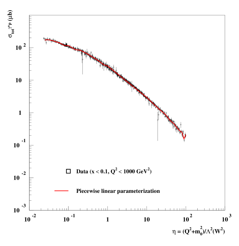
Figure 1: The experimental data for $\sigma_{\gamma^{*}p}(W^{2},Q^{2})$ for $x\simeq Q^{2}/W^{2}<0.1$ vs. the low-x scaling variable $\eta=(Q^{2}+m^{2}_{0})/\Lambda^{2}(W^{2})$.

Turning to step i), in fig.1, we show the result of the model-independent analysis. Imposing the kinematic restrictions of $x\leq 0.1$ and $Q^{2}\leq 1000\,$GeV², all available experimental data [1, 2, 3, 4, 5, 6] on photo- and electroproduction are indeed seen to lie on a smooth curve, that is approximated by the piecewise linear fit curve. The parameters that determine the scaling variable $\eta$ were found to be given by

$$m_{0}^{2} = 0.125\pm 0.0.027\;{\rm GeV^{2}},$$

$$C_{2} = 0.28\pm 0.06,$$

$$W_{0}^{2} = 439\pm 94\;{\rm GeV^{2}},$$ (3)

with a $\chi^{2}$ per degree of freedom ($ndf$) of $\chi^{2}/ndf=1.15$.

We add the remark, that an analogous procedure applied to the experimental data, without a restriction on $x$, does not lead to a universal curve. Likewise, restricting oneself to only those data points that belong to $x>0.1$, no universal curve is obtained either; the fitting procedure leads to entirely unacceptable results on the quality of the fit as quantified by the value of $\chi^{2}$ per degree of freedom.

We turn to step ii), the theoretical interpretation of the above results in terms of GVD or the CDP. Both pictures have in common the basic concept of virtual transitions of the photon to $q\bar{q}$ (or $q\bar{q}g$) vector states with subsequent diffractive scattering from the proton. Provided the configuration of the $q\bar{q}$ states the photon is coupled to, and the generic structure of two-gluon exchange [14] in the scattering from the proton is taken into account, (off-diagonal) GVD becomes identical [10] to the CDP. While GVD is conventionally formulated in terms of integrals over the masses of the propagating ($q\bar{q}$) vector states, and the two-dimensional momentum transfer (carried by the gluon), the CDP involves integration over the product of the square of the photon wave function and the ($q\bar{q}$)p (‘colour-dipole’) cross-section in transverse position space.

For the subsequent discussion, it will be useful, to note the relationship [10] between the colour-dipole cross-sections in (two-dimensional) transverse position space and in momentum-transfer space that guarantees the generic structure of two-gluon exchange,

$$\sigma_{(q\bar{q})p}(r^{2}_{\bot},z,W^{2})=\int d^{2}l_{\bot}\tilde{\sigma}_{(q\bar{q})p}(l^{2}_{\bot},z,W^{2})(1-\exp(-i\vec{l}_{\bot}\cdot\vec{r}_{\bot})).$$ (4)

Indeed from (4),

$$\sigma_{(q\bar{q})p}(r^{2}_{\bot},z,W^{2})\longrightarrow\cases{0,&for $r_{\bot}\rightarrow 0$,\cr\int d^{2}l_{\bot}\tilde{\sigma}_{(q\bar{q})p}(l^{2}_{\bot},z,W^{2}),&for $r_{\bot}\rightarrow\infty$,\cr}$$ (5)

thus fulfilling what has been called ‘colour transparency’ [12] and what indeed guarantees the generic structure of two-gluon exchange. This is explicitly seen [10], when representing $\sigma_{\gamma^{*}p}(W^{2},Q^{2})$ in momentum space. In connection with (4) and (5), we remind the reader of the notation being employed, the configuration of $q\bar{q}$ states being described by the (transverse) interquark separation, $r_{\bot}$, and the (light cone) variable, $z$, that is related to the $q\bar{q}$-rest-frame angle by $4z(1-z)\equiv\sin^{2}\theta$.

From (5), $\tilde{\sigma}_{(q\bar{q})p}(l^{2}_{\bot},z,W^{2})$ should vanish sufficiently rapidly to yield a convergent integral. Accordingly, it may be suggestive to assume a Gaussian in $l^{2}_{\bot}$ for $\tilde{\sigma}_{(q\bar{q})p}(l^{2}_{\bot},z,W^{2})$. Actually, explicit calculations become much simpler if, without much loss of generality, instead of a Gaussian a $\delta$-function located at a finite value of $l^{2}_{\bot}$ is used [10] as an effective description of $\tilde{\sigma}_{(q\bar{q})p}(l^{2}_{\bot},z,W^{2})$.

Accordingly, we will adopt the simple ansatz,

$$\tilde{\sigma}_{(q\bar{q})p}(l^{2}_{\bot},z,W^{2})=\sigma^{(\infty)}(W^{2})\frac{1}{\pi}\delta(l^{2}_{\bot}-z(1-z)\Lambda^{2}(W^{2})).$$ (6)

This ansatz associates with any given energy, $W$, an (effective) fixed value of (two-dimensional gluon) momentum transfer, $|\vec{l}_{\bot}|$, determined by the so far unspecified function $\Lambda(W^{2})$. The ansatz (6) also incorporates the assumption that ‘aligned’, $z\rightarrow 0$, configurations [15] of the $(q\bar{q})$ pair absorb vanishing, $l^{2}_{\bot}\rightarrow 0$, gluon momentum. For the subsequent interpretation of our results, we note the explicit form of the transverse-position-space colour-dipole cross section, obtained by substituting (6) into (4),

$$\sigma_{(q\bar{q})p}(r^{2}_{\bot},z,W^{2})=\sigma^{(\infty)}(W^{2})\left(1-J_{0}\left(r_{\bot}\cdot\sqrt{z(1-z)}\Lambda(W^{2})\right)\right)$$

$$\cong \sigma^{(\infty)}(W^{2})\cases{\frac{1}{4}z(1-z)\Lambda^{2}(W^{2})r^{2}_{\bot},&for $\frac{1}{4}z(1-z)\Lambda^{2}(W^{2})r^{2}_{\bot}\longrightarrow 0$,\cr&\cr 1&for $\frac{1}{4}z(1-z)\Lambda^{2}(W^{2})r^{2}_{\bot}\longrightarrow\infty$.\cr}$$

The limit of $\sigma^{(\infty)}(W^{2})$ in the second line of the approximate equality in (7) actually stands for an oscillating behaviour of the Bessel function, $J_{0}(r_{\bot}\sqrt{z(1-z)}\Lambda(W^{2}))$, around $\sigma^{(\infty)}(W^{2})$, when its argument tends towards infinity. Apart from these oscillations, the behaviour of $\sigma_{(q\bar{q})p}(r^{2}_{\bot},z,W^{2})$ in (7) is identical to the one obtained, if the $\delta$-function in (6) is replaced by a Gaussian. Concerning the high-energy behaviour of $\sigma_{(q\bar{q})p}(r^{2}_{\bot},z,W^{2})$, we note that it is consistent with unitarity restrictions, provided a decent high-energy behaviour is imposed on $\sigma^{(\infty)}(W^{2})$.

We stress that the ansatz (6) is by far not as specific as it might appear at first sight. It constitutes a simple effective realization, compare (7), of the underlying requirements of colour transparency, (4), (5), and hadronic unitarity for the colour-dipole cross section. The unitarity requirement enters via the decent high-energy behaviour of $\sigma^{(\infty)}(W^{2})$.

Referring to [13] for details, we note that the ansatz (6) allows one to simplify the GVD expression [10] for $\sigma_{\gamma^{*}p}(W^{2},Q^{2})$ (by integrating over $d^{2}l$ and $dz$) to become

$$\sigma_{\gamma^{*}p}(W^{2},Q^{2})=\sigma_{\gamma p}(W^{2})\frac{(I_{T}+I_{L})}{I_{T}|_{Q^{2}=0}},$$ (8)

where $\sigma_{\gamma p}(W^{2})$ denotes the photoproduction cross section, $\sigma_{\gamma^{*}p}(W^{2},Q^{2}=0)$, and the dimensionless quantities $I_{T}$ and $I_{L}$ contain integrations over the squares of the ingoing and outgoing masses, $M$ and $M^{{}^{\prime}}$, of the $q\bar{q}$ states coupled to the ingoing and outgoing photon in the (virtual) forward-Compton-scattering amplitude. Expression (8) contains the requirement of a smooth transition of $\sigma_{\gamma^{*}p}(W^{2},Q^{2})$ to photoproduction; it allowed us, to eliminate $\sigma^{(\infty)}(W^{2})$ in terms $\sigma_{\gamma p}(W^{2})$. Explicitly, the integrals $I_{T}$ and $I_{L}$, that are related to the transverse and longitudinal contributions to $\sigma_{\gamma^{*}p}(W^{2},Q^{2})$, respectively, are given by

$$I_{T}\left(\frac{Q^{2}}{\Lambda^{2}(W^{2})},\frac{m^{2}_{0}}{\Lambda^{2}(W^{2})}\right) ={1\over\pi}\int^{\infty}_{m^{2}_{0}}dM^{2}\int^{(M+\Lambda(W^{2}))^{2}}_{(M-\Lambda(W^{2}))^{2}}dM^{\prime 2}\omega(M^{2},M^{\prime 2},\Lambda^{2}(W^{2}))$$ (9)

$$\times\left[\frac{M^{2}}{(Q^{2}+M^{2})^{2}}-\frac{M^{\prime 2}+M^{2}-\Lambda^{2}(W^{2})}{2(Q^{2}+M^{2})(Q^{2}+M^{\prime 2})}\right],$$

and

$$I_{L}\left(\frac{Q^{2}}{\Lambda^{2}(W^{2})},\frac{m^{2}_{0}}{\Lambda^{2}(W^{2})}\right) ={1\over\pi}\int^{\infty}_{m^{2}_{0}}dM^{2}\int^{(M+\Lambda(W^{2}))^{2}}_{(M-\Lambda(W^{2}))^{2}}dM^{\prime 2}\omega(M^{2},M^{\prime 2},\Lambda^{2}(W^{2}))$$ (10)

$$\times\left[\frac{Q^{2}}{(Q^{2}+M^{2})^{2}}-\frac{Q^{2}}{(Q^{2}+M^{2})(Q^{2}+M^{\prime 2})}\right],$$

where the integration measure $\omega(M^{2},M^{\prime 2},\Lambda^{2}(W^{2}))$ fulfils

$$\frac{1}{\pi}\int^{(M+\Lambda(W^{2}))^{2}}_{(M-\Lambda(W^{2}))^{2}}dM^{\prime 2}\omega(M^{2},M^{\prime 2},\Lambda^{2}(W^{2}))=1.$$ (11)

The explicit expression for $\omega(M^{2},M^{\prime 2},\Lambda^{2}(W^{2})))$ is given in [10]. It is the form (8) to (10) of the theory that explicitly displays the structure [7, 8] of (off-diagonal) GVD. The appearance of $\Lambda(W^{2})$ in the integration limits over $dM^{{}^{\prime}2}$ is worth noting. One expects that the effective mass range for off-diagonal transitions, $M^{{}^{\prime}2}\neq M^{2}$, should increase with increasing energy, $W$, thus implying that $\Lambda(W^{2})$ should not be constant, but should increase with increasing energy.

We were able to derive explicit analytic expressions [13] for the integrals in (9) and (10). In the present context, we only note that, in very good approximation, the sum of $I_{T}$ and $I_{L}$ only depends on the dimensionless combination (1). While the general explicit expressions for $I_{T}$ and $I_{L}$ are complicated, in the most important limits, they become simple. Indeed,

$$I=I_{T}+I_{L}\equiv\cases{\log\left(\frac{\Lambda^{2}(W^{2})}{Q^{2}+m^{2}_{0}}\right),&for $\Lambda^{2}(W^{2})\gg Q^{2}+m^{2}_{0}$,\cr&\cr\frac{1}{2}\frac{\Lambda^{2}(W^{2})}{Q^{2}+m^{2}_{0}},&for $\Lambda^{2}(W^{2})\ll Q^{2}+m^{2}_{0}$.\cr}$$ (12)

In addition, $I_{L}$ vanishes for $Q^{2}$ towards zero.

As the moderate rise of photoproduction, $\sigma_{\gamma p}(W^{2})$, with energy, and the moderate logarithmic rise of the denominator in (8) approximately cancel each other, according to (12), we have indeed obtained approximate scaling of $\sigma_{\gamma^{*}p}(W^{2},Q^{2})$ in the variable $\eta$ defined in (1), i.e. $\sigma_{\gamma^{*}p}(W^{2},Q^{2})\simeq\sigma_{\gamma^{*}p}(\eta)$. Moreover, the theoretically expected increase of $\Lambda^{2}(W^{2})$ with increasing energy coincides with the above result, (3), of the phenomenological analysis of the experimental data.

The theoretical results (8) to (12) for $\sigma_{\gamma^{*}p}(W^{2},Q^{2})$ were obtained by incorporating the $q\bar{q}$ configuration in the virtual photon, as known from $e^{+}e^{-}$ annihilation, as well as the generic structure of two-gluon exchange into the ansatz for the virtual Compton-forward-scattering amplitude at low $x$. As stressed before, the simplifying $\delta$-function ansatz (6) is to be seen as an effective realization of the generic two-gluon exchange structure, combined with hadronic unitarity, without much loss of generality.

We turn to the analysis of the experimental data in terms of the theoretical results in (8) to (12). This essentially amounts to introducing an empirically satisfactory parameterization for the photoproduction cross-section, $\sigma_{\gamma p}(W^{2})$, and to determining the threshold mass, $m_{0}^{2}$, and the energy dependence of $\Lambda^{2}(W^{2})$ in fits to the experimental data.

Adopting a Regge parameterization for $\sigma_{\gamma p}(W^{2})$,

$$\sigma_{\gamma p}(W^{2})=A_{R}\cdot(W^{2})^{\alpha_{R}-1}+A_{P}\cdot(W^{2})^{\alpha_{P}-1},$$ (13)

where $W^{2}$ is to be inserted in units of GeV² and [16]

$$A_{R} = 145.0\pm 2.0\;{\rm\mu b},$$

$$\alpha_{R} = 0.5$$ (14)

$$A_{P} = 63.5\pm 0.9\;{\rm\mu b},$$

$$\alpha_{P} = 1.097\pm 0.002,$$

we again proceed in two steps.

In a first step, we do not impose any specific form for the functional dependence of $\Lambda^{2}(W^{2})$ except for the (technically necessary) assumption that $\Lambda^{2}(W^{2})$ can be represented by a piecewise linear function of $W^{2}$. A fit to the experimental data on $\sigma_{\gamma^{*}p}(W^{2},Q^{2})$ then determines the values of $\Lambda^{2}(W^{2}_{i})$, with $i=1,...,N$, that define the piecewise linear function, $\Lambda^{2}(W^{2})$. In fig.2, we show the result of this procedure, $\Lambda^{2}(W^{2}_{i})$ with $i=1,...,46$, including errors, obtained from the fit to the experimental data. For the fit, the restrictions of $x\leq 0.1$ and $Q^{2}\leq 100$ GeV² were applied to the data.

In a second step, we adopt the power-law ansatz (2), and again perform a fit to the data for $\sigma_{\gamma^{*}p}(W^{2},Q^{2})$. The agreement of the resulting curve for $\Lambda^{2}(W^{2})$ with the piecewise linear fit result in fig.2 shows that the power-law ansatz for $\Lambda^{2}(W^{2})$ is borne out by the data within the theoretical framework for $\sigma_{\gamma^{*}p}$ in (8) to (11), that specifies the $Q^{2}$ dependence. From the fit to the data under the restriction of $x\leq 0.01$ and $Q^{2}\leq 100$GeV², we obtained

$$m_{0}^{2} = 0.16\pm 0.01\;{\rm GeV^{2}},$$

$$C_{1} = 0.34\pm 0.05,$$ (15)

$$C_{2} = 0.27\pm 0.01,$$

$$W_{0}^{2} = 882\pm 246\;{\rm GeV^{2}},$$

with $\chi^{2}/ndf=1.15$.

The result (15), in particular the value of the exponent $C_{2}$ that determines the rise of $\Lambda^{2}(W^{2})$ with energy, is in reasonable agreement with the result (3) of the model-independent analysis. This implies that the $Q^{2}$ dependence of the data is correctly reproduced by the GVD/CDP in (8) to (12). In other words, our procedure that combines the model-independent analysis of the data with the one based on the GVD/CDP, has provided us with successful tests of the $W^{2}$- and $Q^{2}$-dependence that are independent from each other.

According to (7), the $W^{2}$ dependence of $\Lambda^{2}(W^{2})$, displayed in fig.2, determines the energy dependence of the colour-dipole cross section. The DIS experiments at low x directly measure this quantity, in particular for $Q^{2}\geq\Lambda^{2}(W^{2})$.

We have verified that the replacement of the power-law ansatz (2) for $\Lambda^{2}(W^{2})$ by a logarithmic one,

$$\Lambda^{2}(W^{2})=C_{1}^{\prime}\log(W^{2}/{W^{\prime}}^{2}_{0}+C_{2}^{\prime}),$$ (16)

leads to an equally good fit to the data. One finds

$$m_{0}^{2} = 0.157\pm 0.009\;{\rm GeV^{2}},$$

$$C_{1}^{\prime} = 1.64\pm 0.14,$$ (17)

$$C_{2}^{\prime} = 4.1\pm 0.4,$$

$${W^{\prime}}^{2}_{0} = 1015\pm 334\;{\rm GeV^{2}},$$

with $\chi^{2}/ndf=1.19$.

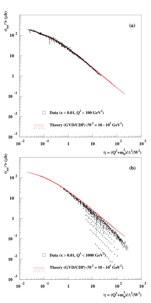
Figure 3: The GVD/CDP scaling curve for $\sigma_{\gamma^{*}p}$ compared with the experimental data a) for $x<0.01$, b) for $x>0.01$.

In fig.3, we show an explicit comparison of the experimental data with the GVD/CDP predictions. The (approximate) coincidence of the theoretical predictions for various values of $W^{2}$ demonstrates the scaling of the theory in terms of the low-x scaling variable $\eta$. Figure 3a, with the restrictions $x<0.01$ and $Q^{2}<100$ GeV² imposed on the data (as in the above fit) shows the good agreement between theory and experiment. In fig.3b, we show the deviations between theory and experiment, when the data for $x\geq 0.01$ are plotted

Finally, fig.4a demonstrates agreement of the GVD/CDP with experiment in a representation of $\sigma_{\gamma^{*}p}(W^{2},Q^{2})$ against $W^{2}$ for fixed values of $Q^{2}$. A subsample of all data used in the fit is presented for illustration.

The explicit analytical form of the theoretical expression for the cross-section, $\sigma_{\gamma^{*}p}(W^{2},Q^{2})$, allows us to investigate its behaviour at energies far beyond the ones being explored at HERA. According to (8) with (12), at any fixed $Q^{2}$, we have a strong power-like increase with energy, as $\Lambda^{2}(W^{2})$, while, finally, for sufficiently large energy, the power law turns into a logarithmic rise implying an energy behaviour as in photoproduction. This is explicitly seen in fig.4b. The approach to the asymptotic $W$ dependence becomes slower, if the power-law ansatz for $\Lambda^{2}(W^{2})$ in (2) is replaced by the logarithmic one in (16).

The transition from a strong power law (or ‘hard’) rise with energy to the soft rise in photoproduction is obviously related to the behaviour of the dipole cross-section (7) that in turn is largely dictated by the generic two-gluon exchange structure (4), (5) and the unitarity restriction on the growth of $\sigma^{(\infty)}(W^{2})$. At any (sufficiently small) fixed value of $r_{\bot}$, (corresponding to an approximately fixed value of $Q^{2}$), the dipole cross-section rises rapidly, as $\Lambda^{2}(W^{2})$, to finally settle down to the limiting value of $\sigma^{(\infty)}(W^{2})$, according to the second line on the right-hand side in (7). As seen in fig.4b, the scale for this transition to occur is extremely large, however, unless $Q^{2}$ is very small. It appears that even THERA energies of order $W^{2}\cong 10^{6}$ GeV² may be too small to see this transition in the energy dependence, except at sufficiently small $Q^{2}$.

The necessary extension of the present investigation to a careful treatment of charm and of the diffractively produced final states in general is beyond the scope of the present work.

The closest in spirit to the present investigation is the work by Forshaw, Kerley and Shaw [18] and by Golec-Biernat and Wüsthoff [19]. While we agree with the general picture of low-x DIS drawn by these authors, there are numerous essential differences though. In our treatment, the dependence of the colour-dipole cross section on the configuration variable $z$ is taken into account in contrast to refs.[18] and [19]. Our dipole cross section does not depend on $Q^{2}$, in agreement with the mass-dispersion relations (9), (10), but in distinction from the $Q^{2}$ (or rather $x$) dependence in ref.[19]. Decent high-energy behaviour at any $Q^{2}$ (“saturation”) follows from the underlying assumptions of colour transparency (the generic two-gluon exchange structure) and hadronic unitarity in distinction from the two-pomeron ansatz in ref.[18] and in ref.[22] that needs modification at energies beyond the ones explored at HERA.

In conclusion, a unique picture, the GVD/CDP, emerges for DIS in the low-x diffraction region. In terms of the (virtual) Compton-forward-scattering amplitude, the photon virtually dissociates into $(q\bar{q})$ vector states that propagate and undergo diffraction scattering from the proton as conjectured in GVD a long time ago. Our knowledge on the photon-$(q\bar{q})$ transition from $e^{+}e^{-}$ annihilation together with the gluon-exchange dynamics from QCD allows for a much more detailed theoretical description of $\sigma_{\gamma^{*}p}(W^{2},Q^{2})$ than available at the time when GVD was introduced. In terms of the GVD/CDP, experiments on DIS at low x measure the energy dependence of the $(q\bar{q})$/colour-dipole proton cross section, $\sigma_{(q\bar{q})p}(r^{2}_{\bot},z,W^{2})$. A strong energy dependence of this cross section for small interquark separation (not entirely unexpected within the GVD/CDP) is extracted from the data at large $Q^{2}$. The combination of colour transparency (generic two-gluon-exchange structure) with hadronic unitarity then implies that for any interquark separation the strong increase of the colour-dipole cross section, at sufficiently high energy, will settle down to the smooth increase of purely hadronic interactions. As a consequence, also the strong increase with energy of $\sigma_{\gamma^{*}p}(W^{2},Q^{2})$ at large $Q^{2}$ will eventually reach the behaviour observed in $(Q^{2}=0)$ photoproduction and hadron-hadron interactions.

Acknowledgement
One of us (D.S.) thanks the theory group of the Max-Planck-Institut für Physik in München, where part of this work was done, for warm hospitality. Thanks to Wolfgang Ochs for useful discussions, and particular thanks to Leo Stodolsky for his insistence that there should exist a simple scaling behaviour in DIS at low x. We thank G. Cvetic for useful discussions and collaboration during the early stages of this work, and we also thank John Dainton and A.B. Kaidalov for useful discussions at ‘Diffraction2000’ in Centraro (Sept. 2-7), where this work was first presented.

Figure 2: The dependence of $\Lambda^{2}$ on $W^{2}$, as determined by a fit of the GVD/CDP predictions for $\sigma_{\gamma^{*}p}$ to the experimental data.

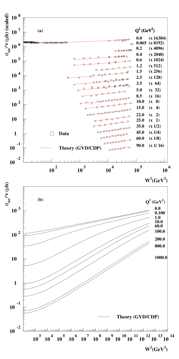
Figure 4: The GVD/CDP predictions for $\sigma_{\gamma^{*}p}(W^{2},Q^{2})$ vs. $W^{2}$ at fixed $Q^{2}$  a) in the presently accessible energy range compared with experimental data for $x\leq 0.01$,   b) for asymptotic energies. The cross-section results for $Q^{2}=0.0\ \mbox{GeV}^{2}$ refer to the total photoproduction measurements [6] and the extrapolated results at low $Q^{2}$ [16]. They were not explicitly included in the fit, but rather the Regge parameterization (13).

References

-
[1]
ZEUS 94: ZEUS Collab., M. Derrick et al., Z. f. Physik C72 (1996) 399.
ZEUS SVTX 95: ZEUS Collab., J. Breitweg et al., Eur. Phys. J. C7 (1999) 609.
ZEUS BPC 95: ZEUS Collab., J. Breitweg et al., Phys. Lett. B407 (1997) 432.
ZEUS BPT 97: ZEUS Collab., J. Breitweg et al., Phys. Lett. B487 (2000) 1-2, 53. -
[2]
H1 SVTX 95: H1 Collab., C. Adloff et al., Nucl. Phys. B497 (1997) 3.
H1 94: H1 Collab., S. Aid et al., Nucl. Phys. B470 (1996) 3. - [3] E665 Collab., Adams et al., Phys. Rev. D54 (1996) 3006.
- [4] NMC Collab., Arneodo et al., Nucl. Phys. B483 (1997) 3.
- [5] BCDMS Collab., Benvenuti et al., Phys. Lett. B223 (1989) 485.
-
[6]
ZEUS Collab., M. Derrick et al., Z. Phys. C63 (1994) 391;
H1 Collab., A. Aid et al., Z. Phys. C69 (1995) 27. -
[7]
J.J. Sakurai and D. Schildknecht, Phys. Lett.
40B (1972) 121;
B. Gorczyca and D. Schildknecht, Phys. Lett. 47B (1973) 71. -
[8]
H. Fraas, B.J. Read and D. Schildknecht, Nucl. Phys. B86
(1975) 346;
R. Devenish, D. Schildknecht, Phys. Rev. D19 (1976) 93. - [9] V.N. Gribov, Sov. Phys. JETP 30 (1970) 709.
-
[10]
G.Cvetic, D. Schildknecht, A. Shoshi, Eur. Phys. J. C 13, (2000) 301;
Acta Physica Polonica B30 (1999) 3265;
D. Schildknecht, Contribution to DIS2000 (Liverpool, April 2000), hep-ph/0006153. - [11] L. Frankfurt, V. Guzey, M. Strikman, Phys. Rev. D58 (1998) 094093.
- [12] N.N. Nikolaev, B.G. Zakharov, Z. Phys. C49, (1991) 607.
- [13] G. Cvetic, D. Schildknecht, B. Surrow, M. Tentyukov, in preparation.
- [14] J. Gunion, D. Soper, Phys. Rev. D15, (1977) 2617.
- [15] J.D. Bjorken, hep-ph/9601363
-
[16]
ZEUS Collab., J. Breitweg et al., Eur. Phys. J. C7
(1999) 609,
B. Surrow, Eur. Phys. J. direct C 2 (1999), 1. -
[17]
D. Schildknecht, G. Schuler and B. Surrow Phys. Lett. B 449
(1999) 328;
D. Schildknecht, Nucl. Phys. B (Proc. Suppl.) 79 (1999) 195. - [18] J. Forshaw, G. Kerley and G. Shaw, Phys. Rev. D60 (1999) 074012; hep-ph/0007257.
- [19] K. Golec-Biernat and M. Wüsthoff, Phys. Rev. D59 (1999) 014017; Phys. Rev. D60 (1999) 114023.
- [20] A.M. Stasto, K. Golec-Biernat and J. Kwiecinski, hep-ph 0007192.
- [21] M.F. McDermott, DESY00-126
- [22] A. Donnachie and P.V. Landshoff, Phys. Lett. B437 (1998) 408.