Can the SO(10) Model with Two Higgs Doublets
Reproduce the Observed Fermion Masses?

Abstract

It is usually considered that the SO(10) model with one 10 and one 126 Higgs scalars cannot reproduce the observed quark and charged lepton masses. Against this conventional conjecture, we find solutions of the parameters which can give the observed fermion mass spectra. The SO(10) model with one 10 and one 120 Higgs scalars is also discussed.

I Introduction

The grand unification theory (GUT) is very attractive as a unified description of the fundamental forces in the nature. Especially, the SO(10) model is the most attractive to us when we take the unification of the quarks and leptons into consideration. However, in order to reproduce the observed quark and lepton masses and mixings, usually, a lot of Higgs scalars are brought into the model. We think that the nature is simple. What is of the greatest interest to us is to know the minimum number of the Higgs scalars which can give the observed fermion mass spectra. A model with one Higgs scalar is obviously ruled out for the description of the realistic quark and lepton mass spectra. Then, how is a model with two different types of Higgs scalars (e.g., 10 and 126 scalars)?

In the SO(10) GUT scenario, a model with one 10 and one 126 Higgs scalars leads to the relation [1]

$$M_{e}=c_{u}M_{u}+c_{d}M_{d},$$ (1)

where $M_{e}$, $M_{u}$ and $M_{d}$ are charged lepton, up-quark and down-quark mass matrices, respectively. It is widely accepted that there will be almost no solution of $c_{u}$ and $c_{d}$ which give the observed fermion mass spectra. The reason is as follows: We take a basis on which the up-quark mass matrix $M_{u}$ is diagonal ($M_{u}=D_{u}$). Then, the relation (1) is expressed as

$$\widetilde{M_{e}}=c_{u}D_{u}+c_{d}\widetilde{M_{d}}.$$ (2)

Considering that $\widetilde{M_{d}}$ is almost diagonal and the mass hierarchy of up-quark sector is much severe than that of down-quark sector, we observe that the contribution to the first and the second generation part of $\widetilde{M_{e}}$ from the up-quark part $D_{u}$ is negligible so that it is proportional to that of $\widetilde{M_{d}}$. Thus, the relation (1) which predicts $m_{e}/m_{\mu}{\simeq}m_{d}/m_{s}$ does not reproduce the observed hierarchical structure of the down-quark and charged lepton masses [2] such as predicted by Georgi-Jarlskog mass relations $m_{b}=m_{\tau}$, $m_{s}=m_{\mu}/3$ and $m_{d}=3m_{e}$ at the GUT scale [3]. However, the above conclusion is somewhat impatient one. (i) It is too simplified to regard $\widetilde{M_{d}}$ as almost diagonal. (ii) We must check a possibility that the mass relations are satisfied with the opposite signs, i.e., $m_{b}={\pm}m_{\tau}$, $m_{s}={\pm}m_{\mu}/3$ and $m_{d}={\pm}3m_{e}$. (iii) The mass values at the GUT scale which are evaluated from the observed values by using the renormalization group equations show sizable deviations from the Georgi-Jarskog relations. The purpose of the present paper is to investigate systematically whether there are solutions of $c_{u}$ and $c_{d}$ which give the realistic quark and lepton masses or not.

II Outline of the investigation

In the SO(10) GUT model with one 10 and one 126 Higgs scalars, the down-quark and down-lepton mass matrices $M_{d}$ and $M_{e}$ are given by

$$M_{d}=M_{0}+M_{1},\ \ M_{e}=M_{0}-3M_{1},$$ (3)

where $M_{0}$ and $M_{1}$ are mass matrices which are generated by the 10 and 126 Higgs scalars $\phi_{10}$ and $\phi_{126}$, respectively. Inversely, we obtain

$$M_{0}={\frac{1}{4}}(3M_{d}+M_{e}),\ \ M_{1}={\frac{1}{4}}(M_{d}-M_{e}).$$ (4)

On the other hand, the up-quark mass matrix $M_{u}$ is given by

$$M_{u}=c_{0}M_{0}+c_{1}M_{1},$$ (5)

where

$$c_{0} = v_{0}^{u}/v_{0}^{d}=\langle\phi^{u0}_{10}\rangle/\langle\phi^{d0}_{10}\rangle,$$ (6)

$$c_{1} = v_{1}^{u}/v_{1}^{d}=\langle\phi^{u0}_{126}\rangle/\langle\phi^{d0}_{126}\rangle,$$ (7)

and $\phi^{u}$ and $\phi^{d}$ denote Higgs scalar components which couple with up- and down-quark sectors, respectively. Therefore, by using the relations Eq.(4), we obtain the relation

$$M_{e}=c_{d}M_{d}+c_{u}M_{u},$$ (8)

where

$$c_{d}=-{\frac{3c_{0}+c_{1}}{c_{0}-c_{1}}}\ ,\ \ c_{u}={\frac{4}{c_{0}-c_{1}}}\ .$$ (9)

For convenience, first, we investigate the case that the matrices $M_{u}$, $M_{d}$ and $M_{e}$ are symmetrical matrices at the unification scale because we assume that they are generated by the 10 and 126 Higgs. Then, we can diagonalize those by unitary matrices $U_{u}$, $U_{d}$ and $U_{e}$, respectively, as

$$U_{u}^{T}M_{u}U_{u}=D_{u}\ ,\ \ U_{d}^{T}M_{d}U_{d}=D_{d}\ ,\ U_{e}^{T}M_{e}U_{e}=D_{e}\ ,$$ (10)

where $D_{u}$, $D_{d}$ and $D_{e}$ are diagonal matrices. Since the Cabibbo-Kobayashi-Maskawa (CKM) matrix $V$ is given by

$$V=U_{u}^{T}U_{d}^{*}\ ,$$ (11)

the relation (8) is re-written as follows:

$$(U_{e}^{\dagger}U_{u})^{T}D_{e}(U_{e}^{\dagger}U_{u})=c_{d}VD_{d}V^{T}+c_{u}D_{u}.$$ (12)

At present, we have almost known the experimental values of $D_{e}$, $D_{u}$ and $VD_{d}V^{\dagger}$. Therefore, we obtain the independent three equations:

  

$${\rm Tr}D_{e}D_{e}^{\dagger} = |c_{d}|^{2}\,{\rm Tr}\Bigl{[}(VD_{d}V^{T}+\kappa D_{u})(VD_{d}V^{T}+\kappa D_{u})^{\dagger}\Bigr{]},$$ (13)

$${\rm Tr}(D_{e}D_{e}^{\dagger})^{2} = |c_{d}|^{4}\,{\rm Tr}\Bigl{[}((VD_{d}V^{T}+\kappa D_{u})(VD_{d}V^{T}+\kappa D_{u})^{\dagger})^{2}\Bigr{]},$$ (14)

$${\rm det}D_{e}D_{e}^{\dagger} = |c_{d}|^{6}\,{\rm det}\Bigl{[}(VD_{d}V^{T}+\kappa D_{u})(VD_{d}V^{T}+\kappa D_{u})^{\dagger}\Bigr{]},$$ (15)

  

where $\kappa=c_{u}/c_{d}$. By eliminating the parameter $c_{d}$, we have two equations for the parameter $\kappa$:

$$\frac{(m_{e}^{2}+m_{\mu}^{2}+m_{\tau}^{2})^{3}}{m_{e}^{2}m_{\mu}^{2}m_{\tau}^{2}} = \frac{(\ref{eq82501})^{3}}{(\ref{eq82503})},$$ (16)

$$\frac{(m_{e}^{2}+m_{\mu}^{2}+m_{\tau}^{2})^{2}}{2(m_{e}^{2}m_{\mu}^{2}+m_{\mu}^{2}m_{\tau}^{2}+m_{\tau}^{2}m_{e}^{2})} = \frac{(\ref{eq82501})^{2}}{(\ref{eq82501})^{2}-(\ref{eq82502})},$$ (17)

where $(\ref{eq82501})^{3}$, for instance, means the right-hand side of (13) to the third power. Let us denote the parameter values of $\kappa$ evaluated from (16) and (17) as ${\kappa}_{A}$ and ${\kappa}_{B}$, respectively. If ${\kappa}_{A}$ and ${\kappa}_{B}$ coincide with each other, then we have a possibility that the SO(10) GUT model can reproduce the observed quark and lepton mass spectra. If ${\kappa}_{A}$ and ${\kappa}_{B}$ do not so, the SO(10) model with one 10 and one 126 Higgs scalars is ruled out, and we must bring more Higgs scalars into the model. Of course, in the numerical evaluation, the values ${\kappa}_{A}$ and ${\kappa}_{B}$ will have sizable errors, because the observed values $D_{e}$, $D_{u}$, $D_{d}$ and $V$ have experimental errors, and the values at the GUT scale also have errors. The values $\kappa_{A}$ and $\kappa_{B}$ are not so sensitive to the renormalization group equation effect (evolution effect), because those are almost determined only by the mass ratios. (More details will be discussed in the Sec. III.) Therefore, we will evaluate ${\kappa}_{A}$ and ${\kappa}_{B}$ by using the center values at $\mu=m_{Z}$ in the Sec. IV. If we find $\kappa_{A}\simeq\kappa_{B}$, we will give further detailed numerical study only for the case.

III Evolution effect

The relations (2.13) and (2.14) hold only at the unification scale $\mu=\Lambda_{X}$ On the other hand, we know only the experimental values of the fermion masses $m_{f}$ and CKM matrix parameters $V_{ij}$ at the electroweak scale $\mu=m_{Z}$. For a model which does not have any intermediate energy scales, we can straightforwardly estimate the values of $m_{f}$ and $V_{ij}$ at $\mu=\Lambda_{X}$ from those at $\mu=m_{Z}$ by the one-loop renormalization equation

$$\frac{dY_{f}}{dt}=\frac{1}{16\pi^{2}}(T_{f}-G_{f}+H_{f})Y_{f}$$ (18)

where $T_{f}$, $G_{f}$ and $H_{f}$ denote contributions from fermion-loop corrections, vertex corrections due to the gauge bosons and vertex corrections due to the Higgs boson(s), respectively. Therefore, we can directly check the relations (2.13) and (2.14) by substituting the observable quantities $m_{f}$ and $V_{ij}$ at $\mu=\Lambda_{X}$. However, for a model which has an intermediate energy scale such as a non-SUSY model, the values of $m_{f}$ and $V_{ij}$ at $\mu=\Lambda_{X}$ are highly model-dependent, so that the check of Eqs. (2.13) and (2.14) cannot be done so straightforwardly.

In this section, we will show that we can approximately check Eq. (2.13) and (2.14) by using the values of $m_{f}$ and $V_{ij}$ at $\mu=m_{Z}$, without knowing the explicit values of $m_{f}$ and $V_{ij}$ at $\mu=\Lambda_{X}$, as far as the evolutions of $m_{f}$ and $V_{ij}$ are not singular.

It is well known that in such a conventional model the evolution effects are approximately described as [4]

$$\frac{m_{u}^{0}/m_{t}^{0}}{m_{u}/m_{t}}\simeq\frac{m_{c}^{0}/m_{t}^{0}}{m_{c}/m_{t}}\simeq 1+\varepsilon_{u}\ ,$$ (19)

$$\frac{m_{d}^{0}/m_{b}^{0}}{m_{d}/m_{b}}\simeq\frac{m_{s}^{0}/m_{b}^{0}}{m_{s}/m_{b}}\simeq 1+\varepsilon_{d}\ ,$$ (20)

$$\frac{|V_{ub}^{0}|}{|V_{ub}|}\simeq\frac{|V_{cb}^{0}|}{|V_{cb}|}\simeq\frac{|V_{td}^{0}|}{|V_{td}|}\simeq\frac{|V_{ts}^{0}|}{|V_{ts}|}\simeq 1+\varepsilon_{d}\ ,$$ (21)

$$\frac{m_{u}^{0}/m_{c}^{0}}{m_{u}/m_{c}}\simeq\frac{m_{d}^{0}/m_{s}^{0}}{m_{d}/m_{s}}\simeq\frac{|V_{us}^{0}|}{|V_{us}|}\simeq\frac{|V_{cd}^{0}|}{|V_{cd}|}\simeq 1\ ,$$ (22)

where $m_{q}^{0}$ and $V_{ij}^{0}$ ($m_{q}$ and $V_{ij}$) denote the values at $\mu=\Lambda_{X}$ ($\mu=m_{Z}$). The relations (3.2) hold only for a model where the Yukawa coupling constant of top quark, $y_{t}\equiv(Y_{u})_{33}$, satisfies $y_{t}\gg(Y_{d})_{ij}$ ($i,j=1,2,3$). The relations (3.2) also hold even in a model which has an intermediate energy scale $\Lambda_{I}$, because, for example, when we denote $(m_{u}/m_{t})_{\mu=\Lambda_{X}}/(m_{u}/m_{t})_{\mu=\Lambda_{I}}$ and $(m_{u}/m_{t})_{\mu=\Lambda_{I}}/(m_{u}/m_{t})_{\mu=m_{Z}}$ as $1+$$\varepsilon_{u1}$ and $1+$$\varepsilon_{u2}$, respectively, we can obtain $(m_{u}/m_{t})_{\mu=\Lambda_{X}}/(m_{u}/m_{t})_{\mu=m_{Z}}\simeq 1+\varepsilon_{u}$ with $\varepsilon_{u}=\varepsilon_{u1}+\varepsilon_{u2}$.

By using the approximate relations (3.2) the diagonalized up-quark mass matrix $D_{u}^{0}$ at $\mu=\Lambda_{X}$ is presented as

$$D_{u}^{0} = m_{t}^{0}\left(\begin{array}[]{ccc}m_{u}^{0}/m_{t}^{0}&0&0\\ 0&m_{c}^{0}/m_{t}^{0}&0\\ 0&0&1\end{array}\right)$$ (26)

$$\simeq m_{t}^{0}\left(\begin{array}[]{ccc}m_{u}/m_{t}&0&0\\ 0&m_{c}/m_{t}&0\\ 0&0&1\end{array}\right)\left(\begin{array}[]{ccc}1+\varepsilon_{u}&0&0\\ 0&1+\varepsilon_{u}&0\\ 0&0&1\end{array}\right)$$ (33)

$$= \frac{m_{t}^{0}}{m_{t}}(1+\varepsilon_{u}S)D_{u},$$ (34)

where

$$S=\left(\begin{array}[]{ccc}1&0&0\\ 0&1&0\\ 0&0&0\end{array}\right)\ .$$ (35)

Similarly, the matrix $D_{d}^{0}$ is given by

$$D_{d}^{0}\simeq\frac{m_{b}^{0}}{m_{b}}(1+\varepsilon_{d}S)D_{d}.$$ (36)

The CKM matrix $V^{0}$ at $\mu=\Lambda_{X}$ is given by

$$V^{0} \simeq \left(\begin{array}[]{ccc}1&V_{us}&V_{ub}(1+\varepsilon_{d})\\ V_{cd}&1&V_{cb}(1+\varepsilon_{d})\\ V_{td}(1+\varepsilon_{d})&V_{ts}(1+\varepsilon_{d})&1\end{array}\right)$$ (40)

$$\simeq ({\bf 1}+\varepsilon_{d}S_{3})V({\bf 1}+\varepsilon_{d}S_{3})-2\varepsilon_{d}S_{3}\ ,$$ (41)

where $S_{3}={\bf 1}-S$ and ${\bf 1}$ is a $3\times 3$ unit matrix. By using the relations (3.4) - (3.6), we can obtain the approximate expression

$$V^{0}D_{d}^{0}V^{0T}\simeq\frac{m_{b}^{0}}{m_{b}}\left[(1+\varepsilon_{d})VD_{d}V^{T}-\varepsilon_{d}m_{b}S_{3}\right],$$ (42)

where we have used the observed hierarchical relations among the quark mass ratios and CKM matrix parameters. Therefore, the matrix $VD_{d}V^{T}+\kappa D_{u}$ in Eqs. (2.10)-(2.12) is given by

$$K^{0} \equiv V^{0}D_{d}^{0}V^{0T}+\kappa^{0}D_{u}^{0}$$ (43)

$$\simeq (1+\varepsilon_{d})\frac{m_{b}^{0}}{m_{b}}\left(VD_{d}V^{T}+\kappa D_{u}\right.$$ (45)

$$\left.-\varepsilon_{d}m_{b}S_{3}+\varepsilon_{u}\kappa D_{u}S\right)\ ,$$

where

$$\kappa=\frac{m_{t}^{0}/m_{t}}{m_{b}^{0}/m_{b}}\frac{\kappa^{0}}{1+\varepsilon_{d}}\ .$$ (46)

Since the solutions $\kappa$ are of the order of $10^{-2}$ as we show in the next section, we can neglect the term $\kappa D_{u}S$ compared with $VD_{d}V^{T}$ (note that in order to neglect the component $(D_{u}S)_{11}$ it is essential that the sign of $m_{d}/m_{s}$ is positive, because $(VD_{d}V^{T})_{11}\simeq m_{d}+V_{us}^{2}m_{s}$ and $V_{us}^{2}\simeq|m_{d}/m_{s}|$). On the other hand, for such a small value of $\kappa$, the term $m_{b}S_{3}$ cannot be neglected compared with the term $\kappa D_{u}$. However, for a small value of $\varepsilon_{d}$, we can find that the solutions $\kappa$ are substantially not affected by the term $\varepsilon_{d}m_{b}S_{3}$. As a result, we obtain the approximate expression

$$K^{0}\simeq(1+\varepsilon_{d})\frac{m_{b}^{0}}{m_{b}}\left(VD_{d}V^{T}+\kappa D_{u}\right).$$ (47)

Therefore, Eq. (2.13) and (2.14) at $\mu=\Lambda_{X}$, i.e.,

$$\frac{[(m_{e}^{0})^{2}+(m_{\mu}^{0})^{2}+(m_{\tau}^{0})^{2}]^{3}}{(m_{e}^{0})^{2}(m_{\mu}^{0})^{2}(m_{\tau}^{2})^{2}}=\frac{[{\rm Tr}(K^{0}K^{0\dagger}])]^{3}}{{\rm det}(K^{0}K^{0\dagger})}\ ,$$ (48)

$$\frac{[(m_{e}^{0})^{2}+(m_{\mu}^{0})^{2}+(m_{\tau}^{0})^{2}]^{2}}{2[(m_{e}^{0})^{2}(m_{\mu}^{0})^{2}+(m_{\mu}^{0})^{2}(m_{\tau}^{0})^{2}+(m_{\tau}^{0})^{2}(m_{e}^{0})^{2}]}$$ (49)

$$=\frac{[{\rm Tr}(K^{0}K^{0\dagger})]^{2}}{[{\rm Tr}(K^{0}K^{0\dagger})]^{2}-{\rm Tr}(K^{0}K^{0\dagger})^{2}}\ ,$$ (50)

are approximately replaced by the relations at $\mu=m_{Z}$:

$$\frac{(m_{e}^{2}+m_{\mu}^{2}+m_{\tau}^{2})^{3}}{m_{e}^{2}m_{\mu}^{2}m_{\tau}^{2}}=\frac{[{\rm Tr}(KK^{\dagger})]^{3}}{{\rm det}(KK^{\dagger})}\ ,$$ (51)

$$\frac{(m_{e}^{2}+m_{\mu}^{2}+m_{\tau}^{2})^{2}}{2(m_{e}^{2}m_{\mu}^{2}+m_{\mu}^{2}m_{\tau}^{2}+m_{\tau}^{2}m_{e}^{2})}$$ (52)

$$=\frac{[{\rm Tr}(KK^{\dagger})]^{2}}{{\rm Tr}[(KK^{\dagger})]^{2}-{\rm Tr}(KK^{\dagger})^{2}}\ ,$$ (53)

where

$$K=VD_{d}V^{\dagger}+\kappa D_{u}\ ,$$ (54)

and $\kappa$ is given by Eq. (3.9). This means that when we find the solution $\kappa$ at $\mu=m_{Z}$, the solution at $\mu=\Lambda_{X}$ also exists, no matter whether the model is a SUSY one or a non-SUSY one. Then, we can obtain the value $\kappa^{0}$ at $\mu=\Lambda_{X}$ from the relation (3.9) with the solution $\kappa$ at $\mu=m_{Z}$.

IV Numerical study at $\mu=m_{Z}$

As mentioned in the preceding section, if the solution $\kappa$ exists at the energy scale $\mu=m_{Z}$, the one at $\mu=\Lambda_{X}$ also exists. Therefore, we investigate the relations (2.13) and (2.14) at $\mu=m_{Z}$. Note that Eqs.(16) and (17) are realized by GUT scale because Eq.(10) is broken at $\mu=m_{Z}$. In the present section, tentatively, we assume that the Yukawa coupling constant $Y_{10}$ and $Y_{126}$ at $\mu=m_{Z}$ keep their forms symmetrical, so that we can put the observed values $D_{u}$, $D_{d}$ and $V$ at $\mu=m_{Z}$ into the relations (16) and (17). For the fermion masses at $\mu=m_{Z}$, we use the following values: [5]

$$m_{t}=181\pm 13\ {\rm GeV},\hskip 25.6073ptm_{b}=3.00\pm 0.11\ {\rm GeV},$$ (55)

$$m_{c}=677^{+56}_{-61}\ {\rm MeV},\hskip 31.2982ptm_{s}=93.4^{+11.8}_{-13.0}\ {\rm MeV},$$ (56)

$$m_{u}=2.33^{+0.42}_{-0.45}\ {\rm MeV},\hskip 19.91684ptm_{d}=4.69^{+0.60}_{-0.66}\ {\rm MeV},$$ (57)

$$m_{\tau}=1746.7\pm 0.3\ {\rm MeV},$$ (58)

$$m_{\mu}=102.75138\pm 0.00033\ {\rm MeV},$$ (59)

$$m_{e}=0.48684727\pm 0.00000014\ {\rm MeV}.$$ (60)

The input values for the CKM matrix parameters have been taken as [6]

$$\theta_{12} = 0.219-0.226,\hskip 14.22636pt\theta_{23}=0.037-0.043,$$ (61)

$$\theta_{13} = 0.002-0.005,$$ (62)

where

  

$$V=\left(\begin{array}[]{ccc}c_{13}c_{12}&c_{13}s_{12}&s_{13}e^{-i\delta}\\ -c_{23}s_{12}-s_{23}c_{12}s_{13}e^{i\delta}&c_{23}c_{12}-s_{23}s_{12}s_{13}e^{i\delta}&s_{23}c_{13}\\ s_{23}s_{12}-c_{23}c_{12}s_{13}e^{i\delta}&-s_{23}c_{12}-c_{23}s_{12}s_{12}s_{13}e^{i\delta}&c_{23}c_{13}\end{array}\right),$$ (63)

  

with $c_{ij}\equiv\cos\theta_{ij}$ and $s_{ij}\equiv\sin\theta_{ij}$. The calculation has been performed allowing all the combinations of the quark mass signatures. Here it should be noted that, since $m_{u}$ is much smaller than $m_{c}$ and $m_{t}$, the difference of the sign of $m_{u}$ scarcely makes a change of allowed regions. In this calculation, we have selected $\theta_{23}$ and $\delta$ as input parameters and $m_{s}$, $c_{d}$ and $\kappa$ as output parameters because the calculation is sensitive to these parameters. We give the numerical results in Fig 1. Here, except for $m_{s}$, $\theta_{23}$ and $\delta$, we have adopted the center values of Eq.(57) as input values. Moving $\theta_{23}$ at intervals of 0.0005 rad and fixing $\delta=60{\rm{}^{\circ}}$, we search the solutions where $\kappa_{A}$ and $\kappa_{B}$ become coincident. Our numerical analysis shows that the solutions exist in the combinations of Table I. In a table II, we show the nearest solution of $m_{s}$, $\theta_{23}$ and $\delta$ to the center values of Eq.(57).

In the following we perform data fitting for the case of top line of Table II. Eqs. (13)-(15) can constrain only the absolute value of $c_{d}$. The argument of the parameter $c_{d}$ may be decided by taking neutrino sector into consideration in the future. For the time being, we set $c_{d}\equiv|c_{d}|e^{i\sigma}=\,e^{0.107i}$ so that $c_{0}$ becomes a real number:

$$c_{0} = \frac{1-c_{d}}{c_{u}}=34.7,$$ (64)

$$c_{1} = -\frac{3+c_{d}}{c_{u}}=101.8-10.8i.$$ (65)

In this case, the mass matrices in MeV are

  

$$M_{0} = \frac{3VD_{d}V^{T}+c_{d}(\kappa D_{u}+VD_{d}V^{T})}{4}=\left(\begin{array}[]{ccc}-12.4-0.7i&-23.0-1.8i&9.6-13.2i\\ -23.0-1.8i&-91.5-3.9i&194.0+10.5i\\ 9.6-13.2i&194.0+10.5i&1874.9-180.0i\end{array}\right),$$ (69)

$$M_{1} = \frac{VD_{d}V^{T}-c_{d}(\kappa D_{u}+VD_{d}V^{T})}{4}=\left(\begin{array}[]{ccc}4.19+0.69i&7.68+1.43i&-3.72+4.09i\\ 7.68+1.43i&24.14+3.88i&-65.05-10.48i\\ -3.72+4.09i&-65.05-10.48i&1119.67+179.98i\end{array}\right).$$ (73)

  

Here, using the condition $\sqrt{|v_{0}^{u}|^{2}+|v_{0}^{d}|^{2}+|v_{1}^{u}|^{2}+|v_{1}^{d}|^{2}}$$=246$GeV, we can get VEV’s as

$$v_{0}^{d}=\frac{246\mbox{\,[GeV]}}{\sqrt{(|c_{0}|^{2}+1)+(|c_{1}|^{2}+1)|\rho|^{2}}}$$ (74)

with $\rho\equiv v_{1}^{d}/v_{0}^{d}$. Then, the Yukawa couplings about 10 and 126 become

$$Y_{10}=\frac{M_{0}}{v_{0}^{d}},\quad Y_{126}=\frac{M_{1}}{v_{1}^{d}}.$$ (75)

We consider that the model should be calculable perturbativly. We can see that every element of the Yukawa coupling constants (75) is smaller than one if we take a suitable value of $|\rho|$.

V 10 and 120

In the SO(10) GUT scenario, we can also discuss the model with one 10 and one 120 by the same method. The Yukawa couplings of 10 and 120 are symmetric and antisymmetric, respectively. If we consider a case that the Yukawa coupling constants of 10 are real and 120 pure imaginary, we can make them Hermitian, i.e., $Y_{10}^{\dagger}=Y_{10}$ and $Y_{120}^{\dagger}=Y_{120}$. Therefore, by considering the real vacuum expectation values $v_{10}$ and $v_{120}$, we can obtain the Hermitian mass matrices $M_{u}$, $M_{d}$ and $M_{e}$:

$$M_{d} = M_{0}+M_{2},\ \ M_{e}=M_{0}-3M_{2},$$ (76)

$$M_{u} = c_{0}M_{0}+c_{2}M_{2}.$$ (77)

Then, we can diagonalize those by unitary matrices $U_{u}$, $U_{d}$ and $U_{e}$ as

$$U_{u}^{\dagger}M_{u}U_{u}=D_{u},\quad U_{d}^{\dagger}M_{d}U_{d}=D_{d},\quad U_{e}^{\dagger}M_{e}U_{e}=D_{e}.$$ (78)

Since the CKM matrix $V$ is given by

$$V=U_{u}^{\dagger}U_{d}\ ,$$ (79)

the relation (77) is re-written as follows:

$$(U_{u}^{\dagger}U_{e})D_{e}(U_{u}^{\dagger}U_{e})^{\dagger}=c_{d}VD_{d}V^{\dagger}+c_{u}D_{u}.$$ (80)

As stated previously, we have almost known the experimental values of $D_{e}$, $D_{u}$ and $VD_{d}V^{\dagger}$. Therefore, we obtain the independent three equations:

$${\rm Tr}D_{e}=c_{d}[{\rm Tr}D_{d}+\kappa{\rm Tr}D_{u}],$$ (81)

$${\rm Tr}D_{e}^{2}=c_{d}^{2}[{\rm Tr}D_{d}^{2}+2\kappa{\rm Tr}(D_{u}VD_{d}V^{\dagger})+\kappa^{2}{\rm Tr}D_{u}^{2}],$$ (82)

$${\rm det}D_{e}=c_{d}^{3}{\rm det}(VD_{d}V^{\dagger}+{\kappa}D_{u}),$$ (83)

where $\kappa=c_{u}/c_{d}$. For the parameter $\kappa$, we have two equations:

$${\frac{m_{e}^{2}+m_{\mu}^{2}+m_{\tau}^{2}}{(m_{e}+m_{\mu}+m_{\tau})^{2}}}$$ (84)

$$\qquad={\frac{{\rm Tr}D_{d}^{2}+2{\kappa}{\rm Tr}(D_{u}VD_{d}V^{\dagger})+{\kappa}^{2}{\rm Tr}D_{u}^{2}}{({\rm Tr}D_{d}+{\kappa}{\rm Tr}D_{u})^{2}}},$$ (85)

$${\frac{m_{e}m_{\mu}m_{\tau}}{(m_{e}+m_{\mu}+m_{\tau})^{3}}}={\frac{{\rm det}(VD_{d}V^{\dagger}+{\kappa}D_{u})}{({\rm Tr}D_{d}+{\kappa}{\rm Tr}D_{u})^{3}}}.$$ (86)

Eqs. (85) and (86) are more simple than Eqs. (16) and (17). $c_{d}$ and $\kappa$ are real since we have assumed the $M_{u}$, $M_{d}$ and $M_{e}$ to be Hermitian. So the calculation is easier than the case for 10 and 126. The numerical results are listed in Table III-IV.

VI Summary and Discussion

In conclusion, we have investigated whether an SO(10) model with two Higgs scalars can reproduce the observed mass spectra of the up- and down-quark sectors and charged lepton sector or not. What is of great interest is to see whether we can find reasonable values of the parameters $c_{u}$ and $c_{d}$ which satisfy the SO(10) relation (2.5) or not. For the case with one 10 and one 126 scalars, in a parameter $\kappa=c_{u}/c_{d}$, we have obtained two equations (16) and (17) which hold at the unification scale $\mu=\Lambda_{X}$ and which are described in terms of the observable quantities (the fermion masses and CKM matrix parameters). We have sought for the solution of $\kappa$ approximately by using the observed fermion masses and CKM matrix parameters at $\mu=m_{Z}$ instead of the observable quantities at $\mu=\Lambda_{X}$. Although we have found no solution for real $\kappa$, we have found four solutions for complex $\kappa$ which satisfy Eqs. (16) and (17) within the experimental errors. Similarly, we have found four solutions for a model with one 10 and one 120 scalars. It should be worth while noting that the solutions in the latter model are real. The latter model is very attractive because the origin of the CP violation attributes only to the 120 scalar. In the both models, we can make the magnitudes of all the Yukawa coupling constants smaller than one, so that the models are safely calculable under the perturbation theory.

By the way, note that the numerical results are very sensitive to the values of $m_{s}$ and $\theta_{23}$. For numerical fittings, it is favor that the strange quark mass $m_{s}$ is somewhat smaller than the center value $m_{s}=93.4$ MeV which is quoted in Ref. [5].

Also note that the relative sign of $m_{d}$ to $m_{s}$ in each solution is positive, i.e, $m_{d}/m_{s}>0$ as seen in Tables I and III. It is well known that a model with a texture $(M_{d})_{11}=0$ on the nearly diagonal basis of the up-quark mass matrix $M_{u}$ leads to the relation $|V_{us}|=\sqrt{{-m_{d}}/{m_{s}}}$ [7], where the relative sign is negative, i.e., $m_{d}/m_{s}<0$. On the contrary, we can conclude that in the SO(10) model with two Higgs scalars, we cannot adopt a model with the texture $(M_{d})_{11}=0$.

In the present paper, we have demonstrated that the unified description of the quark and charged lepton masses in the SO(10) model with two Higgs scalars is possible. However, we have not referred to the neutrino masses. Concerning this problem, Brahmachari and Mohapatra have recently showed that one 10 and one 126 model is incompatible with large $\nu_{\mu}$-$\nu_{\tau}$ mixing angle [8]. Since there are many possibilities for neutrino mass generation mechanism, we are optimistic about this problem, too. Investigating for a question whether an SO(10) model with two Higgs scalars can give a unified description of quark and lepton masses including neutrino masses and mixings or not is our next big task.

num.	$(m_{t},m_{c},m_{u})$	$(m_{b},m_{s},m_{d})$	$(m_{\tau},m_{\mu},m_{e})$
(a)	$(+\ -\ +)$	$(+\ -\ -)$	$(+\ \pm\ \pm)$
(b)	$(+\ -\ -)$	$(+\ -\ -)$	$(+\ \pm\ \pm)$

TABLE I.: The combinations of the signs of $(m_{t},m_{c},m_{u})$, $(m_{b},m_{s},m_{d})$ and $(m_{\tau},m_{\mu},m_{e})$. The notation $(m_{t},m_{c},m_{u})$ $=$ $(+\ -\ +)$ denotes $m_{t}>0$, $m_{c}<0$ and $m_{u}>0$. Eqs. (16) and (17) are not affected by the signs of charged leptons.

	Input		Output
	$|\theta_{23}|[{\rm rad}]$	$\delta[{\rm{}^{\circ}}]$	$m_{s}[{\rm MeV}]$	$|c_{d}|$	$\kappa$
(a)	0.0420	60.	76.3	3.15698	$-0.01928-0.00089i$
	0.0420	60.	76.3	3.03577	$-0.01937-0.00101i$
(b)	0.0420	60.	76.3	3.13307	$-0.01929-0.00092i$
	0.0420	60.	76.3	3.00558	$-0.01939-0.00105i$

TABLE II.: Four sets of parameters giving good data fitting at $\mu=m_{Z}$ for one 10 and one 126 Higgs scalars. (a) and (b) correspond to the mass signatures in Table I, and the upper and lower lines do to the two intersections in Fig.1

num.	$(m_{t},m_{c},m_{u})$	$(m_{b},m_{s},m_{d})$	$(m_{\tau},m_{\mu},m_{e})$
(a-1)	$(+\ -\ +)$	$(+\ -\ -)$	$(+\ +\ +)$
(a-2)	$(+\ -\ +)$	$(+\ -\ -)$	$(+\ +\ -)$
(b-1)	$(+\ -\ -)$	$(+\ -\ -)$	$(+\ +\ +)$
(b-2)	$(+\ -\ -)$	$(+\ -\ -)$	$(+\ +\ -)$

TABLE III.: The combinations of the signs of $(m_{t},$ $m_{c},m_{u})$, $(m_{b},m_{s},m_{d})$ and $(m_{\tau},m_{\mu},m_{e})$ for one 10 and one 120 Higgs scalars.

	Input		Output
	$|\theta_{23}|[{\rm rad}]$	$\delta[{\rm{}^{\circ}}]$	$m_{s}[{\rm MeV}]$	$c_{d}$	$\kappa$
(a-1)	0.0415	60.	79.551	0.05905	$-$0.01957
(a-2)	0.0415	60.	79.238	0.06124	$-$0.01942
(b-1)	0.0415	60.	79.673	0.05855	$-$0.01960
(b-2)	0.0415	60.	79.316	0.06080	$-$0.01945

TABLE IV.: Four sets of parameters giving good data fitting at $\mu=m_{Z}$ for one 10 and one 120 Higgs scalars. (a-i) and (b-i) correspond to the mass signatures in Table III.

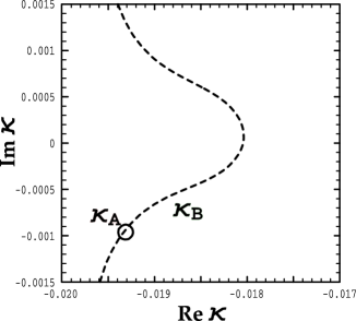
FIG. 1.: The relations between Eqs.(2.13) and (2.14) on the complex plane of $\kappa$. The solid (dotted) line shows the solution of Eq.(2.13) (Eq.(2.14)).

REFERENCES

- [1] K.S. Babu and R.N. Mohapatra, Phys. Rev. Lett. 70 2845 (1993); D-G Lee and R.N. Mohapatra, Phys. Rev. D51 1353 (1995).
- [2] K. Oda,E. Takasugi,M. Tanaka and M. Yoshimura, Phys. Rev. D59 055001 (1999).
- [3] H. Georgi and C. Jarlskog, Phys. Rev. B86 297 (1979).
- [4] T. P. Cheng, E. Eichten, and L. F. Li, Phys. Rev. D9, 2259 (1974); M. Marchacek and M. Vaughn, Nucl. Phys. B236, 221 (1984); M. Olechowski and S. Pokorski, Phys. Lett. B257, 388 (1991); H. Arason et al., Phys. Rev. D46, 3945 (1992); V. Barger, M. S. Berger, and P. Ohmann, Phys. Rev. D47, 1093 (1992).
- [5] H. Fusaoka and Y. Koide, Phys. Rev. D57, 3986 (1998).
- [6] D. E. Groom et al., The European Physical Journal C15, 1 (2000).
- [7] S. Weinberg, Ann. N. Y, Acad. Sci. 38, 185 (1977); H. Fritzsch, Phys. Lett. 73B, 317 (1978); Nucl. Phys. B155, 189 (1979); H. Georgi and D. V. Nanopoulos, ibid. B155, 52 (1979).
- [8] B. Brahmachari and R.N. Mohapatra, Phys. Rev. D58 015001 (1998).