Dissertation

submitted to the

Combined Faculties for the Natural Sciences and for Mathematics

of the Rupertus Carola University of

Heidelberg, Germany

for the degree of

Doctor of Natural Sciences

QCD coherence effects in high energy reactions with nuclei
presented by

Diplom-Physicist	Jörg Raufeisen
born in	Minden, Germany

Heidelberg, 12. Juli 2000
Referees: Prof. Dr. Jörg Hüfner Prof. Dr. Andreas Schäfer

Zusammenfassung

In dieser Arbeit werden Kohärenzeffekte in der tiefinelastischen Streuung (DIS) und im Drell-Yan (DY) Prozess an Kernen untersucht, insbesondere der Shadowing Effekt. Es wird im Ruhesystem des Targets und in der Farbdipol Formulierung gearbeitet. Die Glauber-Gribov Theorie für Mehrfachstreuung im Kern wird so modifiziert, dass der Formfaktor des Kernes in allen Streutermen berücksichtigt ist. Ferner wird die mittlere Kohärenzlänge für einen Fockzustand definiert. Damit ist es möglich abzuschätzen, dass das Gluon-Shadowing für $x_{Bj}>0.01$ vernachlässigbar ist. Parameter freie Rechnungen werden mit Daten von NMC und E665 für DIS und mit E772 Daten für DY verglichen. In beiden Fällen wird gute Übereinstimmung festgestellt. Der von HERMES beobachtete Effekt kann jedoch nicht reproduziert werden. Für DY-Dileptonen aus Proton-Kern Kollisionen bei RHIC Energien wird für den gesamten $x_{F}$ Bereich deutliches Shadowing vorrausgesagt. Der Einfluss des Kerns auf die Transversalimpuls-Verteilung der DY Paare wird ebenfalls untersucht. Des weiteren wird eine neue Parametrisierung des Dipol-Wirkungsquerschnittes präsentiert.

Abstract

In this work, coherence effects in deep inelastic scattering (DIS) and in the Drell-Yan (DY) process off nuclei are investigated, in particular nuclear shadowing. The target rest frame and the color dipole formulation are employed. Multiple scatterings are treated in Glauber-Gribov theory, which is modified to include the nuclear form factor to all orders. Based on the mean coherence length, which is defined in this work, it is estimated that gluon shadowing is negligible at $x_{Bj}>0.01$. Parameter free calculations are compared to NMC and E665 data for DIS and to E772 data for DY. In both cases, good agreement is found. It is however not possible to reproduce the effect observed by HERMES. For dileptons in proton-nucleus collisions at RHIC energies, considerable shadowing for the whole $x_{F}$ range is predicted. The influence of the nucleus on the DY transverse momentum distribution is also studied. Furthermore, a new parametrization of the dipole cross section is presented.

…all exact science is dominated by the idea of approximation.
Bertrand Russel

1 Introduction

The use of nuclei instead of protons in high energy scattering experiments, like deep inelastic scattering, provides unique possibilities to study the space-time development of strongly interacting systems. In experiments with proton targets the products of the scattering process can only be observed in a detector which is separated from the reaction point by a macroscopic distance. In contrast to this, the nuclear medium can serve as a detector located directly at the place where the microscopic interaction happens. As a consequence, with nuclei one can study coherence effects in QCD which are not accessible in DIS off protons nor in proton-proton scattering. An important question that can only be answered with the help of nuclei is for instance, how quarks and gluons evolve from the early stages of a collision to the hadrons which are finally observed in the detector. The large extension of the nuclear medium makes it possible to investigate, by which time scales this hadronization process is governed. Note that the radius of a heavy nucleus like lead is approximately eight times as large ($\approx 6.8$ fm in the nuclear rest frame) as the radius of a proton ($\approx 0.86$ fm).

This work is mostly concerned with the theoretical analysis of coherence effects in DIS off nuclei and in Drell-Yan (DY) dilepton production in proton-nucleus scattering, in particular with the phenomenon of nuclear shadowing. Before we turn to nuclear targets, we shortly review the physics of a proton target.

In DIS, a lepton is scattered off the target. This lepton radiates a virtual photon, which can resolve the microscopic substructure of the proton. Therefore, the huge colliders like HERA, where such experiments are performed, are big microscopes that allow to investigate, how the proton is made up of quarks. It is well known today that the proton contains three quarks which are called valence quarks. These valence quarks carry the quantum numbers of the proton and are the analog of the valence electrons which are responsible for the chemical properties of an atom. In addition to the quarks, there are also gluons inside the proton. Gluons mediate the color forces between the quarks. Since gluons have no electromagnetic charge they are not directly observable in DIS. One can however conclude that there must be neutral partons in the proton since quarks carry only about half of the momentum of the proton. The missing momentum is believed to be carried by gluons. It is natural to ask, whether quarks and gluons are elementary or whether they have a substructure themselves. In order to find an answer to this question, one has to increase the resolution of the microscope, i.e. build colliders with higher energies which can measure at higher momentum transfer. Today, the highest energies are reached at HERA where positrons collide with protons at a center of mass (c.m.) energy $\sqrt{S}\approx 300$ GeV. As the resolution is increased, one finds that a quark, carrying the longitudinal momentum fraction Bjorken-$x_{Bj}$ of the proton consists of a quark and a gluon which carry both together the momentum of the parent quark and therefore each a smaller momentum fraction of the proton. In addition, also gluons can split into quark-antiquark ($q\bar{q}$) pairs. This is confirmed experimentally by the increase of the quark density at low values of $x_{Bj}<0.1$. At very low $x_{Bj}\ll 0.1$, the partonic content of the proton is dominated by gluons and the photon sees only the $q\bar{q}$-pairs which originate from gluon splitting. However, one cannot distinguish in DIS whether the virtual photon couples to a quark or to an antiquark. Complementary information about the antiquark density is provided by the Drell-Yan (DY) process. In the DY process in proton-proton collisions, a quark from the projectile can annihilate with an antiquark from the target and produce a massive photon. This photon decays into a lepton pair which can be detected.

How does a nucleus look like at high energies, i.e. at low $x_{Bj}$? The answer depends on the reference frame. In a frame where the nucleus is fast moving, the so-called infinite momentum frame, the nucleus is strongly Lorentz contracted. However, the localization of gluons which carry only a very small momentum fraction of the nucleus is determined by the uncertainty principle. In the infinite momentum frame, the cloud of these low-$x_{Bj}$ gluons extends over the whole nucleus and the nucleons are able to communicate with each other. The situation looks different in the rest frame of the nucleus. In the nuclear rest frame, the nucleons are well separated from each other by a distance of $\sim 2$ fm. How can these two pictures, infinite momentum frame and rest frame, be reconciled with each other? Of course, all observables have to be Lorentz invariant.

Figure 1: At low $x_{Bj}$ and in the target rest frame, the virtual photon converts into a $q\bar{q}$-pair long before the target. The quark carries momentum fraction $\alpha$ of the $\gamma^{*}$, the antiquark $1-\alpha$. The transverse separation between the particles is denoted by $\rho$. The curly line represents a gluon.

Note that not only the partonic structure of the nucleus is frame depended, but also the partonic interpretation of the scattering process. At high energies, nuclear scattering is governed by coherence effects which are most easily understood in the target rest frame. In the rest frame, DIS looks like pair creation from a virtual photon, see fig. 1. Long before the target, the virtual photon splits up into a $q\bar{q}$-pair. The lifetime $l_{c}$ of the fluctuation can be estimated with help of the uncertainty relation to be of order $\sim 1/m_{N}x_{Bj}$ (cf. section 2.3) where $m_{N}\approx 1$ GeV is the mass of a nucleon. The coherence length can become much greater than the nuclear radius at low $x_{Bj}$. On a nuclear target, the pair will experience multiple scatterings off different nucleons within the coherence length. This corresponds to the overlap of gluon clouds from different nucleons in the infinite momentum frame. The long lifetime of the $q\bar{q}$ fluctuation, which extends over the whole nucleus, leads to the pronounced coherence effects observed in experiment. The measurable cross section is independent of the reference frame, but our physical picture depends on it. The target rest frame is especially well suited for the study of coherence effects.

The most prominent example for a coherent interaction of more than one nucleon is the phenomenon of nuclear shadowing. Naively one would expect that the cross section for scattering a lepton off a nucleus with mass number $A$ is $A$ times as large as the cross section for scattering the lepton off a proton. In experiment it is however seen that the nuclear cross section is significantly smaller. Shadowing in low $x_{Bj}$ DIS and at high photon virtualities was first observed by the EM collaboration [2]. The same reduction of the cross section was measured by E772 for the Drell-Yan (DY) process at low $x_{2}$ [3].

What is the mechanism behind this suppression? If the coherence length is very long, as indicated in fig. 1, the $q\bar{q}$-dipole undergoes multiple scatterings inside the nucleus. The physics of shadowing in DIS is most easily understood in a representation, in which the pair has a definite transverse size $\rho$. As a result of color transparency [4, 5, 6], small size pairs interact with a small cross section $\sigma_{q\bar{q}}(\rho)$, while large pairs interact with a large cross section. The term ”shadowing” can be taken literally in the target rest frame. The large pairs are absorbed by the nucleons at the surface which cast a shadow on the inner nucleons. The small pairs are not shadowed. They can propagate through the whole nucleus. From these simple arguments, one can already understand the two most important conditions for shadowing. First, the hadronic fluctuation of the virtual photon has to interact with a large cross section and second, the coherence length has to be long enough to allow for multiple scattering. At $x_{Bj}\to 0$ the coherence length becomes infinite and shadowing in DIS can be calculated from a formula very similar to the Glauber-Gribov eikonal formula [7, 8], if one knows the cross section $\sigma_{q\bar{q}}(\rho)$ for scattering a $q\bar{q}$-pair with transverse size $\rho$ off a nucleon. The application of the eikonal formula is possible because at infinitely high energies $q\bar{q}$-dipoles with fixed separation in impact parameter space are eigenstates of the interaction [4, 9, 10]. The dipole cross section is the main nonperturbative ingredient to all calculations in this work.

Nuclear shadowing has received much attention within the last two decades. A detailed review of different approaches to nuclear shadowing can be found in [11], see also the more recent review [12].

Note however that shadowing has not yet been measured at RHIC ($\sqrt{S}\approx 200$ GeV) nor LHC ($\sqrt{S}\approx 5.5$ TeV) energies. Furthermore, it is only known for quarks. Shadowing is also expected for the nuclear gluon distribution. This gluon shadowing could have a strong influence on the expected quark gluon plasma formation at RHIC and LHC and is only poorly understood at present. Only quark shadowing is calculated in this work, but the light-cone approach can also be extended to gluon shadowing [13]. Further insight into the physics of nuclear parton distributions could be provided by DIS experiments off nuclei at eRHIC or at HERA. Nuclei could also be included into the THERA option at TESLA ($\sqrt{S}\approx 1.4$ TeV). The advantage of using nuclear targets is that parton densities which could be probed only at LHC energies with proton targets are already accessible at HERA energies. Such experiments are not only important in view of the quark gluon plasma. They can also clarify, up to which energies the QCD improved parton model can be applied.

Figure 2: In the target rest frame, DY dilepton production looks like bremsstrahlung. A quark or an antiquark inside the projectile hadron scatters off the target color field and radiates a massive photon, which subsequently decays into the lepton pair. The photon can also be radiated before the quark hits the target.

While the target rest frame picture of DIS is very popular, the light-cone approach of Kopeliovich [14, 15, 16], which describes the DY process in the target rest frame, is less known. In the light-cone approach, DY dilepton production in the rest frame of the target appears as bremsstrahlung, see fig. 2. A quark from the projectile scatters off the target and radiates a virtual photon. This photon decays into a lepton pair. Remarkably, the DY cross section can be expressed in terms of the same dipole cross section that appears in DIS, cf. section 2.6. This is a result of the QCD factorization theorem [15]. On a nuclear target, the quark will of course scatter several times. The effect of multiple scattering on bremsstrahlung is well known in QED as the Landau-Pomeranchuk-Migdal (LPM) effect [17, 18, 19], see also [20]. The LPM effect leads to a reduction of the cross section due to destructive interferences in multiple scattering within an amorphous medium. An electron incident on a dense target with $n$ scattering centers, will radiate bremsstrahlung after the first scattering. If the electron energy (in QED) is high enough, the longitudinal momentum transfer in a single interaction is small and according to the uncertainty relation, the electron needs a long time to recreate it’s electromagnetic field. Within this coherence time, the electron can travel macroscopic distances. This is in complete analogy to the case of DIS. If the electron is hit several times within this length, it cannot radiate again, because it has not yet recreated it’s field. Therefore, the overall cross section is less than $n$ times the single scattering cross section. It is remarkable that a microscopic process, where all momenta are large, can exhibit a length scale of order millimeters (in QED).

Note that both, shadowing in DIS and DY, can be calculated from the Glauber eikonal formula at infinitely high energies, where the transverse motion of the particles in the pair, fig. 1, or the incident quark, fig. 2, can be neglected. In this work, a Green function approach is developed that allows to do calculations at energies which can be reached in experiment.

Note that shadowing in DIS can also be regarded as LPM effect for pair production. The physical interpretation is however much less intuitive. Both processes, bremsstrahlung and pair production, were studied in [19]. After the experimental discovery of the LPM effect for bremsstrahlung in QED [21, 22, 23], more than forty years after its theoretical prediction, this effect again received much attention. In particular the QCD variant of the LPM effect was extensively studied with respect to suppression of gluon radiation and energy loss of particles propagating in a quark gluon plasma. The two most important approaches are the path integral approach by Zakharov [24]-[30] and the diagrammatic technique of the BDMPS collaboration [31]-[37]. It is demonstrated in [37] that the two formulations are equivalent. Further work on the LPM effect in heavy ion collisions is done in [38, 39, 40]. A review of the present theoretical understanding of the LPM effect can be found in [41]. The formulation of nuclear shadowing presented in this work is the one of Zakharov since our both approaches are extensions of Glauber-Gribov theory. The treatment of shadowing in DIS as LPM effect was first suggested in [28] and elaborated in [42, 43].

This work mainly consists of two parts. In the first part, section 2, DIS and diffraction on a proton target and DY dilepton production in proton-proton scattering are considered. The deep inelastic structure functions and the definitions of kinematical variables are introduced in section 2.1. In section 2.2, the parton model and the QCD improved parton model are shortly reviewed. The first two sections can be skipped by a reader familiar with these concepts. The space-time picture of low $x_{Bj}$ DIS in the color dipole formulation is discussed in some detail in section 2.3. The basic concepts of the light-cone approach and the techniques for treating nonperturbative effects, which are employed throughout this work, are presented in this section, too. Section 2.4 is a continuation of the preceding section and contains a discussion of diffraction in the color dipole picture. The sections 2.5 and 2.6 treat the DY process. While in section 2.5 the well known parton model of the DY process is shortly explained, section 2.6 introduces the color dipole formulation of the DY process. This formulation is employed in section 3 where nuclear targets are considered. Finally, a new parametrization of the dipole cross section is presented in section 2.7. All results of numerical calculations for proton targets and comparison with experimental data are shown in this section.

The light-cone approach is extended to nuclear targets in section 3. This section contains the main results of this work. The connection between nuclear shadowing in DIS and diffraction is discussed in section 3.1. In addition, the Glauber-Gribov multiple scattering theory is shortly introduced and the physical conditions which have to be fulfilled in order to observe shadowing are explained. In the sections 3.2 and 3.3, it is explained how the nuclear form factor can be introduced in all multiple scattering terms. While section 3.2 is intended to explain the physics of our approach, a more formal derivation and a discussion of approximations which are employed is given in section 3.3. The mean coherence length is defined in section 3.4. This quantity is intended to be a tool for qualitative considerations. In section 3.5 an estimate is given, on how many dilepton pairs in the low mass region are produced via the bremsstrahlungs-mechanism. Proton-nucleus and nucleus-nucleus collisions are considered in this section, but no shadowing is taken into account. Shadowing for DY dilepton production is discussed in section 3.6, where also predictions for RHIC are presented. Section 3.7 contains the comparison of our calculation with data for shadowing in DIS and DY.

2 Soft contributions to hard QCD reactions

Deep inelastic scattering (DIS) and the Drell-Yan (DY) process are the two classical examples for the application of perturbative QCD (pQCD). The high virtuality of the photon or the large mass of the dilepton pair, respectively, provides the hard scale, which is necessary for perturbation theory. Due to confinement, the fundamental QCD degrees of freedom, quarks and gluons are not directly observable but occur only in bound states. Therefore all QCD reactions also involve a soft scale, given e. g. by the radius of the hadron.

Such two-scale processes have been extensively studied for more than 20 years and their theoretical treatment has reached a high level of sophistication. Basic to the standard approach is the operator product expansion (OPE), invented by Wilson [44]. Combined with asymptotic freedom, the OPE is a systematic way to separate hard and soft scales in DIS, DY and other hard processes. The observable cross sections can be written in factorized form, namely as a convolution of a hard partonic cross section and of the soft parton distribution of the hadrons (or of hadronic matrix elements, more generally speaking). Contributions which do not factorize vanish in the limit $Q^{2}\to\infty$. While the partonic cross section is governed by the hard scale and can be calculated perturbatively, the parton distributions are of completely nonperturbative origin and no way is known to calculate them from QCD. Even lattice calculations are not applicable in the kinematical region of DIS and DY.

Instead, the parton distributions have to be extracted from experimental data. Their most important property is, that they are independent of the particular hard process under consideration and depend only on the hadron. This universality is crucial to make the theory predictive. Today, several collaborations exist which provide parametrizations of these distributions [45, 46, 47]. The parton distributions are typically given at a semihard input scale $Q_{0}^{2}$. The evolution of the parton distributions to higher virtuality $Q^{2}$ is then correctly described by the DGLAP evolution equations [48]-[51]. This is one of the great successes of QCD and an important argument, that QCD is the correct field theory of the strong interaction.

One should however bear in mind, that the soft physics is completely described in terms of fit functions and nothing is known about the nonperturbative mechanisms, leading to the specific shape of the parton distributions. In particular, all coherence effects, which are so important in high energy nuclear physics, are hidden in these parametrizations. The aim of this work is to develop an approach which makes the physics underlying these coherence effects transparent and intuitively understandable.

The purpose of this sections is to introduce the basics of the light-cone approach to DIS and DY before nuclear targets are considered in section 3. The fundamental input to all calculations is the cross section for scattering a quark-antiquark dipole off a proton. A parametrization of the dipole cross section is presented, which describes well all $F_{2}$ data from H1 and ZEUS at $Q^{2}\leq 35$ GeV² and also reproduces total hadronic cross sections. We do not aim to achieve the same level of sophistication as the OPE approach in this work. We rather intend to develop a good physical understanding of high energy DIS and DY in the framework of the light-cone approach, which is especially well suited to describe coherence effects in multiple scattering off nuclei. This section also serves as a reminder of the definition of structure functions and kinematical variables.

2.1 Description of DIS in terms of structure functions

The natural language to describe hard QCD processes is based on structure functions which contain all information about the substructure of the target. These functions are defined by relating them to the experimentally observable lepton-target cross section and can be expressed in terms of hadronic matrix elements. They acquire a physical interpretation within a parton model of the structure of the target. The definition of structure functions in DIS is explained in more detail in standard textbooks, see e. g. [52, 53, 54], we will only give a short overlook. Only the scattering of charged leptons is discussed in this work. Deep inelastic neutrino scattering, as well as $Z_{0}$ exchange are not considered.

Figure 3: Inclusive deep-inelastic lepton-proton scattering. A charged lepton with four-momentum $k^{\mu}=(E,\vec{k})$ scatters off a proton with four-momentum $P^{\mu}=(E_{p},\vec{P})$. In DIS a spacelike photon with momentum $q^{2}=-Q^{2}<0$ is exchanged. Only the scattered lepton with momentum $k^{\mu\prime}$ is observed in inclusive measurements.

The kinematics for inclusive DIS is explained in fig. 3. A lepton scatters off a proton or a nucleus. Due to the impact of the virtual photon, the target breaks up into an unobserved final state $X$. Only the scattered lepton is observed in the final state. We work with the standard kinematical variables. The virtuality of the photon is denoted by

$$Q^{2}=-q^{2}=(k-k^{\prime})^{2}>0$$ (1)

and the mass of a proton by

$$m_{N}^{2}=P^{2}\approx 1~{}{\rm GeV}^{2}.$$ (2)

Furthermore the lepton-nucleon center of mass (cm) energy squared is defined as

$$S=(k+P)^{2}$$ (3)

and the same for the $\gamma^{*}$-nucleon system

$$s=(q+P)^{2}.$$ (4)

For convenience, we have chosen our convention slightly different from the standard convention, where $s$ is denoted by $W^{2}$. The Bjorken variable is given by

$$x_{Bj}=\frac{Q^{2}}{2P\cdot q}=\frac{Q^{2}}{2m_{N}\nu}\approx\frac{Q^{2}}{Q^{2}+s}$$ (5)

and the relative energy loss of the lepton is

$$y=\frac{P\cdot q}{P\cdot k}\approx\frac{Q^{2}+s}{S}.$$ (6)

We will also frequently use the Lorentz invariant variable

$$\nu=\frac{P\cdot q}{m_{N}}.$$ (7)

In one photon exchange approximation, the differential cross section for inclusive scattering reads

$$d\sigma(eP\to e^{\prime}X)=\frac{1}{2S}\frac{d^{3}k^{\prime}}{(2\pi)^{3}2E^{\prime}}\sum_{X}(2\pi)^{4}\delta^{4}(P+k-p_{X}-k^{\prime})|{\cal{A}}|^{2}.$$ (8)

The sum over final states is understood to include also the integration over phase space. The absolute square of the matrix element reads

$$|{\cal{A}}|^{2}=\frac{4\pi\alpha_{em}}{Q^{4}}l_{\mu\nu}\langle P|J^{\mu\dagger}(0)|X\rangle\langle X|J^{\nu}(0)|P\rangle$$ (9)

after summation of the polarizations of the virtual photon and in one photon exchange approximation. Here, $J^{\mu}$ is the electromagnetic current. The leptonic tensor is known as

$$l_{\mu\nu}=2(k^{\prime}_{\mu}k_{\nu}+k^{\prime}_{\nu}k_{\mu}-g_{\mu\nu}k^{\prime}\cdot k).$$ (10)

We have averaged over spins of the initial lepton and summed over the final spins. All information about the target resides now in the hadronic tensor defined by

$$W^{\mu\nu} = \sum_{X}\langle P|J^{\mu}(0)|X\rangle\langle X|J^{\nu}(0)|P\rangle(2\pi)^{4}\delta^{4}(P+q-p_{X})$$ (11)

$$= \int d^{4}x{\rm e}^{{\rm i}qx}\langle P|J^{\mu}(x)J^{\nu}(0)|P\rangle.$$ (12)

In order to obtain (12), one has to make use of the integral representation of the $\delta$-function and of the completeness of the final hadronic states $X$. The hadronic tensor is then related to the discontinuity of the forward virtual Compton scattering amplitude $T^{\mu\nu}$ via

$$W^{\mu\nu}=\frac{1}{2\pi}{\rm Disc}T^{\mu\nu}=\lim_{\varepsilon\to 0}\frac{1}{4\pi{\rm i}}(T^{\mu\nu}(q_{0}+{\rm i}\varepsilon)-T^{\mu\nu}(q_{0}-{\rm i}\varepsilon)),$$ (13)

with

$$T^{\mu\nu}={\rm i}\int d^{4}x{\rm e}^{{\rm i}qx}\langle P|{\cal T}(J^{\mu}(x)J^{\nu}(0))|P\rangle.$$ (14)

Here, ${\cal T}$ is the time ordering operator. Note that the discontinuity of $T$ equals the imaginary part of $T$ since the current operators $J^{\mu}$ are hermitian. As illustrated in fig. 4, the relation between the hadronic tensor and the Compton amplitude is a manifestation of the optical theorem.

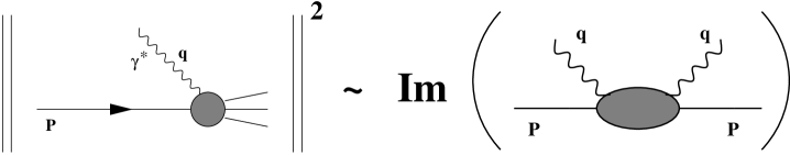
Figure 4: The hadronic tensor $W^{\mu\nu}$ is related to the imaginary part of the forward ($P=P^{\prime}\;,\;q=q^{\prime}$), virtual ($Q^{2}>0$) Compton scattering amplitude via the optical theorem.

Making use of Lorentz covariance, gauge invariance and parity conservation, one finds that the most general structure of $W^{\mu\nu}$ is

$$W^{\mu\nu}=\left(-g^{\mu\nu}+\frac{q^{\mu}q^{\nu}}{q^{2}}\right)W_{1}(x_{Bj},Q^{2})+\left(P^{\mu}+\frac{q^{\mu}}{2x_{Bj}}\right)\left(P^{\nu}+\frac{q^{\nu}}{2x_{Bj}}\right)W_{2}(x_{Bj},Q^{2}).$$ (15)

The dimensionless invariant structure functions for DIS are commonly defined as

$$F_{1}(x_{Bj},Q^{2}) = W_{1}(x_{Bj},Q^{2}),$$ (16)

$$F_{2}(x_{Bj},Q^{2}) = \nu W_{2}(x_{Bj},Q^{2})$$ (17)

and with this notation, the cross section for $ep\to e^{\prime}X$ reads

$$\frac{d^{2}\sigma}{dx_{Bj}dQ^{2}}=\frac{4\pi\alpha_{em}^{2}}{Q^{4}}\left\{\left(1-y-\frac{x_{Bj}^{2}y^{2}m_{N}^{2}}{Q^{2}}\right)\frac{F_{2}(x_{Bj},Q^{2})}{x_{Bj}}+y^{2}F_{1}(x_{Bj},Q^{2})\right\}.$$ (18)

Since the only purpose of the lepton is to radiate the virtual photon, it is convenient to think about DIS as $\gamma^{*}p$-scattering and to define corresponding cross sections for transverse and longitudinal photons. The cross section for a virtual photon with helicity $\lambda$ can be defined as

$$\sigma_{\lambda}=\frac{4\pi^{2}\alpha_{em}}{K}\epsilon_{\mu}(\lambda)\epsilon_{\nu}^{*}(\lambda)\,{\rm Im}T^{\mu\nu}.$$ (19)

Note that the flux factor of a virtual photon is not well defined. We employ the convention of Hand [55], i. e.

$$K=2P\cdot q-Q^{2}\approx 2s.$$ (20)

With this convention one obtains

$$\sigma_{T} = \frac{4\pi^{2}\alpha_{em}}{Q^{2}(1-x_{Bj})}2x_{Bj}F_{1}(x,Q^{2}),$$ (21)

$$\sigma_{L} = \frac{4\pi^{2}\alpha_{em}}{Q^{2}(1-x_{Bj})}\left[\left(1+\frac{Q^{2}}{\nu^{2}}\right)F_{2}(x_{Bj},Q^{2})-2x_{Bj}F_{1}(x_{Bj},Q^{2})\right].$$ (22)

Here, $\sigma_{T}$ is the cross section for transverse photons and $\sigma_{L}$ for longitudinal photons. One also often introduces the helicity structure functions,

$$F_{T}(x_{Bj},Q^{2}) = \frac{Q^{2}(1-x_{Bj})}{4\pi^{2}\alpha_{em}}\sigma_{T},$$ (23)

$$F_{L}(x_{Bj},Q^{2}) = \frac{Q^{2}(1-x_{Bj})}{4\pi^{2}\alpha_{em}}\sigma_{L}.$$ (24)

The invariant structure functions $F_{1}$ and $F_{2}$ can be expressed in terms of the helicity structure functions $F_{T}$ and $F_{L}$ and vice versa. In particular, one obtains in the Bjorken limit, $Q^{2}\to\infty$, $x_{Bj}$ fixed,

$$F_{2}(x_{Bj},Q^{2}) = F_{T}(x_{Bj},Q^{2})+F_{L}(x_{Bj},Q^{2})$$ (25)

$$F_{1}(x_{Bj},Q^{2}) = \frac{F_{T}(x_{Bj},Q^{2})}{2x_{Bj}}.$$ (26)

There are only two independent structure functions in DIS off unpolarized targets.

2.2 The parton model of DIS

It came as a big surprise, when the first DIS measurements at SLAC [56] showed that the structure function $F_{2}(x_{Bj},Q^{2})$ is nearly constant as function of $Q^{2}$ at fixed $x_{Bj}$. An explanation of this phenomenon was given by Bjorken [57] and by Feynman [58]. Feynman’s intuitive explanation is depicted in fig. 5a. He proposed that the proton is made up of pointlike charged constituents, so called partons, and the total $\gamma^{*}p$ cross section is the incoherent sum of photon-parton cross sections. The transverse momenta of the partons are neglected, which is well justified in a frame where the proton is fast moving, e. g. in the Breit frame or in the infinite momentum frame [59]. In such a frame the longitudinal momenta of the partons are much larger than the transverse ones.

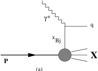
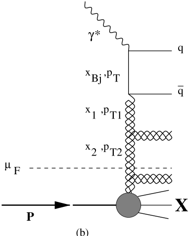
Figure 5: The parton model for DIS (a) and its QCD improvement (b). In the naive parton model, the virtual photon hits a quark (q) inside the target. In the QCD improved parton model, the quark can e. g. be created from a gluon, denoted by a curly line, by the splitting process $G\to q\bar{q}$. The $x_{i}$ are the longitudinal momentum fractions of the particles with respect to the target. Therefore $x_{Bj}<x_{1}<x_{2}<\dots$.

The cross sections for transverse and longitudinal photons scattering off spin-$1/2$ partons, i. e. quarks (fig. 5a), are given by

$$\sigma_{T}^{\gamma^{*}q} = \frac{4\pi^{2}\alpha_{em}Z_{f}^{2}}{Q^{2}(1-x_{Bj})}\delta\left(1-\frac{x_{Bj}}{x_{q}}\right)$$ (27)

$$\sigma_{L}^{\gamma^{*}q} = 0,$$ (28)

where $x_{q}$ is the momentum fraction of the proton carried by the struck quark and $Z_{f}$ is the flavor charge in units of the elementary charge. The $\delta$-function arises from momentum conservation and gives a physical meaning to the Bjorken variable. In the Breit frame, $x_{Bj}$ is the momentum fraction of the proton carried by the struck quark. For massless quarks, the longitudinal cross section is zero due to helicity conservation. Introducing the density $q_{f}(x_{Bj})$ of quarks of flavor $f$, inside the proton, one obtains a simple partonic interpretation of the structure functions,

$$F_{2}(x_{Bj}) = x_{Bj}\sum\limits_{f}Z_{f}^{2}(q_{f}(x_{Bj})+\bar{q}_{f}(x_{Bj})),$$ (29)

$$F_{L} = 0.$$ (30)

In the naive parton model, the structure functions depend only on $x_{Bj}$ and not on $Q^{2}$, the longitudinal structure function vanishes and one obtains the Callan-Gross relation [60],

$$F_{2}-2x_{Bj}F_{1}=0.$$ (31)

These equations are the basic results of the parton model and they are approximately confirmed by experiment.

One of the great achievements of QCD is the successful description of the deviations from the naive parton model seen in experiment. In particular at low $x_{Bj}$ deviations from Bjorken scaling become quite pronounced, see fig. 6. In the QCD improved parton model, perturbation theory is applied to calculate corrections to the parton model predictions. An example of such a correction, which is important at low $x_{Bj}$, is shown in fig. 5b. The quark seen by the photon is generated perturbatively from a gluon by the splitting process $G\to q\bar{q}$. Higher order corrections allow also to take into account further gluons radiated from the gluon that splits into the $q\bar{q}$-pair.

Figure 6: Deviations from Bjorken scaling can be explained by pQCD corrections to the naive parton model. While Bjorken scaling is approximately fulfilled at high $x_{Bj}$, scaling violations become stronger and stronger as $x_{Bj}$ decreases. At very low $x_{Bj}$, practically no scaling can be observed any more. The figure is taken from [12] and the data are from ZEUS [61, 62], E665 [63] and NMC [64].

The evolution of the structure function with $Q^{2}$ is described by the DGLAP equations. There are several ways to motivate these equations. The DGLAP evolution equations resum logarithms in $Q^{2}$ originating from ladder diagrams like the one in fig. 5b. Historically, they originate from a time even before QCD. Gribov and Lipatov [48, 49] were the first who found that these ladder diagrams receive dominant contributions from configurations with strong ordering in the transverse momenta, i.e.

$$p_{T1}^{2}\gg p_{T2}^{2}\gg\dots.$$ (32)

They obtained integrals of the form $dp_{T}^{2}/p_{T}^{2}$ which could be resummed to all orders. However, their calculations were done in an abelian theory. A very intuitive derivation in non-covariant Hamiltonian perturbation theory was given later (in QCD) by Altarelli and Parisi [50]. The illustrative interpretation of the DGLAP equations is due to them. The photon acts as a microscope with a resolution determined by $Q^{2}$. As one increases $Q^{2}$, the photon resolves more and more of the target substructure. The probability to find a quark and an antiquark of flavor $f$ inside a gluon, fig. 5b, is then described by a splitting function $P_{fG}$. Similarly, there exists a splitting function which describes the probability to find a quark and another gluon inside the parent gluon. Finally, Dokshitzer [51] derived the same equation again with the method proposed by Gribov and Lipatov, but now in QCD.

From the process where the quark seen by the photon is generated by the splitting of a gluon, one obtains in perturbation theory the contribution

$$\frac{F_{2}(x_{Bj},Q^{2})}{x_{Bj}} = \sum\limits_{f}Z_{f}^{2}\Bigg{[}q_{f}\left(x_{Bj}\right)$$ (33)

$$+ \frac{\alpha_{s}}{2\pi}\int\limits_{x_{Bj}}^{1}\frac{dx_{1}}{x_{1}}G(x_{1})\left\{P_{fG}\left(\frac{x_{Bj}}{x_{1}}\right)\ln\left(\frac{Q^{2}}{\kappa^{2}}\right)+\dots\right\}\Bigg{]}$$

to the structure function. Here, $G(x_{1})$ ist the gluon density of the target and $x_{Bj}/x_{1}\leq 1$ is the momentum fraction of the gluon carried away by the quark in the ladder. The logarithmic divergence in (33) is regularized by the cutoff $\kappa$. The dots denote renormalization scheme dependent functions which can be calculated and contain no such divergence. These functions are of no interest to our more qualitative discussion and we refer to [53] for more details. The splitting function is given by

$$P_{fG}(z)=\frac{1}{2}\left[z^{2}+(1-z)^{2}\right].$$ (34)

The divergence in (33) is a collinear divergence, originating from configurations with $p_{T}\to 0$ in fig. 5b. This limit corresponds to a long range part of the strong interaction which cannot be calculated in perturbation theory. Therefore, the quark ($q_{f}$) and gluon ($G$) densities in (33) are unmeasurable, bare parton distributions, $q_{f0}$ and $G_{0}$. The renormalized quark density may be defined as

$$q_{f}(x_{Bj},\mu_{F})=q_{f0}(x_{Bj})+\frac{\alpha_{s}}{2\pi}\int_{x_{Bj}}^{1}\frac{dx_{1}}{x_{1}}G_{0}(x_{1})\left\{P_{fG}\left(\frac{x_{Bj}}{x_{1}}\right)\ln\left(\frac{\mu_{F}^{2}}{\kappa^{2}}\right)+\dots\right\}.$$ (35)

The collinear singularity is absorbed into the bare quark density at the factorization scale $\mu_{F}$. With this prescription, the partonic interpretation of $F_{2}$ (29) is maintained, but the structure function is no longer independent of $Q^{2}$.

The distribution $q_{f}(x_{Bj},\mu_{F})$ cannot be calculated in pQCD, since it is dominated by soft physics. It has to be extracted from measurements of $F_{2}$. However one can calculate in pQCD, how the parton distribution runs with the factorization scale. Since $\mu_{F}$ is not a physical quantity, observables cannot depend on it. Therefore,

$$\frac{dF_{2}(x_{Bj},Q^{2},\mu_{F})}{d\mu_{F}}=0$$ (36)

and

$$Q^{2}\frac{dq_{f}(x_{Bj},Q^{2})}{dQ^{2}}=\frac{\alpha_{s}}{2\pi}\int_{x_{Bj}}^{1}\frac{dx_{1}}{x_{1}}P_{fG}\left(\frac{x_{Bj}}{x_{1}}\right)G(x_{1},Q^{2}).$$ (37)

This is one of the DGLAP equations which describes the evolution of the quark density.

Note that also the gluon density depends on $Q^{2}$, because of pQCD corrections. Altogether one obtains $N_{f}+1$ coupled equations describing the $Q^{2}$ evolution of the singlet parton densities,

$$Q^{2}\frac{d}{dQ^{2}}\left(\begin{array}[]{c}q_{f}(x_{Bj},Q^{2})\\[10.00002pt] G(x_{Bj},Q^{2})\end{array}\right)=\frac{\alpha_{s}}{2\pi}\int\limits_{x_{Bj}}^{1}\frac{dx_{1}}{x_{1}}\left(\begin{array}[]{cc}P_{ff}\left(\frac{x_{Bj}}{x_{1}}\right)&P_{fG}\left(\frac{x_{Bj}}{x_{1}}\right)\\[10.00002pt] P_{Gf}\left(\frac{x_{Bj}}{x_{1}}\right)&P_{GG}\left(\frac{x_{Bj}}{x_{1}}\right)\end{array}\right)\left(\begin{array}[]{c}q_{f}(x_{1},Q^{2})\\[10.00002pt] G(x_{1},Q^{2})\end{array}\right),$$ (38)

How can one calculate $P_{Gf}$ and $P_{GG}$. The photon does not couple directly to gluons. The most straightforward way is to consider a longitudinal photon in fig. 5b. In this case, the $\alpha_{s}$ correction (33) does not contain a divergence and therefore does not contribute to the running of the quark densities. It is easy to understand intuitively, why there is no divergence for longitudinal photons. The divergence originates from configurations with $p_{T}\to 0$. This case however is exactly the naive parton model, in which $\sigma_{L}=0$ due to helicity conservation. In order to obtain $P_{Gf}$ and $P_{GG}$, one has to take into account at least one rung in the ladder. The splitting function is the coefficient of the logarithmic divergence occuring at $p_{T1}\to 0$. For this reason, longitudinal photons are often called ”gluonometer” [51].

At present the splitting functions are known to next to leading order in pQCD. They can e. g. be found in [52]. The function $P_{GG}(x_{Bj}/x_{1})\sim 6x_{1}/x_{Bj}$ (at low $x_{Bj}$) exhibits a pole at $x_{Bj}=0$. It is widely believed that this pole is responsible for the steep rise of $F_{2}$ and the high gluon density at low $x_{Bj}$, which behaves approximately like

$$x_{Bj}G(x_{Bj},Q^{2})\propto\exp\left(2\sqrt{\frac{N_{c}\alpha_{s}}{\pi}\ln(1/x_{Bj})\ln(Q^{2}/Q^{2}_{0})}\right)$$ (39)

for fixed strong coupling constant $x_{Bj}$. There are however also different opinions [65, 66].

DGLAP is a special kind of a renormalization group equation. One of its most important properties is that it separates scales. All the soft physics is contained in the parton distributions. These are of entirely nonperturbative origin and have to be parametrized at some input scale $Q_{0}^{2}$. Such parametrizations are provided by the three collaborations GRV, MRST and CTEQ [45, 46, 47] in leading and in next to leading order. With the parton distributions as input, one can then calculate $F_{2}$ at a higher value of $Q^{2}$, because the splitting functions can be calculated in pQCD. The other essential property is, that the parton distributions are universal, i. e. they do not depend on the process under consideration, but only on the hadron state.

A more rigorous technique to separate scales in QCD is Wilson’s operator product expansion [44]. Using the OPE, the matrix of anomalous dimensions, i.e. the Mellin transforms of the splitting functions, was derived by Georgi and Politzer [67] and by Gross and Wilcek [68]. Explaining the OPE is however not within the scope of this work and we rather refer to standard texts [54]. We only mention that in this method the time ordered product of currents in the virtual Compton amplitude (14) is expanded near the light cone in a series of local operators with coefficient functions which are singular on the light cone. These coefficient functions can be calculated in pQCD and are related to the splitting functions by Mellin transform. It is interesting to see within this framework, that (i) DIS is a long distance process receiving large contributions from the region near the lightcone, (ii) the partonic interpretation of $F_{2}$ is valid only in the infinite momentum frame and (iii) additional terms occur, which cannot be interpreted as parton densities. These are the so called higher twist terms which are formally expressed as matrix elements of multiple field correlators. A typical example is a double scattering process. These matrix elements are, like the parton densities, not accessible by means of perturbation theory and have to be adjusted to experimental data. The matrix elements are however universal, since they depend only on the state in which the field correlator is evaluated. Higher twists are typically suppressed by additional powers of $Q^{2}$, but can be enhanced by a factor $A^{1/3}$ in processes involving nuclei, where $A$ is the nuclear mass number. The $A$ enhancement was argued by Luo, Qiu and Sterman [69, 70]. The calculation of higher twist terms is rather involved and they are theoretically not well under control.

2.3 The color dipole picture of low-x DIS

In this section we have a closer look at the space time picture of DIS at low $x_{Bj}$. The two possible time orderings for the photon-quark interaction are depicted in fig. 7. In 7a, the virtual photon penetrates the target and hits a quark. In 7b however, the $\gamma^{*}$ splits up into a $q\bar{q}$ pair that subsequently scatters off the target color field. In covariant Feynman-perturbation theory, both contributions are automatically taken into account. It is however instructive to consider DIS in the target rest frame and in a Hamiltonian, i.e. not manifestly covariant, picture, because this will give us a clearer physical understanding of the dominant mechanism and in turn we can make full use of our physical intuition.

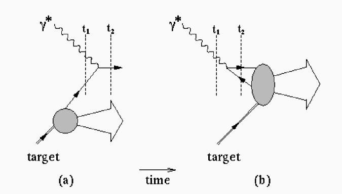
Figure 7: The two time orderings for the interaction of a virtual photon with a target: (a) The photon hits a quark inside the target, (b) the photon splits up into a $q\bar{q}$-pair which subsequently scatters off the target color field. In the rest frame of the target, the latter contribution is the dominant one. The figure is taken from [12].

The relative importance of the two contributions in fig. 7 may be estimated from the ratio of the energy denominators as it was done in [71]. For large photon energies, $\nu\gg m_{N}$, these energy denominators were found to be

$$\Delta E_{a} = E_{a}(t_{2})-E_{a}(t_{1})\approx-\langle p_{q}^{2}\rangle^{1/2}+\frac{\frac{2}{3}\langle p_{q}^{2}\rangle+Q^{2}}{2\nu},$$ (40)

$$\Delta E_{b} = E_{b}(t_{2})-E_{b}(t_{1})\approx\frac{M_{q\bar{q}}^{2}+Q^{2}}{2\nu},$$ (41)

where $M_{q\bar{q}}$ is the invariant mass of the $q\bar{q}$-dipole and $\langle p_{q}^{2}\rangle$ is the mean square of the quark momentum inside the target. In order to estimate the ratio of the energy denominators, one usually sets $M_{q\bar{q}}^{2}\to Q^{2}$, since $Q^{2}$ is the only large dimensionful scale available. This was also argued in [71] with the result

$$\left|\frac{\Delta E_{b}}{\Delta E_{a}}\right|\approx 2x_{Bj}\frac{m_{N}}{\langle p_{q}^{2}\rangle^{1/2}}.$$ (42)

This expression makes very clear, that in the target rest frame, the process in fig. 7a is suppressed by a factor of order $x_{Bj}\ll 1$. For our physical intuition it is therefore sufficient to think of fig. 7b. Indeed, we can estimate the lifetime of the $q\bar{q}$ fluctuation with help of the uncertainty relation,

$$l_{c}=\frac{1}{\Delta E_{b}}\approx\frac{1}{2m_{N}x_{Bj}},$$ (43)

where we again replaced $M_{q\bar{q}}^{2}$ by $Q^{2}$. One recognizes that the lifetime or coherence time can become very long at low $x_{Bj}$, e. g. $10^{5}$ fm at the lowest values of $x_{Bj}$ accessible at HERA and $10$ fm at NMC energies ($x_{Bj}\approx 10^{-2}$). This is illustrated in fig. 1, which corresponds to the Feynman diagram in fig. 5b, when only the gluon ($x_{1},p_{T1}$) is taken into account. It is interesting to see, that although the $\gamma^{*}$-proton cross section is a Lorentz invariant quantity, the partonic interpretation of the scattering process depends on the reference frame.

The coherence length $l_{c}$ is one of the key quantities in low-x DIS and we will present a more precise calculation than the prescription $M^{2}_{q\bar{q}}\to Q^{2}$ later in this work. Everything which happens to the photon within the length $l_{c}$, is governed by coherence effects. It is therefore essential to achieve a good physical understanding of these effects, especially in view of processes involving nuclei [12], where multiple scatterings will occur. It is the main purpose of this work to provide insight into the mechanisms underlying these coherence effects.

The cross sections for transverse and longitudinal photons are most conveniently written in a mixed representation. The two transverse directions are treated in coordinate space, while the longitudinal direction is described in momentum representation. Let $\vec{\rho}$ be the two dimensional vector pointing from the quark to the antiquark in the transverse plane and $\alpha$ the fraction of the photon energy $\nu$ carried by the quark. The momentum fraction of the antiquark is then $1-\alpha$, see fig. 1. The cross section reads [72, 73]

$$\sigma_{T,L}^{\gamma^{*}p}=\int_{0}^{1}d\alpha\int d^{2}\rho\left|\Psi_{q\bar{q}}^{T,L}(\alpha,\rho)\right|^{2}\sigma_{q\bar{q}}(\rho),$$ (44)

where the $\Psi_{q\bar{q}}^{T,L}(\alpha,\rho)$ are the light-cone (LC) wavefunctions for the transition $\gamma^{*}\to q\bar{q}$. The LC wavefunctions can be calculated in perturbation theory and read in first order in the fine structure constant $\alpha_{em}$

$$\left|\Psi_{q\bar{q}}^{T}(\alpha,\rho)\right|^{2} = \frac{2N_{c}\alpha_{em}}{(2\pi)^{2}}\sum\limits_{f=1}^{N_{f}}Z_{f}^{2}\left\{\left[1-2\alpha(1-\alpha)\right]\varepsilon^{2}{\rm K}^{2}_{1}(\varepsilon\rho)+m_{f}^{2}{\rm K}^{2}_{0}(\varepsilon\rho)\right\},$$ (45)

$$\left|\Psi_{q\bar{q}}^{L}(\alpha,\rho)\right|^{2} = \frac{8N_{c}\alpha_{em}}{(2\pi)^{2}}\sum\limits_{f=1}^{N_{f}}Z_{f}^{2}Q^{2}\alpha^{2}(1-\alpha)^{2}{\rm K}^{2}_{0}(\varepsilon\rho),$$ (46)

where ${\rm K}_{0,1}$ are the modified Bessel functions of the second kind. These functions are also called MacDonald functions [74]. Furthermore we have introduced the extension parameter

$$\varepsilon^{2}=\alpha(1-\alpha)Q^{2}+m_{f}^{2},$$ (47)

which depends on the flavor mass $m_{f}$. The cross section for scattering a $q\bar{q}$-dipole off the proton is denoted by $\sigma_{q\bar{q}}(\rho)$. In Born approximation (two gluon exchange) it is independent of energy and related to the two-quark form factor of the proton via [4]

$$\sigma_{q\bar{q}}(\rho)=\frac{16\alpha_{s}^{2}}{3}\int d^{2}p_{T1}\frac{\left[1-\langle P|\exp({\rm i}\vec{p}_{T1}\cdot(\vec{r}_{1}-\vec{r}_{2}))|P\rangle\right]\left[1-\exp({\rm i}\vec{p}_{T1}\cdot\vec{\rho})\right]}{p_{T1}^{4}},$$ (48)

where $p_{T1}$ is the transverse momentum of the exchanged gluon, fig. 5b. In Regge phenomenology, two gluon exchange is a simple model of pomeron exchange, cf. section 2.4. Indeed, the dipole cross section takes only the pomeron contribution to the total cross section (44) into account. Therefore (44) can be applied only at high energies. Note the color screening factor $[1-\exp({\rm i}\vec{p}_{T1}\cdot\vec{\rho})]$ in (48), which makes the dipole cross section vanish $\propto\rho^{2}$ at $\rho\to 0$. This salient property of the dipole cross section is the heart of the color transparency phenomenon [4, 5, 6]. In Born approximation, the two-quark form factor is related to the differential gluon density of the target by

$$\frac{\partial(x_{Bj}G(x_{Bj},p_{T1}^{2}))}{\partial\log(p_{T1}^{2})}=\frac{4\alpha_{s}(p_{T1}^{2})}{\pi}\left[1-\langle P|\exp({\rm i}\vec{p}_{T1}\cdot(\vec{r}_{1}-\vec{r}_{2}))|P\rangle\right].$$ (49)

The energy dependence of the gluon density is caused by higher order QCD corrections, i.e. one has to take the gluon rungs in fig. 5b into account. The dipole cross section reads then [75]

$$\sigma_{q\bar{q}}(x_{Bj},\rho)=\frac{4\pi}{3}\rho^{2}\alpha_{s}(\lambda/\rho^{2})\int\frac{d^{2}p_{T1}}{p_{T1}^{2}}\frac{[1-\exp({\rm i}\vec{p}_{T1}\cdot\vec{\rho})]}{p_{T1}^{2}\rho^{2}}\frac{\partial(x_{Bj}G(x_{Bj},p_{T1}^{2}))}{\partial\log(p_{T1}^{2})},$$ (50)

with $\lambda=2.25$. For small distances $\rho\to 0$ one can expand the color screening factor in (50), which leads to

$$\sigma_{q\bar{q}}(x_{Bj},\rho)=\frac{\pi^{2}}{3}\rho^{2}\alpha_{s}(\lambda/\rho^{2})\,x_{Bj}G(x_{Bj},A_{\sigma}/\rho^{2}).$$ (51)

It was found in [75] that $A_{\sigma}\approx 10$. The dipole cross section still vanishes quadratically at small $\rho$, up to logarithms which originate from the gluon density. Note that the result of Nikolaev and Zakharov (51) coincides with the result from [76, 77, 78],

$$\sigma_{q\bar{q}}(x_{Bj},\rho)=\frac{\pi^{2}}{3}\rho^{2}\alpha_{s}(\lambda^{\prime}/\rho^{2})\,x_{Bj}G(x_{Bj},\lambda^{\prime}/\rho^{2}),$$ (52)

except for the scale, at which the strong coupling constant enters. For a detailed derivation of (52) see [78]. The gluon density in (52) is tested at the same scale as the one in (51), i.e. $\lambda\approx 10$ [79].

For convenience, we do not write out the energy dependence of the dipole cross section explicitly, until section 2.7. The dipole cross section is largely unknown and has to be parametrized. Several fits already exist in the literature [80, 81, 82, 83], we will present our own parametrization in section 2.7. As already pointed out above, the space time picture of DIS depends on the reference frame. In the target rest frame the virtual photon splits up into a $q\bar{q}$-pair which then scatters off the target. In the infinite momentum frame, the photon couples to the electric charge of the quarks in the target. Note, that there are valence and sea quarks in the target. Since the dipole cross section is proportional to the gluon density of the target, only quarks which are generated from gluon splitting are taken into account by (44). In other words, the valence quark contribution to the cross section is neglected and therefore (44) is only applicable when sea quarks dominate, i.e. at low $x_{Bj}$. It is worth noting that it is impossible to decide whether a sea quark belongs to the target and is generated by gluon splitting or whether it is part of the hadronic structure of the virtual photon. This depends on the reference frame.

It is important to note that while (45) and (46) are valid only in perturbation theory, our formula (44) for the total cross section is completely general and does not rely on the applicability of pQCD. In the mixed $\rho-\alpha$-representation, the scattering matrix is diagonal. Using the standard notation for the scattering matrix, see e.g. [73],

$$S_{fi}=\delta_{fi}+{\rm i}(2\pi)^{4}\delta^{(4)}\left(\sum_{f}p_{f}-\sum_{i}p_{i}\right){\cal A}_{fi},$$ (53)

where the index $f$ denotes the final state and $i$ the initial state. One also often introduces the $T$-matrix element

$$T_{fi}=(2\pi)^{4}\delta^{(4)}\left(\sum_{f}p_{f}-\sum_{i}p_{i}\right){\cal A}_{fi}$$ (54)

such that $S_{fi}=1+{\rm i}T_{fi}$. The unitarity of the $S$-matrix leads to the optical theorem as a special case of the Cutkosky rules [84],

$$2{\rm Im}{\cal A}_{ii}=K\sigma_{tot},$$ (55)

where $K\approx 2s$ is the flux factor. The eigenstates of interaction are defined by

$$\sum_{k}|\psi_{k}\rangle\langle\psi_{k}| = 1,$$ (56)

$$T|\psi_{k}\rangle = t_{k}|\psi_{k}\rangle.$$ (57)

Here, $t_{k}$ is the probability that the eigenstate $|\psi_{k}\rangle$ scatters off the target. The photon can now be expanded in this basis [9, 10],

$$|\gamma^{*}\rangle=\sum_{k}c_{k}^{\gamma^{*}}|\psi_{k}\rangle,$$ (58)

with

$$\langle\gamma^{*}|\gamma^{*}\rangle=1.$$ (59)

For simplicity, we do not consider wavefunction renormalization and assume that alss states are normalized to unity. Thus one obtains

$$\sum_{k}|c_{k}^{\gamma^{*}}|^{2}t_{k}=s\sigma^{\gamma^{*}p}.$$ (60)

Comparing this expression with (44), we identify the eigenstates of the interaction with color dipoles with fixed transverse separation and fixed longitudinal momentum fractions. The index $k$ labels the ($\rho,\alpha$) of the dipoles. Furthermore, we can identify $t_{k}/s$ with the cross section of a dipole with a given $\rho$ off the target, i. e. with $\sigma_{q\bar{q}}(\rho)$,

$$\sigma_{q\bar{q}}(\rho)=\frac{t_{k}}{s}.$$ (61)

The identification of interaction eigenstates with color dipoles of fixed transverse separation in QCD was first made in [4]. There are of course also higher Fock-states in the photon, for example the $q\bar{q}G$ state will play an important role for diffraction in DIS. This will be discussed in section 2.4.

It is a special virtue of the color dipole description of DIS to work with the correct degrees of freedom, which are the eigenstates of the interaction. This will be of great use, when we consider nuclear targets in the section 3.

The $\rho$-integral in (44) extends from small distances, where pQCD is applicable, up to very large distances, which are governed by infrared properties of QCD that are not understood at present. The extension parameter (47) controls which distances $\rho$ in (44) contribute to the integral. Note that the asymptotic behavior of the Bessel functions is

$${\rm K}_{0}(z)=-\log(z) {\rm for} z\to 0,$$ (62)

$${\rm K}_{1}(z)=\frac{1}{z} {\rm for} z\to 0,$$ (63)

$${\rm K}_{0}(z)={\rm K}_{1}(z)=\sqrt{\frac{\pi}{2z}}\,{\rm e}^{-z} {\rm for} z\to\infty.$$ (64)

Both functions, K₀ and K₁, decay exponentially for large arguments and are divergent at $z\to 0$. While ${\rm K}_{0}$ has only an integrable, logarithmic divergence, ${\rm K}_{1}$ diverges much stronger and the wavefunction is not square integrable. Numerically, the ${\rm K}_{1}$-part is the dominant term.

Following [14], we will now investigate, how these hard and soft contributions interplay. Special attention is paid to the question, which regions of integration give scaling contributions to $F_{2}$ and which are higher twist, i.e. are suppressed by additional powers of $Q^{2}$.

First consider transverse photons and estimate is the probability $w$, that the photon splits into a small size pair $\rho^{2}\sim 1/Q^{2}$. This probability is of course practically $1$, because the LC wavefunction (45) decays exponentially at large $\varepsilon\rho$. The largest dipoles that can contribute have a size of order $1/\varepsilon$. A small size dipole interacts with a cross section roughly proportional to its size, because of color transparency. As result, one finds that the contribution of small size dipoles from transverse photons give a contribution to $\sigma_{T}^{\gamma^{*}p}$ that decays as $1/Q^{2}$ and thus a leading twist contribution to $F_{2}$.

How can the virtual photon convert into a large size dipole? The only possibility is, that the extension parameter in the Bessel function (45) $\varepsilon$ becomes small, i.e. one needs $\alpha\to 0$ or $\alpha\to 1$. These limits are known as Bjorken’s aligned jet configurations [85]. The phase space for these highly asymetric configurations is however very small, of order $m^{2}_{f}/Q^{2}$, and thus the probability of finding a large dipole is also small. This is however compensated by the large interaction cross section, which is of the order of a typical hadronic cross section, $\sigma_{h}$. One therefore obtains a leading twist contribution to $F_{2}$ from large dipoles that cannot be treated perturbatively. These considerations are summarized in tab. 1.

For longitudinal photons and for small dipoles, the situation looks like in the transverse case and the hard part gives a leading twist contribution to $F_{2}$. This is however different in the case of large dipoles. Because of the term $\alpha^{2}(1-\alpha)^{2}$ in the longitudinal LC wavefunction (46), aligned jet configurations are suppressed by an extra power of $Q^{2}$ compared to the transverse case. There are no large dipoles from longitudinal photons. Also the large cross section $\sigma_{h}$ cannot compensate for this and the soft contribution to $F_{2}$ is higher twist. This is summarized in tab. 2.

XXXXXXXXXX T XXXX	XXXX $w$ XXXX	XXXX $\overline{\sigma}\hphantom{XXXX}$	XXXX $\sigma^{\gamma^{*}p}$XXXX
hard	1	$\displaystyle\frac{1}{Q^{2}}$	$\displaystyle\propto\,\frac{1}{Q^{2}}$
soft	$\displaystyle\frac{m_{f}^{2}}{Q^{2}}$	$\displaystyle\sigma_{h}$	$\displaystyle\propto\,\frac{1}{Q^{2}}$

Table 1: The $Q^{2}$ behavior of hard and soft contributions to the total photon-proton cross section for transverse photons. The probability that the photon converts into a small (hard) or large (soft) dipole is denoted by $w$, $\overline{\sigma}$ is the order of magnitude of the dipole cross section and the last column contains the $Q^{2}$-behavior of the total photon-proton cross section. $\sigma_{h}$ is a typical hadronic cross section, i.e. independent of $Q^{2}$. For transverse photons both, small and large dipoles, give leading twist contributions to $F_{2}$.

XXXXXXXXXX L XXXX	XXXX $w$ XXXX	XXXX $\overline{\sigma}\hphantom{XXXX}$	XXXX $\sigma^{\gamma^{*}p}$XXXX
hard	1	$\displaystyle\frac{1}{Q^{2}}$	$\displaystyle\propto\,\frac{1}{Q^{2}}$
soft	$\displaystyle\left(\frac{m_{f}^{2}}{Q^{2}}\right)^{2}$	$\displaystyle\sigma_{h}$	$\displaystyle\propto\,\frac{1}{Q^{4}}$

Table 2: The same as tab. 1 but now for longitudinal photons. In the longitudinal case, only small (hard) dipoles give a leading twist contributions to $F_{2}$. There are no large dipoles from longitudinal photons.

Note that the integral for the transverse cross section in (44) is logarithmically divergent (for a quadratically rising dipole cross section), if one would not include the quark mass $m_{f}$. This divergence originates from the end points of the integration over $\alpha$ and is the analog of the logarithmic divergence in (33). Again the reason is, that the integral extends over domains, where pQCD is not applicable. In contrast to this, the longitudinal cross section is finite, even with $m_{f}=0$. No collinear divergence occurs in this case, because the endpoints of the $\alpha$-integration correspond to the naive parton model in which $\sigma_{L}^{\gamma^{*}p}=0$. Therefore, no divergence can come from these configurations. We point out, that there is a one-to-one correspondence between the divergences in the standard pQCD in momentum space and the color dipole picture of DIS, which is formulated in the mixed representation. Factorization properties in impact parameter space are also considered in [15].

For a photon, the LC wave functions, i.e. the coefficients $c_{k}^{\gamma^{*}}$ in (58), can be calculated in perturbation theory. For an introduction to LC wave functions and how to use them, see [86]. Although they can be calculated in a manifest covariant way, the situation is more transparent in a Hamiltonian framework. One has in first order pQED

$$\Psi_{q\bar{q}}^{T,L}(\alpha,p_{T})=\frac{{\rm i}Z_{f}\sqrt{\alpha_{em}}}{4\pi\alpha(1-\alpha)\nu}\frac{\bar{u}(p_{q})\vec{e}_{T,L}\cdot\vec{\mathbf{\alpha}}v(p_{\bar{q}})}{\frac{p_{T}^{2}+\varepsilon^{2}}{2\alpha(1-\alpha)\nu}+{\rm i}0_{+}},$$ (65)

where $u(p_{q})$ and $v(p_{\bar{q}})$ are Dirac spinors of the quark and the antiquark, respectively and $\vec{\mathbf{\alpha}}$ is the three-vector of Dirac matrices, not to be confused with the longitudinal momentum fraction $\alpha$. Furthermore, $\vec{e}$ is the polarization vector of the photon. The energy-denominator in (65) depends on mass $M_{q\bar{q}}$ of the pair. In the mixed representation, one can express the LC wave function in terms of the Green function for the propagation of the pair in vacuum, integrated over time, or over the $z$-coordinate which is the same,

$$G_{q\bar{q}}^{vac}(\vec{\rho}_{2},z_{2}|\vec{\rho}_{1},z_{1})=\int\frac{d^{2}p_{T}}{(2\pi)}{\rm e}^{-{\rm i}\vec{p}_{T}\cdot(\vec{\rho}_{2}-\vec{\rho}_{1})}\exp\left({\rm i}\left[\frac{p_{T}^{2}+\varepsilon^{2}}{2\alpha(1-\alpha)\nu}+{\rm i}0_{+}\right](z_{2}-z_{1})\right).$$ (66)

Integrating this expression over the $z$-difference, $\Delta z=z_{2}-z_{1}$, one obviously recovers the energy-denominator,

$$\int_{-\infty}^{0}d\Delta zG_{q\bar{q}}^{vac}(\vec{\rho}_{2},z_{2}|\vec{\rho}_{1},z_{1})=-{\rm i}\int\frac{d^{2}p_{T}}{(2\pi)}\frac{{\rm e}^{-{\rm i}\vec{p}_{T}\cdot(\vec{\rho}_{2}-\vec{\rho}_{1})}}{\frac{p_{T}^{2}+\varepsilon^{2}}{2\alpha(1-\alpha)\nu}+{\rm i}0_{+}}=-{\rm i}2\alpha(1-\alpha)\nu\,{\rm K}_{0}(\varepsilon(\vec{\rho}_{2}-\vec{\rho}_{1})).$$ (67)

In the last step the relation

$${\rm K}_{0}(\varepsilon\rho)=\frac{1}{2\pi}\int d^{2}p_{T}\frac{{\rm e}^{-{\rm i}\vec{p}_{T}\cdot\vec{\rho}}}{p_{T}^{2}+\varepsilon^{2}}$$ (68)

was used. Finally, the LC wavefunctions can be written as

$$\Psi_{q\bar{q}}^{T,L}(\alpha,\vec{\rho})=\frac{{\rm i}Z_{f}\sqrt{\alpha_{em}}}{4\pi\alpha(1-\alpha)\nu}\left(\bar{\chi}_{q}\widehat{\cal O}_{q\bar{q}}^{T,L}\chi_{\bar{q}}\right)\int_{-\infty}^{0}d\Delta zG_{q\bar{q}}^{vac}(\vec{\rho},z_{2}|\vec{0},z_{1}),$$ (69)

where the $\chi$ are two component spinors and the operators $\widehat{O}_{q\bar{q}}^{T,L}$ are defined by

$$\widehat{\cal O}_{q\bar{q}}^{T} = m_{f}\vec{\sigma}\cdot\vec{e}+{\rm i}(1-2\alpha)(\vec{\sigma}\cdot\vec{n})(\vec{e}\cdot\vec{\nabla}_{\rho})+(\vec{\sigma}\times\vec{e})\cdot\vec{\nabla}_{\rho}$$ (70)

$$\widehat{\cal O}_{q\bar{q}}^{L} = 2Q\alpha(1-\alpha)\vec{\sigma}\cdot\vec{n}.$$ (71)

The two dimensional gradient $\vec{\nabla}_{\rho}$ acts on the transverse coordinate $\vec{\rho}$, $\vec{n}$ is the unit vector parallel to the photon momentum and $\vec{\sigma}$ is the three vector of the Pauli spin-matrices. For a Green function $G_{q\bar{q}}^{vac}$ without interaction, one obtains of course the perturbative LC wavefunctions on page 45. To see this, one simply notes that

$${\rm K}_{1}(z)=-\frac{d}{dz}{\rm K}_{0}(z).$$ (72)

Introducing a quark mass which acts like a cutoff and prevents the integrals from diverging, is obviously a poor model of the nonperturbative effects at large $\rho$. A better solution was suggested in [13], where an interaction between the quark and the antiquark was explicitly introduced. For this purpose, the Green function in (69) was modified by introducing a harmonic oscillator potential,

$$V_{q\bar{q}}(\alpha,\rho)=\frac{a^{4}(\alpha)\rho^{2}}{2\nu\alpha(1-\alpha)}.$$ (73)

The Green function including the nonperturbative interaction reads

$$G^{vac}_{q\bar{q}}\left(\vec{\rho}_{2},z_{2};\vec{\rho}_{1},z_{1}\right)\! = \!\frac{a^{2}\left(\alpha\right)}{2\pi\sinh\left(\omega\,\Delta z\right)}\,\exp\left[-\frac{\varepsilon^{2}\,\Delta z}{2\,\nu\,\alpha(1-\alpha)}\right]$$ (74)

$$\times \!\exp\left\{-\frac{a^{2}\left(\alpha\right)}{2}\left[\left(\rho_{1}^{2}+\rho_{2}^{2}\right)\coth\left(\omega\,\Delta z\right)-\frac{2\vec{\rho}_{1}\cdot\vec{\rho}_{2}}{\sinh\left(\omega\,\Delta z\right)}\right]\right\},$$

where

$$\omega=\frac{a(\alpha)^{2}}{\nu\,\alpha(1-\alpha)}\ ,$$ (75)

is the oscillator frequency. It was found in [13] that data for diffraction dissociation and the photoabsorption are well reproduced with the parametrization

$$a^{2}\left(\alpha\right)=v^{1.15}(112{\rm MeV})^{2}+\left(1-v\right)^{1.15}(165{\rm MeV})^{2}\alpha\left(1-\alpha\right).$$ (76)

The first term in this ansatz prevents that the transverse distance becomes arbitrarily large at the endpoint $\alpha\to 0,1$. Note however that the more conventional ansatz, which results from a relativistic approach to the $q\bar{q}$-bound state problem [87] is setting the parameter $v=0$. Numerical results are surprisingly insensitive to the value of the parameter $v$, which could not be fixed in [13]. We will always use the value $v=0.5$.

The nonperturbative interaction changes of course the LC wavefunctions, which read now

$$\left|\Psi_{T}^{npt}(\alpha,\rho)\right|^{2}\!\! = \!\!\frac{2N_{c}\alpha_{em}}{(2\pi)^{2}}\sum\limits_{f=1}^{N_{f}}Z_{f}^{2}\left\{\left[1-2\alpha(1-\alpha)\right]\Phi^{2}_{1}(\varepsilon,\lambda,\rho)+m_{f}^{2}\Phi^{2}_{0}(\varepsilon,\lambda,\rho)\right\},$$

$$\left|\Psi_{L}^{npt}(\alpha,\rho)\right|^{2}\!\! = \!\!\frac{8N_{c}\alpha_{em}}{(2\pi)^{2}}\sum\limits_{f=1}^{N_{f}}Z_{f}^{2}Q^{2}\alpha^{2}(1-\alpha)^{2}\Phi^{2}_{0}(\varepsilon,\lambda,\rho),$$ (78)

with

$$\Phi_{0}\left(\varepsilon,\lambda,\rho\right) = \frac{1}{2}\int\limits_{0}^{\infty}du\frac{\lambda}{\sinh\left(\lambda u\right)}\exp\left[-\frac{\lambda\varepsilon^{2}\rho^{2}}{4}\coth\left(\lambda u\right)-u\right],$$ (79)

$$\vec{\Phi}_{1}\left(\varepsilon,\lambda,\rho\right) = \frac{\vec{\rho}}{\rho^{2}}\int\limits_{0}^{\infty}du\exp\left[-\frac{\lambda\varepsilon^{2}\rho^{2}}{4}\coth\left(\lambda u\right)-u\right].$$ (80)

The strength of the nonperturbative interaction is described by the dimensionless parameter

$$\lambda=\frac{2a^{2}(\alpha)}{\varepsilon^{2}}.$$ (81)

Compared to the expression for $\Phi_{1}$ in [13], we have integrated by parts over the parameter $u$. This considerably simplifies the expression.

It is worthwhile to investigate the two limiting cases of vanishing interaction, $\lambda\to 0$, and of strong interaction, $\lambda\to\infty$. With the useful relations [88]

$${\rm K}_{0}(\varepsilon\rho) = \frac{1}{2}\int\limits_{0}^{\infty}\frac{du}{u}\exp\left[-\frac{\varepsilon^{2}\rho^{2}}{4u}-u\right],$$ (82)

$$\varepsilon\rho{\rm K}_{1}(\varepsilon\rho) = \int\limits_{0}^{\infty}du\exp\left[-\frac{\varepsilon^{2}\rho^{2}}{4u}-u\right],$$ (83)

one recognizes that in the limit $\lambda\to 0$, where the nonperturbative interaction becomes negligible, the perturbative LC wavefunctions, (45) and (46), are recovered. In the strong interaction limit, $\lambda\to\infty$, the functions $\Phi_{0,1}$ again acquire simple forms [13],

$$\Phi_{0}\left(\varepsilon,\lambda,\rho\right)\Big{|}_{\lambda\to\infty} = \frac{1}{4\pi}{\rm K}_{0}\left(\frac{a^{2}(\alpha)\rho^{2}}{2}\right),$$ (84)

$$\vec{\Phi}_{1}\left(\varepsilon,\lambda,\rho\right)\Big{|}_{\lambda\to\infty} = \frac{\vec{\rho}}{2\pi\rho^{2}}\exp\left(\frac{a^{2}(\alpha)\rho^{2}}{2}\right).$$ (85)

This limit is appropriate in the case of real photons. The nonperturbative interaction confines even massless quarks. However, we will include current quark masses in all our calculations.

We point out that our approach to describe the soft contributions to DIS is quite different from parametrizing all the unknown physics into parton distributions. Instead we develop a model, that smoothly interpolates between the hard and the soft part of the interaction. It will turn out later that this way of treating the soft physics allows us to develop a better physical understanding of coherence effects in QCD.

2.4 Diffraction

Diffraction in hadron-hadron collisions has been known for a long time. A process is called diffractive, if only the quantum numbers of the vacuum are exchanged in the $t$-channel [89, 90]. The best example for such a process is elastic scattering, $A+B\to A+B$. In the language of Regge phenomenology, the trajectory with the quantum numbers of the vacuum is called Pomeron trajectory, because it was first proposed by Pomeranchuk [92]. Elastic scattering is not the only type of diffractive processes. There is also inelastic diffraction, where one or both colliding particles are excited into states with the same quantum numbers as the incoming particles. Since no quantum numbers are exchanged, the observation of a large rapidity gap between the outgoing particles is characteristic for a diffractive event and serves as experimental criterion of diffraction.

An intuitive picture of diffraction was proposed by Good and Walker [96], introducing an analogy between diffraction and wave optics. The beam particle can be decomposed into a coherent sum of interaction eigenstates. These eigenstates scatter with different amplitudes off the target and the coherence is destroyed. New particles are produced in the same way, as white light is decomposed into different colors, by sending it through a prism. The term ”diffraction” originates from this analogy.

Typical properties of total hadronic cross sections are among others, (i) a slow rise of the total and the elastic cross section with energy, (ii) a large imaginary part of the forward scattering amplitude, compared to the real part and (iii) a small elastic cross section, compared to the total cross section. One can argue from these observations that the theory of strong interaction must be nonabelian. Indeed, if only one particle exchange is considered in an abelian theory one would have elastic scattering in the first order of the coupling constant and therefore a large elastic cross section and a predominantly real forward scattering amplitude [91].

The Pomeranchuk theorem [93, 94] states that any scattering process which involves charge exchange, must vanish at asymptotically high energies. The converse is also true. Foldy and Peierls [95] have proven that, if a cross section does not vanish asymptotically, the process must be dominated by the exchange of vacuum quantum numbers. A simple model of the Pomeron has been suggested by Low [91] and by Nussinov [97, 98]. The basic idea is that elastic hadron-hadron scattering is mediated by exchange of two gluons in a color singlet state. This model qualitatively explains the basic experimental observations. One obtains a purely imaginary forward scattering amplitude and the total cross section is independent of energy. It is argued that the observed increase with energy, $\sigma_{tot}\propto s^{0.08}$, can be attributed to higher order corrections.

It came as a big surprise, when large rapidity gap events were discovered in DIS at HERA. Naively one would expect that the virtual photon hits a quark inside the proton and produces a jet. Due to the strong color forces, hadronic activity is expected in the whole rapidity region between the jet and the proton remnants. However, about 10% of all DIS events at $x_{Bj}<0.1$ show a large rapidity gap between an almost elastically scattered proton and a diffractively excited state. The amount of these events shows only a weak $Q^{2}$ dependence, suggesting that diffraction in DIS is a leading twist. The energy dependence is however much stronger than in the case of hadron-hadron scattering, approximately $\sigma^{\gamma^{*}p}\propto x_{Bj}^{-0.3}$, which lead to the assumption that there are two Pomerons, see e. g. [65, 99]. The so called soft Pomeron shows only a weak energy dependence and is responsible for the rise of total hadronic cross sections with energy, while the hard Pomeron is observed in the stronger energy dependence in DIS.

A popular way to think of diffraction is to imagine that the virtual photon scatters off a preformed color neutral cluster inside the proton, the Pomeron. This picture is known as Ingelman-Schlein model [100]. The space-time picture of a diffractive event is shown in fig. 8, where the Pomeron is represented by two gluons. The hadronic fluctuation of the photon is developed long before the target.

Diffraction in DIS requires the introduction of additional kinematical variables. The quantity

$$x_{\cal P}=\frac{Q^{2}+M_{X}^{2}}{Q^{2}+s^{2}}$$ (86)

may be regarded as the momentum fraction of the proton carried by the Pomeron. Here, $M_{X}$ is the mass of the diffractively excited state. One also often uses the variable

$$\beta=\frac{Q^{2}}{Q^{2}+M_{X}^{2}}=\frac{x_{Bj}}{x_{\cal P}}$$ (87)

instead, which can be interpreted as the momentum fraction of the struck quark relative to the Pomeron. Furthermore, if the proton is observed in the final state, one also has to deal with the four momentum transfer squared at the proton vertex,

$$t=(P-P^{\prime})^{2}<0,$$ (88)

where $P$ and $P^{\prime}$ are the four momenta of the incoming and outgoing proton, respectively.

Figure 8: Diffraction in DIS seen in the target rest frame, cf. fig. 1. Only the quantum numbers of the vacuum are exchanged in the $t$-channel. This can be modeled by the exchange of two gluons in a color singlet state. The proton remains almost intact and a large rapidity gap is observed between the outgoing proton and the diffractively excited state $q\bar{q}$.

Thinking about diffraction as DIS off the Pomeron allows to introduce parton densities for the Pomeron and to evolve these densities with the DGLAP evolution equations. A fit to these parton densities can be found in [101, 102]. It is however only a postulate that diffractive parton distributions evolve according to DGLAP. It is not even clear, whether these distributions have to fulfill a momentum sumrule. Indeed, in [101] the momentum of all partons together is significantly larger than 100% and the parton densities become even negative at small $\beta$.

The color dipole picture of diffraction does however not rely on the assumption that the $\gamma^{*}$ scatters off the pomeron. The decomposition of the virtual photon in interaction eigenstates (58) is completely independent of this picture. Furthermore, we can not only decompose the photon, but any hadron in such a series. However, in the photon case the LC wavefunctions, i. e. the coefficients $c_{k}^{\gamma^{*}}$, can be calculated perturbatively at least at small $\rho$. This is not the case for hadron wavefunctions. Proceeding like on pp. 58, we obtain for the mass integrated diffraction dissociation cross section

$$\int dM_{X}^{2}\frac{d\sigma^{DD}}{dM_{X}^{2}dt}\Bigg{|}_{t=0} = \frac{\sum_{k}|\langle\gamma^{*}|T|\psi_{k}\rangle|^{2}}{16\pi s^{2}}-\frac{d\sigma^{el}}{dt}\Big{|}_{t=0}$$ (89)

$$= \frac{1}{16\pi s^{2}}\left[\sum_{k}|c_{k}^{\gamma^{*}}|^{2}t_{k}^{2}-\left(\sum_{k}|c_{k}^{\gamma^{*}}|^{2}t_{k}\right)^{2}\right],$$ (90)

where we have subtracted the elastic part. This part is however of order $\alpha_{em}^{2}$ and will be dropped from now on. Keeping only the $q\bar{q}$ Fock-component of the photon, one obtains

$$\int dM_{X}^{2}\frac{d\sigma^{DD}}{dM_{X}^{2}dt}\Bigg{|}_{t=0}=\frac{1}{16\pi}\int_{0}^{1}d\alpha\int d^{2}\rho\left|\Psi_{q\bar{q}}(\alpha,\rho,Q^{2})\right|^{2}\sigma^{2}_{q\bar{q}}(\rho),$$ (91)

where $\Psi$ denotes either the perturbative (45, 46) or the nonperturbative (2.3, 78) LC wavefunctions of the virtual photon. We omit the indices $T$ and $L$ from now on and assume summation over all polarizations.

It is instructive to consider also off-diagonal diffraction, where the photon goes into a final hadronic state $h$. Decomposing the hadron into interaction eigenstates,

$$|h\rangle=\sum_{k}c_{k}^{h}|\psi_{k}\rangle,$$ (92)

one obtains

$$\frac{d\sigma^{DD}(\gamma^{*}\to h)}{dt}\Bigg{|}_{t=0} = \frac{1}{16\pi s^{2}}\Big{|}\langle h|T|\gamma^{*}\rangle\Big{|}^{2}$$ (93)

$$= \frac{1}{16\pi s^{2}}\Big{|}\sum_{k}\left(c_{k}^{h}\right)^{*}c_{k}^{\gamma^{*}}t_{k}\Big{|}^{2}$$ (94)

$$= \frac{1}{16\pi}\int d^{2}\rho\,d\alpha\Psi_{h}^{*}(\alpha,\rho)\Psi_{q\bar{q}}(\alpha,\rho)\sigma^{2}_{q\bar{q}}(\rho),$$ (95)

where $\Psi_{h}$ is the LC wavefunction of the hadron. It is convenient to express this result in terms of the diffractive amplitude

$$f(\gamma^{*}\to q\bar{q})={\rm i}\Psi_{q\bar{q}}(\alpha,\rho)\sigma_{q\bar{q}}(\rho),$$ (96)

$$\frac{d\sigma^{DD}(\gamma^{*}\to h)}{dt}\Bigg{|}_{t=0}=\frac{1}{16\pi}\langle f(h\to q\bar{q})|f(\gamma^{*}\to q\bar{q})\rangle.$$ (97)

We see from (94) that the photon cannot go into an orthogonal state, if all its eigencomponents would scatter off the target with the same amplitude $t_{k}=s\,\sigma_{q\bar{q}}(\rho)$. Offdiagonal diffraction occurs, because the eigencomponents scatter with different amplitudes and thus the coherence between them is disturbed. This is exactly the picture of [96]. We mention that the photon can of course also be represented as a superposition of hadronic states with the same quantum numbers, i. e.  vector mesons, rather than interaction eigenstates. This is done in the vector dominance model (VDM). A review article can be found in [103].

We will now examine, like in the preceding section, from which values of $\rho$ the leading twist contribution to diffraction originates. This was also done in [14]. Since the LC wavefunctions are the same as in DIS, the probabilities $w$ to find small or large dipoles does not change, when one considers diffraction. Note however we have now $\sigma_{q\bar{q}}^{2}(\rho)$ in the integrand (91). As a consequence, the contribution of small size dipoles is suppressed by an extra power of $Q^{2}$, see tabs. 3 and 4. For transverse photons, the leading twist originates purely from soft contributions, i. e. from large dipole sizes, making diffraction a phenomenon dominated by nonperturbative physics, in spite of the large $Q^{2}$. Furthermore, we have seen that in the case of longitudinal photons, the only scaling contribution in DIS comes from small size dipoles, see tab. 2. This is no longer the case in diffraction and the diffractive cross section for longitudinal photons seems to fall away as $\propto 1/Q^{4}$. This is however not the case, it will be shown later, that the $q\bar{q}G$ Fock state gives a contribution $\propto 1/Q^{2}$.

XXXXXXXXXX T XXXX	XXXX $w$ XXXX	XXXX $\overline{\sigma^{2}}\hphantom{XXXX}$	XXXX $\langle\sigma_{q\bar{q}}^{2}\rangle$XXXX
hard	1	$\displaystyle\frac{1}{Q^{4}}$	$\displaystyle\propto\,\frac{1}{Q^{4}}$
soft	$\displaystyle\frac{m_{f}^{2}}{Q^{2}}$	$\displaystyle\sigma_{h}^{2}$	$\displaystyle\propto\,\frac{1}{Q^{2}}$

Table 3: The $Q^{2}$ behavior of hard and soft contributions to the diffractive cross section in DIS for transverse photons, cf. tab. 1. The probability that the photon converts into a small (hard) or large (soft) dipole is denoted by $w$, $\overline{\sigma^{2}}$ is the order of magnitude of the dipole cross section squared and the last column contains the $Q^{2}$-behavior of the diffractive cross section. $\sigma_{h}$ is a typical hadronic cross section, i.e. independent of $Q^{2}$. The probabilities for finding small or large dipoles is the same as in DIS. The contribution from small dipoles is higher twist in diffraction, the leading twist originates from large, nonperturbative dipoles.

XXXXXXXXXX L XXXX	XXXX $w$ XXXX	XXXX $\overline{\sigma^{2}}\hphantom{XXXX}$	XXXX $\langle\sigma_{q\bar{q}}^{2}\rangle$XXXX
hard	1	$\displaystyle\frac{1}{Q^{4}}$	$\displaystyle\propto\,\frac{1}{Q^{4}}$
soft	$\displaystyle\left(\frac{m_{f}^{2}}{Q^{2}}\right)^{2}$	$\displaystyle\sigma_{h}^{2}$	$\displaystyle\propto\,\frac{1}{Q^{4}}$

Table 4: The same as tab. 3 but for longitudinal photons. In the longitudinal case both, hard and soft, contributions to the diffraction dissociation cross section are higher twist. The leading twist contribution comes from the $q\bar{q}G$ Fock state of the photon, see fig. 9.

Consider the $M_{X}^{2}$ dependence of diffraction for large $M_{X}^{2}$. First one notices that a $q\bar{q}$-pair with fixed transverse separation does not have a well defined mass, because the transverse momenta are completely undetermined in coordinate space representation. In momentum space representation one has

$$M_{X}^{2}=\frac{p_{T}^{2}+m_{f}^{2}}{\alpha(1-\alpha)}.$$ (98)

We have seen above that the diffractive cross section for transverse photons is dominated by contributions from the endpoints, $\alpha\to 0$ and $\alpha\to 1$. These are large size fluctuations, which have small transverse momenta. The mass is therefore approximately $M_{X}^{2}\approx m_{f}^{2}/\alpha$ and thus

$$\frac{dM_{X}^{2}}{M_{X}^{2}}\approx-\frac{d\alpha}{\alpha}.$$ (99)

In the large mass limit, one can write [73]

$$\frac{d\sigma^{DD}}{dM_{X}^{2}dt}\Big{|}_{t=0}\propto\frac{m_{f}^{2}}{M_{X}^{4}}\int d^{2}\rho|\Psi_{q\bar{q}}^{T}(\alpha,\rho)|^{2}\sigma_{q\bar{q}}^{2}(\rho).$$ (100)

Here we consider the limit $\alpha\to 0$. The other endpoint gives the same contribution. Since large dipoles interact with a typical hadronic cross section $\sigma_{h}$, one sees that the diffractive mass spectrum decays as $\propto 1/M_{X}^{4}$. This behavior is a result of the small phase space for the aligned jet configurations and is at variance with the experimental observation that the mass spectrum decays only as $\propto 1/M_{X}^{2}$.

The solution to this problem is that one of the quarks can radiate a gluon before the impact on the target, fig. 9. Then the multi parton configuration, frozen in impact parameter space scatters off the target. Although the gluon is radiated on the cost of an additional power in the strong coupling constant $\alpha_{s}$, the spin-$1$ nature of the gluon leads to a much weaker decay of the diffractive mass spectrum and the longitudinal cross section for diffraction gets a leading twist contribution. The LC-wavefunction for the transition $\gamma^{*}\to q\bar{q}G$ reads in the small recoil approximation, $\alpha_{G}\to 0$, [13]

$$\Psi_{q\bar{q}G}(\alpha,\alpha_{G},\vec{\rho}_{1},\vec{\rho}_{2})=\Psi_{q\bar{q}}(\alpha,\vec{\rho}_{1}-\vec{\rho}_{2})\left[\Psi_{qG}\left(\frac{\alpha_{G}}{\alpha},\vec{\rho}_{1}\right)-\Psi_{\bar{q}G}\left(\frac{\alpha_{G}}{1-\alpha},\vec{\rho}_{2}\right)\right],$$ (101)

where $\Psi_{qG}$ is the LC wavefunction for the transition $q\to qG$. Here, $\alpha$ is the longitudinal momentum fraction of the photon carried by the quark and $\alpha_{G}$ is the momentum fraction of the gluon with respect to the photon. Furthermore, $\rho_{1}$ is the distance between the quark and the gluon and $\rho_{2}$ the distance between the antiquark and the gluon. The first term in the square brackets corresponds to radiation of the gluon from the quark, while in the second term the gluon is radiated from the antiquark. In analogy to (69), $\Psi_{qG}$ is defined as

$$\Psi_{qG}(\alpha,\vec{\rho})=\frac{{\rm i}\sqrt{\alpha_{s}/3}}{2\pi\alpha(1-\alpha)\nu}\left(\bar{\chi}_{q}\widehat{\Gamma}\chi_{q}\right)\int_{-\infty}^{0}d(\Delta z)\,G_{qG}^{vac}(\vec{\rho},z_{2}|\vec{0},z_{1}),$$ (102)

where the operator

$$\widehat{\cal O}_{qG}={\rm i}m_{f}\alpha^{2}\vec{e}\cdot(\vec{n}\times\vec{\sigma})-{\rm i}(2-\alpha)(\vec{e}\cdot\vec{\nabla}_{\rho})+\alpha\vec{e}\cdot(\vec{\sigma}\times\vec{\nabla}_{\rho})$$ (103)

comes again from the spinor structure of the vertex. Without a potential between the quark and the gluon, the integral over the Green function reads

$$\int_{-\infty}^{0}d\Delta zG_{qG}^{vac}(\vec{\rho},z_{2}|\vec{0},z_{1})={\rm-i}2\nu\alpha(1-\alpha){\rm K}_{0}(\tau\rho),$$ (104)

where

$$\tau^{2}=\alpha^{2}m_{f}^{2}$$ (105)

plays now the role of the extension parameter. The LC wavefunction reads explicitly

$$\Psi_{qG}(\alpha,\vec{\rho}_{1})\Psi_{qG}(\alpha,\vec{\rho}_{2}) = \frac{16\alpha_{s}}{3}\Bigg{(}\left[1+(1-\alpha)^{2}\right]\tau^{2}\frac{\vec{\rho}_{1}\cdot\vec{\rho}_{2}}{\rho_{1}\rho_{2}}{\rm K}_{1}(\tau\rho_{1}){\rm K}_{1}(\tau\rho_{2})$$ (106)

$$+ m_{f}^{2}\alpha^{4}{\rm K}_{0}(\tau\rho_{1}){\rm K}_{0}(\tau\rho_{2})\Bigg{)}.$$

Figure 9: The same as fig. 8 but now for the $q\bar{q}G$ Fock-component of the virtual photon. For longitudinal photons, a leading twist contribution to diffraction arises from configurations, where the gluon is soft and far away from the $q\bar{q}$-pair.

The contribution of the $q\bar{q}G$ Fock state to the diffractive cross section is given by

$$\frac{d\sigma^{DD}_{q\bar{q}G}}{dt}\Bigg{|}_{t=0}=\frac{1}{16\pi}\int_{0}^{1}d\alpha\int\frac{d\alpha_{G}}{\alpha_{G}}\int d^{2}\rho_{1}d^{2}\rho_{2}\left|\Psi_{qqG}(\alpha,\alpha_{G},\vec{\rho}_{1},\vec{\rho}_{2})\right|^{2}\sigma^{2}_{q\bar{q}G}(\vec{\rho}_{1},\vec{\rho}_{2}).$$ (107)

The cross section for scattering the $q\bar{q}G$ state off the proton can be expressed in terms of the dipole cross section [104, 105],

$$\sigma_{q\bar{q}G}(\vec{\rho}_{1},\vec{\rho}_{2})=\frac{9}{8}\left[\sigma_{q\bar{q}}(\rho_{1})+\sigma_{q\bar{q}}(\rho_{2})-\sigma_{q\bar{q}}(\vec{\rho}_{1}-\vec{\rho}_{2})\right].$$ (108)

The solution to the problems mentioned above lies in the integral over $d\alpha_{G}/\alpha_{G}$. The singular behavior at $\alpha_{G}\to 0$ is characteristic for the radiation of vector bosons. Note the phase space in $\alpha_{G}$ is no longer suppressed as $\alpha_{G}\to 0$. Therefore, the gluon can go far away from the quark and the $q\bar{q}G$ system scatters with a large cross section. This makes diffraction for longitudinal photons a leading twist effect and also leads to the asymptotic behavior

$$\frac{d\sigma^{DD}}{dM_{X}^{2}dt}\Bigg{|}_{t=0}\propto\frac{1}{M_{X}^{2}}$$ (109)

for $M_{X}^{2}\gg Q^{2}$, as observed in experiment. In the language of Regge theory [106], the $q\bar{q}G$ component corresponds to the triple Pomeron vertex, which dominates the large mass behavior. In the language of pQCD, the additional gluon gives us the evolution of the gluon density. We explained in section 2.2 why it is necessary in DIS to take at least one gluon-rung in the ladder in fig. 5b into account to obtain the gluon splitting function $P_{GG}$.

There are two interesting limiting cases of (108). First, the separation of the $q\bar{q}$ dipole is very small, of order $1/Q^{2}$. This situation is typical for longitudinal photons. Then we obtain

$$\sigma_{q\bar{q}G}(\vec{\rho}_{1}=\vec{\rho}_{2})=\frac{9}{4}\sigma_{q\bar{q}}(\rho)=\sigma_{GG}(\rho),$$ (110)

the cross section reduces to the cross section for an octet-octet, or gluon-gluon, dipole. Indeed, after radiation of the gluon, the $q\bar{q}$ dipole is with a high probability in an octet state, as one can see from color algebra. If the size of this dipole is small, it appears like a gluon and we have an effective gluon-gluon dipole. The factor $9/4$ is the ratio of the two Casimir operators of the adjoint and the fundamental representation of SU(3). In the opposite limit, where the gluon stays close to one of the quarks and the $q\bar{q}$ dipole has a large separation, one obtains

$$\sigma_{q\bar{q}G}(\vec{\rho}_{1},\vec{\rho}_{2}=\vec{0})=\sigma_{q\bar{q}}(\rho_{1}).$$ (111)

This limit corresponds to low virtualities $Q^{2}$.

In the last section, it was demonstrated that the quark mass acts like an effective cutoff, rendering all integrals finite. Also in the case of the $q\bar{q}G$ Fock state, the integrals would diverge, as the gluon gets infinitely far from the quark it has been radiated from. We do not want to introduce a gluon mass, instead we follow [13], where an interaction between the quark and the gluon was proposed, which is again described by a harmonic oscillator potential,

$$V_{qG}(\alpha,\rho)=\frac{b^{4}(\alpha)\rho^{2}}{2\nu\alpha(1-\alpha)}.$$ (112)

The ansatz for the parameter that describes the strength of the interaction is chosen like in the $q\bar{q}$ case,

$$b^{2}(\alpha)=b_{0}^{2}+4b_{1}^{2}\alpha(1-\alpha).$$ (113)

However, since the dominant contributions come from the region $\alpha_{G}\to 0$, only

$$b(0)=b_{0}=650{\rm MeV},$$ (114)

was fixed in [13] with help of a triple pomeron analysis of CDF data [107]. For this reason, we will always use the limit

$$\Psi_{qG}^{npt}(\vec{\rho})=\lim_{\alpha_{G}\to 0}\Psi_{qG}^{npt}(\alpha,\vec{\rho})=\frac{2}{\pi}\sqrt{\frac{\alpha_{s}}{3}}\frac{\vec{e}\cdot\vec{\rho}}{\rho^{2}}\exp\left(-\frac{b_{0}^{2}\rho^{2}}{2}\right)$$ (115)

in our calculations. We point out, that the qualitative corrections due to the additional gluon are not a result of the ansatz for the nonperturbative interaction, but are purely due to the spin $1$ nature of the gluon.

It is worth noting that the relatively large value of $b_{0}$ does not allow that the distance between the gluon and the quark becomes as large as $1$ fm. The maximum distance is rather about $0.3$ fm, considerably smaller than a typical confinement radius. There are several phenomenological indications that this must be the case. The small size of the gluonic fluctuation is related to the high octet-octet string tension, $\kappa_{[8]}\approx 4$ GeV$/$fm, compared to the triplet string tension, $\kappa_{[3]}\approx 1$ GeV$/$fm. These string tensions are related to the slopes of the pomeron and reggeon trajectories respectively [106]. If one thinks of diffraction in proton-proton scattering as proton-pomeron scattering, one can extract the proton-pomeron total cross section from CDF data. This cross section is about one order of magnitude smaller than the total $pp$ cross section. The only explanation is that the pomeron is a small size object compared to the proton [108]. The conjecture that the pomeron has a rather small size is also supported by the approximately fulfilled quark counting rules [109]. Indeed, the pomeron seems to couple to the single valence quarks inside a hadron. A large pomeron would couple to the whole hadron at once. Finally, we mention that a rather short gluon correlation length, about $0.3$ fm, also results from lattice calculations [110]. These lattice calculations are used to determine the values of the free parameters in the stochastic vacuum model of Dosch and Simonov [111, 112]. Calculations within the SVM for soft diffraction are in good agreement with experimental data.

2.5 The parton model of the DY process

The concepts of the parton model, originally invented for DIS, can also be applied to certain processes in hadron-hadron collisions. The most prominent example for this is the Drell-Yan process [113], where vector bosons are created in hadronic collisions. We will consider only photons. The model of Drell and Yan is depicted in fig. 10. Two hadrons collide and a quark from one hadron annihilates with an antiquark from the other hadron into a timelike photon. This photon decays into a lepton pair that can be detected.

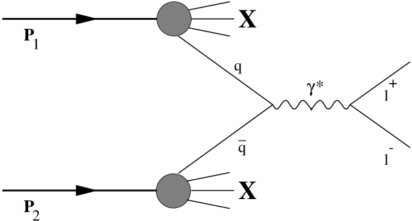
Figure 10: The DY process to leading order. Two hadrons collide and a quark from one hadron annihilates with an antiquark from the other hadron into a timelike photon with mass $M^{2}>0$. This photon decays into a lepton pair that can be detected.

We denote the mass of the spacelike photon by

$$M^{2}=q^{2}>0,$$ (116)

where $q^{\mu}$ is the four momentum of the virtual photon. The square of the center of mass energy of the colliding hadrons is

$$S=(P_{1}+P_{2})^{2},$$ (117)

where $P_{1}$ and $P_{2}$ are the four momenta of hadron $1$ and hadron $2$, respectively. A convenient variable to work with is Feynman $x_{F}$,

$$x_{F}=\frac{2p_{L}^{cm}}{\sqrt{S}}\approx x_{1}-x_{2}.$$ (118)

Here, $p_{L}^{cm}$ is the longitudinal momentum of the dilepton in the hadron-hadron center of mass frame and $x_{1}$ and $x_{2}$ are given by

$$x_{1}=\frac{2P_{2}\cdot q}{S}\quad,\quad x_{2}=\frac{2P_{1}\cdot q}{S}.$$ (119)

These variables have the meaning of the longitudinal momentum fractions of the quarks participating in the hard process. The quark $q$ in fig. 10 has longitudinal momentum $x_{1}P_{1}$ and the antiquark $x_{2}P_{2}$. It holds

$$x_{1}x_{2}=\frac{M^{2}}{S},$$ (120)

where the transverse momentum of the virtual photon is zero in the naive parton model and has been neglected. Another frequently used variable is

$$\tau=\frac{M^{2}}{S}.$$ (121)

Similar structure functions as in DIS can be introduced for the DY process, starting directly from the hadronic tensor,

$$W^{\mu\nu}=\int d^{4}x{\rm e}^{{\rm i}qx}\langle P_{1}P_{2}|J^{\mu}(x)J^{\nu}(0)|P_{1}P_{2}\rangle,$$ (122)

as we did in section 2.1. Since there are two hadrons involved in DY, there are more possible Lorentz structures than in DIS. One can define four independent structure functions for DY, rather than two in DIS. We do not pursue this approach in detail and refer only to the literature [114].

The partonic cross section for fig. 10 reads

$$\frac{d\widehat{\sigma}}{dM^{2}}=\frac{4\pi\alpha^{2}_{em}Z_{f}^{2}}{3N_{c}M^{2}}\delta(x_{1}x_{2}S-M^{2}).$$ (123)

The factor $N_{c}$, number of colors, appears in the denominator, because quark and antiquark must have the same color in order to annihilate. Embedding the partonic cross section into the hadronic environment yields

$$\frac{d\sigma}{dM^{2}}=\int_{0}^{1}dx_{1}dx_{2}\sum_{f}\left\{q_{f}(x_{1})\bar{q}_{f}(x_{2})+(1\leftrightarrow 2)\right\}\frac{d\widehat{\sigma}}{dM^{2}},$$ (124)

where $q_{f}(x_{1})$ is the probability to find a quark of flavor $f$ with longitudinal momentum fraction $x_{1}$ in hadron $a$ and $\bar{q}_{f}$ is the analog for antiquarks. The $\delta$-function in (123) allows to write the cross section in the scaling form

$$M^{2}\frac{d\sigma}{d\tau}=\frac{4\pi\alpha^{2}_{em}}{3N_{c}}\int_{0}^{1}dx_{1}\sum_{f}Z_{f}^{2}\left\{q_{f}(x_{1})\bar{q}_{f}(\tau/x_{1})+(1\leftrightarrow 2)\right\}.$$ (125)

The r. h. s. of (125) depends only on $\tau$ and not separately on $M^{2}$ and $S$.

The observation of this scaling property in experiment, see e. g.  [115, 116], confirms that the mechanism illustrated in fig. 10 is correct. There are however features of dilepton production which cannot be understood in the lowest order picture.

• Cross sections calculated straightforward from (125) are too small by a factor of $2-3$ compared to the measured value. This discrepancy is usually treated by introducing a so called $K$-factor. The $K$-factor is approximately independent of $M^{2}$, but it is process dependent.

• Large transverse photon momenta, of order few GeV, are observed in experiment. There are however no transverse momenta in the naive parton model. Phenomenologically, one can introduce a primordial momentum distribution of the quarks. One usually assumes a gaussian shape for this distribution, but the width necessary to describe what is observed in experiment is much larger than what one would expect from Fermi motion.

These problems can be overcome by taking into account the first order QCD correction, shown in fig. 11. The first row contains the virtual corrections to the quark propagator and to the vertex. The second row shows the so called annihilation process, where the quark or the antiquark radiates a gluon before it annihilates with a parton from the other hadron. Due to the radiation of the gluon, the quark acquires a transverse momentum. In this way, the pQCD correction provides the missing mechanism for the production of lepton pairs with large transverse momentum $p_{T}$. This explanation was suggested first in [118, 119, 120]. The last row displays the diagrams for the QCD Compton process, where a quark in one hadron picks up a gluon from the other hadron and radiates a photon. This mechanism is dominant at large $p_{T}$ [53].

Figure 11: Higher order QCD corrections to the DY process. The upper row contains virtual corrections. The diagrams for the annihilation process are shown in the middle, where the quark or the antiquark can radiate a gluon before the annihilation process. The QCD Compton process is depicted in the last row. Here, the projectile quark scatters off a gluon from the target and radiates a massive photon. The Compton process is the dominant contribution. These higher order corrections account for most of the K-factor and explain the occurance of large transverse momenta. The figure is taken from [117].

The graphs in fig. 11 contain of course divergencies. While the infrared divergencies cancel in the sum of virtual and real corrections, the collinear divergencies, which occur e. g. when the transverse momentum $p_{T}$ of the intermediate quark in the QCD Compton process goes to $0$, turn out to be identical to the divergencies observed in DIS, cf. section 2.2. Thus they can be absorbed into a redefinition of parton densities. For example, the QCD Compton process gives the additional contribution [119]

$$M^{2}\frac{d\sigma}{d\tau}\Bigg{|}_{C} = \frac{4\pi\alpha^{2}_{em}}{3N_{c}}\int_{0}^{1}\frac{dx_{1}}{x_{1}}\int_{0}^{1}\frac{dx_{2}}{x_{2}}\sum_{f}Z_{f}^{2}\left\{(q_{f}(x_{1})+q_{\bar{f}}(x_{1}))G(x_{2})+(1\leftrightarrow 2)\right\}$$ (126)

$$\times \Theta(x_{1}x_{2}-\tau)\frac{\alpha_{s}}{2\pi}P_{fG}\left(\frac{\tau}{x_{1}x_{2}}\right)\ln\left(\frac{M^{2}}{\kappa^{2}}\right)+\dots,$$

where $\Theta$ is the step function and $P_{fG}$ is given by (34). It was first noticed in [119], that the whole DY cross section, including (126) can be recasted in the form (125) by redefining the quark density,

$$q_{f}(x)\to q_{f}(x)+\frac{\alpha_{s}}{2\pi}\ln\left(\frac{M^{2}}{\kappa^{2}}\right)\int_{x}^{1}\frac{dy}{y}P_{fG}\left(\frac{x}{y}\right)G(y).$$ (127)

This is exactly what was done for DIS in section 2.2. Thus the redefined parton densities in DY obey the same renormalization group equation as the DIS parton densities, namely the DGLAP equations (38).

The first order correction solves most of the problems of the naive parton model. It explains how large $p_{T}$-dileptons are produced and account for almost all of the $K$-factor [117]. However, not all problems are solved by this correction. Since it is numerically large, one has to investigate how much higher order corrections change the result. Furthermore, the transverse momentum spectrum is even qualitatively not well described. The theoretical result agrees only at $p_{T}^{2}\sim M^{2}$ with the data and even diverges at $p_{T}\to 0$,

$$\frac{d\sigma}{dp_{T}^{2}}\sim\frac{\alpha_{s}(p_{T}^{2})}{p_{T}^{4}}$$ (128)

while the experimental result is of course finite. The reason for this behavior is that large logarithms $\ln({M^{2}}/{p_{T}^{2}})$ occur in higher order corrections and one has to resum all these terms. This is possible within pQCD [121, 122, 123], by a resummation of soft gluons radiated from the quark or the antiquark, respectively. The result indicates that one needs almost no intrinsic transverse momentum and practically all $p_{T}$ is generated perturbatively [124].

2.6 Light-cone approach to DY

Although cross sections are Lorentz invariant, the partonic interpretation of the microscopic process depends on the reference frame. We have seen this in section 2.3 for the case of DIS and similar considerations can be made for DY. It was pointed out by Kopeliovich [14] that in the target rest frame, DY dilepton production looks like bremsstrahlung, rather than parton annihilation. The space-time picture of the DY process in the target rest frame is illustrated in fig. 2. A quark (or an antiquark) from the projectile hadron radiates a virtual photon on impact on the target. The radiation can occur before or after the quark scatters off the target. Only the latter case is shown in fig. 2.

The cross section for radiation of a virtual photon from a quark after scattering on a proton, can be written in factorized light-cone form [14, 15, 16],

$$\frac{d\sigma(qp\to q\gamma^{*}p)}{d\ln\alpha}=\int d^{2}\rho\,|\Psi^{T,L}_{\gamma^{*}q}(\alpha,\rho)|^{2}\sigma_{q\bar{q}}(\alpha\rho),$$ (129)

similar to the DIS case (44). Here $\alpha$ is the longitudinal momentum fraction of the quark, carried away by the photon. The LC wavefunctions for DY can be written in the same form as in DIS (69),

$$\Psi^{T,L}_{\gamma^{*}q}(\alpha,\vec{\rho})=\frac{\sqrt{\alpha_{em}}}{2\pi}\left(\bar{\chi}_{q}\widehat{\cal O}_{\gamma^{*}q}^{T,L}\chi_{q}\right){\rm K}_{0}(\eta\rho).$$ (130)

Summation over quark helicities and polarizations of the photon is understood in (69). Here, the extension parameter

$$\eta^{2}=m_{f}^{2}\alpha^{2}+M^{2}\left(1-\alpha\right).$$ (131)

is the anolog of the extension parameter $\varepsilon$ (47) in DIS. As usual, the index $T$ stands for transverse photons and $L$ for longitudinal. The $\chi$ are again two component spinors, but the operators $\widehat{O}_{\gamma^{*}q}^{T,L}$ read now [16]

$$\widehat{\cal O}_{\gamma^{*}q}^{T} = {\rm i}m_{f}\alpha^{2}\vec{e}\cdot(\vec{n}\times\vec{\sigma})-{\rm i}(2-\alpha)(\vec{e}\cdot\vec{\nabla}_{\rho})+\alpha\vec{e}\cdot(\vec{\sigma}\times\vec{\nabla}_{\rho}),$$ (132)

$$\widehat{\cal O}_{\gamma^{*}q}^{L} = 2M(1-\alpha).$$ (133)

The two dimensional gradient $\vec{\nabla}_{\rho}$ acts on the transverse coordinate $\vec{\rho}$, $\vec{n}$ is the unit vector parallel to the momentum of the projectile quark and $\vec{\sigma}$ is the three vector of the Pauli spin-matrices. The LC wavefunctions for the transition $q\to\gamma^{*}q$ read explicitly for a given flavor of unit charge

$$|\Psi_{\gamma^{*}q}(\alpha,\rho)|^{2} = |\Psi^{T}_{\gamma^{*}q}(\alpha,\rho)|^{2}+|\Psi^{L}_{\gamma^{*}q}(\alpha,\rho)|^{2},$$ (134)

$$|\Psi^{T}_{\gamma^{*}q}(\alpha,\rho)|^{2} = \frac{\alpha_{em}}{\pi^{2}}\left\{m_{f}^{2}\alpha^{4}{\rm K}_{0}^{2}\left(\eta\rho\right)+\left[1+\left(1-\alpha\right)^{2}\right]\eta^{2}{\rm K}_{1}^{2}\left(\eta\rho\right)\right\},$$ (135)

$$|\Psi^{L}_{\gamma^{*}q}(\alpha,\rho)|^{2} = \frac{2\alpha_{em}}{\pi^{2}}M^{2}\left(1-\alpha\right)^{2}{\rm K}_{0}^{2}\left(\eta\rho\right).$$ (136)

Comparing (135) and (136) with their DIS counterparts (45) and (46) shows that the factor $N_{c}$ is no longer present in the $q\to\gamma^{*}q$ LC wavefunctions. This corresponds to the $N_{c}$ in the denominator of (123). Furthermore, we see that $|\Psi^{T}_{\gamma^{*}q}(\alpha,\rho)|^{2}$ has an extra factor of $2$, because in the DY process, one has to sum over the transverse polarizations of the photon, rather than average like in DIS.

For embedding the partonic cross section (129) into the hadronic environment, one has to note that the photon carries away the momentum fraction $x_{1}=(\sqrt{x_{F}^{2}+4\tau}+x_{F})/2$ from the projectile hadron. The hadronic cross section reads then

$$\frac{d\sigma}{dM^{2}dx_{F}} = \frac{\alpha_{em}}{6\pi M^{2}}\frac{x_{1}}{x_{1}+x_{2}}\int_{x_{1}}^{1}\frac{d\alpha}{\alpha^{2}}\sum_{f}Z_{f}^{2}\left\{q_{f}\left(\frac{x_{1}}{\alpha}\right)+q_{\bar{f}}\left(\frac{x_{1}}{\alpha}\right)\right\}\frac{d\sigma(qp\to q\gamma^{*}p)}{d\ln\alpha}$$ (138)

$$= \frac{\alpha_{em}}{6\pi M^{2}}\frac{1}{x_{1}+x_{2}}\int_{x_{1}}^{1}\frac{d\alpha}{\alpha}F_{2}^{p}\left(\frac{x_{1}}{\alpha}\right)\frac{d\sigma(qp\to q\gamma^{*}p)}{d\ln\alpha},$$

where the factor $\alpha_{em}/(6\pi M^{2})$ accounts for the decay of the photon into the lepton pair. Remarkably, the parton density of the projectile enters just in the combination $F_{2}^{p}$ (29), which is the structure function of the proton. Therefore we did not include the fractional quark charge $Z_{f}$ in the DY wavefunctions (135, 136). The structure function $F_{2}^{p}$ is needed at large values of $x_{Bj}$. We will employ the parametrization from [125] in our calculations, unless mentioned differently.

An interesting feature of the light-cone approach is the appearance of the dipole cross section in (129), although there is no physical $q\bar{q}$-dipole in fig. 2. The explanation is illustrated in fig. 12. The antiquark enters, when one takes the complex conjugate of the amplitude. The dipole cross section appears, because the quark is displaced in the impact parameter plane after radiation of the photon. If $\rho$ is the transverse separation between the quark and the photon, the $\gamma^{*}q$ fluctuation has a center of gravity in the transverse plane which coincides with the impact parameter of the parent quark. The transverse separation between the photon and the center of gravity is $(1-\alpha)\rho$ and the distance between the quark and the center of gravity is correspondingly $\alpha\rho$. A displacement in coordinate space corresponds to a phase factor in momentum space. The two graphs (a) and (b) in fig. 12 have the relative phase factor $\exp({\rm i}\alpha\vec{\rho}\cdot\vec{p}_{T})$, which produces the color screening factor $[1-\exp({\rm i}\alpha\vec{\rho}\cdot\vec{p}_{T})]$ in the dipole cross section (48). Therefore, the argument of the dipole cross section is $\alpha\rho$.

Figure 12: Two out of four contributions for the DY cross section. In the first row, the photon is radiated on both sides of the cut after the quark gluon vertex. The antiquark enters through the complex conjugate of the amplitude on the r.h.s. of the cut. The second row shows the interference term. The graphs in (a) and (b) have a relative phase factor $\exp({\rm i}\alpha\vec{\rho}\cdot\vec{p}_{T})$, where $p_{T}$ is the transverse momentum of the photon. This gives rise to the color screening factor in the dipole cross section (48) as explained in the text.

The physical interpretation of (129) is the same as for the DIS case, cf. section 2.3. The projectile quark is expanded in the interaction eigenstates (58). We keep only the first eigenstate,

$$|q\rangle=\sqrt{Z_{2}}|q_{bare}\rangle+c^{q}_{\gamma^{*}}|q\gamma^{*}\rangle+\dots,$$ (139)

where, $Z_{2}$ is the wavefunction renormalization constant for fermions. Different eigenstates scatter with different amplitudes off the target. This disturbs the coherence between the eigencomponents and the photon is freed. Since there is no real dipole in DY, we will not include a nonperturbative interaction, as it was done for DIS in section 2.3, but always use the perturbative LC wavefunctions (135, 136).

The light-cone approach to the DY process is applicable only at low $x_{2}$, because the dipole cross section takes only sea quarks generated from gluon splitting into account. Therefore, the dipole cross section is proportional to the target gluon density. The statement, whether a sea quark belongs to the target or to the projectile, is however frame dependent. If the projectile quark or antiquark becomes slow in the limit $\alpha\to 1$, in the infinite momentum frame, it can be interpreted in the infinite momentum frame as anti-seaquark or seaquark of the target which annihilates with the projectile parton. No annihilation with valence quarks from the target is taken into account. Note however that valence as well as sea parton distributions of the projectile are taken into account in the light-cone approach, if one employs a parametrization of the projectile structure function in (138). Therefore, the formulation of the DY process presented in this section is not fully symmetric between projectile and target.

It is also interesting to see that with the substitution

$$\alpha=\frac{1}{1+\widetilde{\alpha}}\quad,\quad\rho=\frac{\widetilde{\rho}}{\alpha},$$ (140)

the transverse DY cross section (138) can be rewritten as

$$\frac{d\sigma^{T}}{dM^{2}dx_{F}} = \frac{\alpha^{2}_{em}}{6\pi^{3}M^{2}}\frac{x_{1}}{x_{1}+x_{2}}\int^{\frac{1-x_{1}}{x_{1}}}_{0}d\widetilde{\alpha}\sum_{f}Z_{f}^{2}\frac{q_{f}(x_{1}(1+\widetilde{\alpha}))+q_{\bar{f}}(x_{1}(1+\widetilde{\alpha}))}{(1+\widetilde{\alpha})^{2}}$$ (141)

$$\times \int d^{2}\widetilde{\rho}\left\{\left[1+2\widetilde{\alpha}(1+\widetilde{\alpha})\right]\widetilde{\varepsilon}^{2}{\rm K}^{2}_{1}(\widetilde{\varepsilon}\widetilde{\rho})+m_{f}^{2}{\rm K}^{2}_{0}(\widetilde{\varepsilon}\widetilde{\rho})\right\}\sigma_{q\bar{q}}(\widetilde{\rho}),$$

and similarly for the longitudinal case, where $\widetilde{\varepsilon}=\widetilde{\alpha}(1+\widetilde{\alpha})M^{2}+m_{f}^{2}$ is the analog of the DIS extension parameter (47). One immediately recognizes the similarity with the $q\bar{q}$ wavefunction (45) in this equation. Indeed, the exact LC wavefunctions for DIS can be obtained by analytic continuation from timelike to spacelike region $M^{2}\to-Q^{2}$ and $\widetilde{\alpha}\to-\alpha$.

In the rewritten form (141), our expression for the DY cross section agrees with the result of Brodsky, Hebecker and Quack [15], where factorization in impact parameter space was considered. Note that the discussion of hard and soft contributions to DIS in section 2.3 immediately carries over to DY. Configurations with $\widetilde{\alpha}\to 0$ are the analog of the aligned jet configurations in DIS. Since $\widetilde{\alpha}=p_{q}^{\prime\,0}/q^{0}$ is the energy of the quark in the final state divided by the photon energy, large distances become important, when $\widetilde{\alpha}\to 0$ and $\alpha\to 1$, respectively. It appears however only one limiting case in DY, whereas in DIS (44), two extremely asymmetric cases allow for large distances.

For zero quark mass, the divergencies arising from the endpoints in the $\alpha$-integration, correspond to the logarithmic divergencies occuring in the standard approach, cf. sections 2.2 and 2.5, which were absorbed into the nonperturbative parton densities. A similar procedure can be performed in impact parameter space [15]. In the parton model, the differential DY cross section can be written as

$$\frac{d^{2}\sigma}{dx_{F}dM^{2}}=\frac{4\pi\alpha_{em}}{9M^{4}}\frac{x_{1}x_{2}}{x_{1}+x_{2}}\sum_{f}Z_{f}^{2}\left\{q_{f}(x_{1})\bar{q}_{f}(x_{2})+q_{f}(x_{2})\bar{q}_{f}(x_{1})\right\}.$$ (142)

The region $\widetilde{\alpha}\to 0$ is the DY analog of Bjorkens aligned jet configurations and gives a leading twist contribution to the transverse DY cross section. As explained above, a soft outgoing quark in the target rest frame can be regarded as part of the nonperturbative sea-antiquark distribution of the target in the infinite momentum frame. Neglecting the quark mass $m_{f}$, the divergent part of the integral (141) can be recasted into the form (142) and one can read of the quark and antiquark distributions of the target at low $x_{2}$. One find [15]

$$x_{2}q^{DY}_{f,\bar{f}}(x_{2})=\frac{3M^{2}}{8\pi^{4}}\int_{0}^{\Lambda}d\widetilde{\alpha}\int d^{2}\widetilde{\rho}\,\widetilde{\alpha}M^{2}{\rm K}^{2}_{1}(\widetilde{\varepsilon}\widetilde{\rho})\sigma_{q\bar{q}}(\widetilde{\rho}),$$ (143)

where $\Lambda\ll 1$ is a cutoff and the approximation $\widetilde{\varepsilon}\to\widetilde{\alpha}M^{2}$ for $\widetilde{\alpha}\to 0$ was used. On the other hand, in the parton model of DIS, one has

$$\frac{Q^{2}}{4\pi^{2}\alpha_{em}}\sigma^{\gamma^{*}p}_{T}=\sum_{f}Z_{f}^{2}\left\{q_{f}(x_{Bj})+\bar{q}_{f}(x_{Bj})\right\},$$ (144)

and one can again extract the divergent part of the integral (44) for the transverse cross section and read of the target parton distributions [15],

$$x_{Bj}q^{DIS}_{f,\bar{f}}(x_{Bj})=\frac{3Q^{2}}{8\pi^{4}}\int_{0}^{\Lambda}d\alpha\int d^{2}\rho\alpha Q^{2}{\rm K}^{2}_{1}(\varepsilon\rho)\sigma_{q\bar{q}}(\rho).$$ (145)

Note, that in DIS a slow quark ($\alpha\to 0$) seen in the target rest frame, can be interpreted as part of the sea-antiquark distribution of target in the infinite momentum frame. Obviously, the equations (143) and (145) are identical and therefore the DIS parton distribution is identical to the DY parton distribution. This manifestation of factorization in impact parameter space was first pointed out in [15].

The transverse momentum distribution of DY pairs can also be calculated in the light cone approach [16]. The differential cross section is given by the four-fold Fourier integral

$$\frac{d\sigma(qp\to q\gamma^{*}p)}{d\ln\alpha d^{2}p_{T}} = \frac{1}{(2\pi)^{2}}\int d^{2}\rho_{1}d^{2}\rho_{2}\,\exp[{\rm i}\vec{p}_{T}\cdot(\vec{\rho}_{1}-\vec{\rho}_{2})]\Psi^{*}_{\gamma^{*}q}(\alpha,\vec{\rho}_{1})\Psi_{\gamma^{*}q}(\alpha,\vec{\rho}_{2})$$ (146)

$$\times \frac{1}{2}\left\{\sigma_{q\bar{q}}(\alpha\rho_{1})+\sigma_{q\bar{q}}(\alpha\rho_{2})-\sigma_{q\bar{q}}(\alpha(\vec{\rho}_{1}-\vec{\rho}_{2}))\right\}.$$

after integrating this expression over $p_{T}$, one obviously recovers (129). The negative term in the curly brackets arises from the interference between the two graphs for bremsstrahlung. The expressions for the LC wavefunctions needed here are

$$\Psi^{*T}_{\gamma^{*}q}(\alpha,\vec{\rho}_{1})\Psi^{T}_{\gamma^{*}q}(\alpha,\vec{\rho}_{2}) = \frac{\alpha_{em}}{\pi^{2}}\Bigg{\{}m_{f}^{2}\alpha^{4}{\rm K}_{0}\left(\eta\rho_{1}\right){\rm K}_{0}\left(\eta\rho_{2}\right)$$ (147)

$$+ \left[1+\left(1-\alpha\right)^{2}\right]\eta^{2}\frac{\vec{\rho}_{1}\cdot\vec{\rho}_{2}}{\rho_{1}\rho_{2}}{\rm K}_{1}\left(\eta\rho_{1}\right){\rm K}_{1}\left(\eta\rho_{2}\right)\Bigg{\}},$$

$$\Psi^{*L}_{\gamma^{*}q}(\alpha,\vec{\rho}_{1})\Psi^{L}_{\gamma^{*}q}(\alpha,\vec{\rho}_{2}) = \frac{2\alpha_{em}}{\pi^{2}}M^{2}\left(1-\alpha\right)^{2}{\rm K}_{0}\left(\eta\rho_{1}\right){\rm K}_{0}\left(\eta\rho_{2}\right).$$ (148)

The hadronic cross section is then given by

$$\frac{d\sigma}{dM^{2}dx_{F}d^{2}p_{T}}=\frac{\alpha_{em}}{6\pi M^{2}}\frac{1}{x_{1}+x_{2}}\int_{x_{1}}^{1}\frac{d\alpha}{\alpha}F_{2}^{p}\left(\frac{x_{1}}{\alpha}\right)\frac{d\sigma(qp\to q\gamma^{*}p)}{d\ln\alpha d^{2}p_{T}},$$ (149)

in analogy to (138). Three of the four integrations in (146) can be performed analytically for arbitrary $\sigma_{q\bar{q}}$. This will be done in appendix A.1.

2.7 The dipole cross section

In this section we present a parametrization of the dipole cross section which is adjusted to DIS data and to total hadronic cross sections. In the preceding sections we have expressed the cross section for DIS and the DY-process at low $x$ in terms of the dipole cross section. Thus the dipole cross section is the crucial missing input one needs to perform a calculation that can be compared to experimental data. The dipole cross section is of interest not only for DIS and DY. Total hadronic cross sections, like for pion-proton scattering can also be written in terms of the dipole cross section. In this case, the pion wave-function in coordinate representation $\Psi_{\pi}(\rho)$, gives the probability to find a quark-antiquark pair with a given transverse separation inside the pion. If only the lowest Fock state is taken into account, the total cross section at c.m. energy $s$ can then be written as

$$\sigma_{\pi p}(s)=\int d^{2}\rho|\Psi_{\pi}(\rho)|^{2}\sigma_{q\bar{q}}(s,\rho),$$ (150)

in complete analogy to the DIS case. This is remarkable since hadronic cross sections are governed by nonperturbative long distance physics in contrast to DIS. Still, (150) is valid, because the decomposition into interaction eigenstates (58) is completely general and does not rely on perturbation theory.

The dipole cross section is largely unknown, only at small distances $\rho$ it can be expressed in terms of the gluon density (52). However, several parametrizations exist in the literature, describing the whole function $\sigma_{q\bar{q}}(\rho)$, without explicitly taking into account the QCD evolution of the gluon density. A very economical parametrization is provided by the saturation model of Golec-Biernat and Wüsthoff [80, 81],

$$\sigma_{q\bar{q}}(x,\rho)=\sigma_{0}\left[1-\exp\left(-\frac{\rho^{2}Q_{0}^{2}}{4(x/x_{0})^{\lambda}}\right)\right],$$ (151)

where $Q_{0}=1$ GeV and the three fitted parameters are $\sigma_{0}=23.03$ mb, $x_{0}=0.0003$, and $\lambda=0.288$. This dipole cross section vanishes $\propto\rho^{2}$ at small distances, as implied by color transparency and levels off exponetially at large separations, which reminds of eikonalization. The authors are able to fit all available HERA data with a quite low $\chi^{2}$ [80] and can furthermore also describe diffractive HERA data [81]. It is argued that saturation is necessary to obtain a nearly $Q^{2}$ independent ratio of the diffractive to the total cross section, which cannot be reproduced with a dipole cross section that rises quadratically up to infinity.

There is however no $x_{Bj}$ in hadron-hadron scattering and the appropriate variable to describe the energy dependence of the dipole cross section is $s$. This is different in DIS where the virtual photon scatters off pointlike constituents inside the proton and $x_{Bj}$ is the correct variable to use. Parametrizing the dipole cross section as function of $s$ will automatically lead to a violation of Bjorken scaling. This is easy to see, since $s\approx Q^{2}/x_{Bj}$. If the cross section is supposed to grow like a power of $s$, it will grow with approximately the same power in $Q^{2}$.

A two pomeron model of the dipole cross section as function of $s$, motivated from Regge phenomenology, was given in [82]. It was argued in [83] that the authors of [82] had to parametrize the dipole cross section as a function of $\rho^{2}s$, to get approximate Bjorken scaling. The ansatz of [82] can describe deep inelastic data up to $Q^{2}=60$ GeV², with $10$ parameters.

However, as can be seen from fig. 6, Bjorken scaling is quite strongly violated at low $x_{Bj}$. Since we have in mind to describe hadron-hadron scattering and DIS with the same dipole cross section, we write the dipole cross section as function of $s$. We are aware of the fact that our ansatz will fail at very large values of $Q^{2}$. Nevertheless, practically all physics which is interesting to us happens at quite small values of $Q^{2}<10$ GeV².

An ansatz inspired by the saturation model of [80, 81], was presented in [13]. It reads

$$\sigma_{q\bar{q}}(s,\rho)=\sigma_{0}(s)\left[1-\exp\left(-\frac{\rho^{2}}{r_{0}^{2}\left(s\right)}\right)\right],$$ (152)

with $r_{0}\left(s\right)=0.88(s/s_{0})^{-0.14}~{}{\rm fm}$, $s_{0}=1000~{}$GeV² and

$$\sigma_{0}(s)=\sigma_{tot}^{\pi p}(s)\left(1+\frac{3r_{0}^{2}\left(s\right)}{8\left<r^{2}_{ch}\right>_{\pi}}\right),$$ (153)

where $\sigma_{tot}^{\pi p}(s)=23.6(s/s_{0})^{0.08}~{}{\rm mb}$ and $\left<r^{2}_{ch}\right>_{\pi}=0.44~{}{\rm fm}^{2}$ is the pion charge radius. This cross section is proportional to $\rho^{2}$ for $\rho\to 0$, but flattens off at large $\rho$. The energy dependence correlates with $\rho$. At small $\rho$ the dipole cross section rises with a hard pomeron intercept, $0.36$, and at large separations it still depends with a soft pomeron intercept, $0.08$, on energy. This is different in (151), where the maximum value of the dipole cross section is independent of energy. We also mention that a value of $\sigma_{0}=23.03$ mb is too small to reproduce the pion-proton cross section. Note that the energy behavior of our parametrization is also conceptually different from Regge phenomenology, where the pomeron intercept has to be independent of the hadron. We think however, that the growth of the cross section with $s$ should depend on the typical distances involved and our ansatz smoothly interpolates between cross sections in hard QCD processes and soft hadronic scattering. The saturation scale $r_{0}(s)$ decreases with increasing $s$. This means that at very high $s$, only very small dipoles exhibit a hard pomeron behavior. At separations $\rho\gg r_{0}(s)$, the dipole cross section grows only slowly with energy. The ansatz (152) ensures that the dipole cross section is a monotonous function of $s$ and $\rho$. This is not the case for the parametrization of [82], which can decrease with increasing $\rho$.

The energy dependent saturation value of the parametrization (152) is chosen in such a way, that the pomeron part of the fit by Donnachie and Landshoff [126] is automatically reproduced, if one employs a gaussian pion wavefunction,

$$|\Psi_{\pi}(\rho)|^{2}=\frac{3}{8\pi\langle r^{2}_{ch}\rangle_{\pi}}\exp\left(-\frac{3\rho^{2}}{8\langle r^{2}_{ch}\rangle_{\pi}}\right).$$ (154)

To understand the factor of $3/8$, note that it has to hold

$$\int d^{2}\rho\,\rho^{2}\,|\Psi_{\pi}(\rho)|^{2}=\frac{2}{3}\cdot 2^{2}\langle r^{2}_{ch}\rangle_{\pi},$$ (155)

because $\vec{\rho}$ is only a two dimensional vector ($2/3$) and it has the meaning of a diameter, rather than a radius ($2^{2}$).

The dipole cross section (152) is however adjusted only by eye and no $\chi^{2}$ was calculated. Furthermore, it tends to overestimate $F_{2}$ at $Q^{2}>10$ GeV². We improve the parametrization (152) in several ways. First, we use the more recent fit by Cudell et al. [127],

$$\sigma_{\pi^{-}p}=26.2~{}{\rm mb}\,\left(\frac{s}{1~{}{\rm GeV}^{2}}\right)^{-0.357}+7.63~{}{\rm mb}\,\left(\frac{s}{1~{}{\rm GeV}^{2}}\right)^{-0.56}+12.08~{}{\rm mb}\,\left(\frac{s}{1~{}{\rm GeV}^{2}}\right)^{0.0933},$$ (156)

for $\sqrt{s}>9$ GeV². which has a slightly larger pomeron intercept and agrees better with experimental data than the old version by Donnachie and Landshoff [126]. A pomeron intercept larger than $0.08$ is also suggested by recent SELEX measurements [128], fig. 21. To improve the agreement with data, we multiplied (152) by a function that leads to a suppression at small value of $\rho$ and becomes $1$ at large $\rho$. We have tried several functions. Best agreement with HERA data is obtained with the parametrization

$$\sigma_{q\bar{q}}(s,\rho)=\sigma_{0}(s)\left[1-\exp\left(-\frac{\rho^{2}}{r_{0}^{2}\left(s\right)}\right)\right]\left[1-0.9\exp\left(-\frac{\rho^{2}}{r_{1}^{2}}\right)\right],$$ (157)

where

$$\sigma_{0}(s)=12.08~{}{\rm mb}\left(\frac{s}{1~{}{\rm GeV^{2}}}\right)^{0.0933}\left(1+\frac{3r_{0}^{2}\left(s\right)}{8\left<r^{2}_{ch}\right>_{\pi}}\right),$$ (158)

$$\left<r^{2}_{ch}\right>_{\pi}=0.44~{}{\rm fm}^{2},$$ (159)

$$r_{0}^{2}(s)=(2.19~{}{\rm fm})^{2}\left(\frac{s}{1~{}{\rm GeV^{2}}}\right)^{-0.34},$$ (160)

$$r_{1}=0.27~{}{\rm fm}.$$ (161)

Figure 13: The dipole cross section (157) for $\sqrt{s}=200$ GeV (HERA), solid line, and for $\sqrt{s}=1.4$ TeV (THERA), dashed line. The left figure shows the dipole cross section vs. $\rho$, while the figure on the right displays $\sigma_{q\bar{q}}(s,\rho)$ vs. $\rho^{2}$. At large separations, the dipole cross section becomes constant in $\rho$, but still grows slowly with energy. At small separations the dipole cross section depends quadratically on $\rho$.

Our result is depicted in fig. 13. The energy dependence of (157) is qualitatively the same as discussed for (152), because $r_{1}$ does not depend on $s$. In the left figure, we plotted the dipole cross section vs. $\rho$. One can see how the cross section increases from HERA to THERA energies. The figure on the right shows $\sigma_{q\bar{q}}(s,\rho)$ vs. $\rho^{2}$. At small separations, the dipole cross section increases quadratically with $\rho$.

We determined the $3$ parameters, $r_{1}$ and the two numbers in (160), using H1-data up to $Q^{2}=65$ GeV². We have tried to achieve good agreement with the same parameters for perturbative and nonperturbative wavefunctions. A comparison with data is presented in figs. 14-17. One observes that with perturbative LC wavefunctions, (45,46), the very low $Q^{2}$ data is not well reproduced. The agreement can be improved by introducing an unphysically small quark mass. This would however allow for arbitrarily large separations of the pair, at variance with confinement. We therefore fix the mass for $u$- and $d$-quarks at a typical inverse confinement radius,

$$m_{u,d}=200~{}{\rm MeV}.$$ (162)

We also include strange and charm quarks in our calculation,

$$m_{s}=350~{}{\rm MeV}\quad,\quad m_{c}=1.5~{}{\rm GeV}.$$ (163)

With these parameters, the lowest $\chi^{2}$ that can be obtained with perturbative wavefunctions is

$$\chi^{2}_{pt}({\rm H1},Q^{2}\leq 65~{}{\rm GeV}^{2})=523/233~{}{\rm d.o.f.}$$ (164)

Statistical and systematic errors are added in quadrature. However, the dashed curves still make a reasonable impression at not too high $Q^{2}$, when one looks at figs. 14-17. We will therefore perform all our calculations with perturbative wavefunctions, too. Better agreement is obtained with the nonperturbative wavefunctions, (2.3,78), which describe the data especially well at low $Q^{2}$. We obtain

$$\chi^{2}_{npt}({\rm H1},Q^{2}\leq 10~{}{\rm GeV}^{2}) = 86.4/100~{}{\rm d.o.f},$$ (165)

$$\chi^{2}_{npt}({\rm H1},Q^{2}\leq 30~{}{\rm GeV}^{2}) = 214/182~{}{\rm d.o.f}.$$ (166)

For the nonperturbative wavefunctions, we fix the quark masses at $m_{u}=m_{d}=10$ MeV, $m_{s}=150$ MeV and $m_{c}=1.5$ GeV. We have also plotted the result of our calculation for very high virtualities $Q^{2}=2000$ GeV², see figs. 15-16. The parametrization (157) overshoots the data at large $Q^{2}$.

Figure 14: The points show H1 data [130]-[133] for the proton structure function $F_{2}$ vs. $s$. Only statistical errors are shown. The solid curves are calculated with the parametrization (157) of the dipole cross section and with the nonperturbative LC wavefunctions (2.3,78). The dashed curves are the same but calculated with the perturbative LC wavefunctions (45,46). The parameters in (157) are adjusted to this set of data. See text for more details.

Figure 15: The same as fig. 14. The points shown here are not used to determine the parameters in (157).

Figure 16: The same as fig. 14 but the points are from ZEUS [61, 62, 134]-[137]. These points are not used to determine the parameters in (157).

Figure 17: The same as fig. 14 but the points are from ZEUS [61, 62, 134]-[137]. These points are not used to determine the parameters in (157).

To see in more detail, how the nonperturbative interaction modifies the LC wavefunctions and which distances contribute to $F_{2}$, we calculate the following three quantities. First, we integrate the LC wavefunctions over the longitudinal momentum fraction $\alpha$ and over the angle,

$$A_{0}(\rho)=\frac{2\pi\rho}{\alpha_{em}}\int_{0}^{1}d\alpha|\Psi^{T,L}_{q\bar{q}}(\alpha,\rho)|^{2}.$$ (167)

The result is shown in fig. 18. The results for our calculation of the wavefunctions integrated over $\alpha$ and angle weighted with the dipole cross section,

$$A_{1}(\rho)=\frac{2\pi\rho}{\alpha_{em}}\sigma_{q\bar{q}}(s,\rho)\int_{0}^{1}d\alpha|\Psi^{T,L}_{q\bar{q}}(\alpha,\rho)|^{2},$$ (168)

can be seen in fig. 19. This quantity is important for the structure function $F_{2}$. Finally, we weight the integral with $\sigma^{2}_{q\bar{q}}(s,\rho)$

$$A_{2}(\rho)=\frac{2\pi\rho}{\alpha_{em}}\sigma_{q\bar{q}}^{2}(s,\rho)\int_{0}^{1}d\alpha|\Psi^{T,L}_{q\bar{q}}(\alpha,\rho)|^{2},$$ (169)

which is important for diffraction. The result is depicted in fig. 20. In all three cases, the factor $2\pi\rho$ arises from the area element. It has to be included, if one wants to get a correct impression of the distances contributing to $F_{2}$. For convenience, we divide $A_{0}$–$A_{2}$ by the fine structure constant $\alpha_{em}$. All calculations are done at $\sqrt{s}=200$ GeV² and for two values of $Q^{2}$, namely for $Q^{2}=0.5$ GeV² and for $Q^{2}=10$ GeV².

Figure 18: The LC wavefunctions integrated over $\alpha$, (167), at $\sqrt{s}=200$ GeV. The solid curves are calculated with the nonperturbative wavefunctions, (2.3,78), while the dashed curves are calculated with the perturbative ones, (45,46). The lower two curves (at large $\rho$) are for $Q^{2}=10$ GeV² and the upper ones for $Q^{2}=0.5$ GeV².

It is hard to see in fig. 18, how the nonperturbative interaction modifies the transverse LC wavefunctions. Even at $Q^{2}=0.5$ GeV², the curves are almost identical. The transverse part diverges $\propto 1/\rho$ at $\rho\to 0$. The wavefunction is not normalizable. The curves rapidly decay as $\rho$ becomes larger, cf. (62). The situation is different in the longitudinal case. Here, $A_{0}$ goes to $0$ at $\rho\to 0$. The longitudinal wavefunction is square integrable. At high $Q^{2}$ the integral $A_{0}$ has a peak at small $\rho\approx 1/Q$ and then decreases exponentially. At low virtuality, this peak is much less pronounced and $A_{0}$ has quite a long tail into the large distance region. Somewhat surprisingly, the longitudinal LC wavefunctions are stronger affected by the nonperturbative interaction at low $Q^{2}$ than the transverse. At $Q^{2}=10$ GeV², no effect of the nonperturbative interaction is visible any more.

Figure 19: The LC wavefunctions integrated over $\alpha$ and weighted with $\sigma_{q\bar{q}}(s,\rho)$, (168), at $\sqrt{s}=200$ GeV. See fig. 18 for more explanations.

The quantity $A_{1}$ displayed in fig. 19 integrated over $\rho$ is nothing but the structure function $F_{2}$, up to a factor $Q^{2}/(4\pi^{2})$. The region of small $\rho$ is suppressed compared to fig. 18, because of an extra factor $\rho^{2}$ from the dipole cross section. Therefore, larger distances as one would expect contribute. Both, for low and high $Q^{2}$, the curves have a long tail into the large distance domain. Again, there is practically no influence of the nonperturbative interaction at high virtuality, but at low $Q^{2}$ and large $\rho$, the perturbative part is slightly suppressed compared to the nonperturbative. This means that our choice of the quark mass, squeezes the wavepacket somewhat more than the interaction. This can also be seen in figs. 14-17, where the perturbatively calculated curve is always below the nonperturbative. At very high $Q^{2}$, the curves become indistinguishable. We see again, that the longitudinal part is more strongly influenced by the interaction, than the transverse. Note also, that the longitudinal part is much smaller than the transverse, namely of order 20%.

Figure 20: The LC wavefunctions integrated over $\alpha$ and weighted with $\sigma^{2}_{q\bar{q}}(s,\rho)$, (169), at $\sqrt{s}=200$ GeV. See fig. 18 for more explanations.

We also plot the $\alpha$-integrated LC wavefunction, weighted with $\sigma^{2}_{q\bar{q}}(s,\rho)$. In fig. 20, we see that the small distance region is suppressed by an additional factor $\rho^{4}$, compared to fig. 18. Small distances play numerically no role, if one would integrate $A_{2}$ over $\rho$. This illustrates our discussion in section 2.4, where we argued that diffraction is dominated by soft physics, despite the large virtuality.

Figure 21: The points show the world data [129] for the $\pi^{-}p$ total cross section. The point at $\sqrt{s}\approx 35$ GeV is from the SELEX collaboration [128]. Only statistical errors are shown. The solid curve is calculated with the dipole cross section (157), while the dashed curve is the fit (156) from [127].

While the original parametrization of the dipole cross section from [13] reproduced identically the pomeron part of the Donnachie-Landshoff fit, the improved parametrization (157) does not have this property. We therefore check, how well we can reproduce the total $\pi^{-}p$ cross section with the wavefunction (154). Of course we have to add the reggeon exchange contribution from (156), since the dipole cross section describes only the pomeron part. The result is shown in fig. 21. We see that the cross section is not identically reproduced, as could have been expected. Our result is slightly smaller than the fit (156), because we multiplied the old parametrization (152) with a function that is always smaller than $1$. Nevertheless, the pion-proton cross section is reasonably well reproduced. The cross section calculated from our parametrization (157) grows with the same power of $s$ at high energy. One gets the impression from fig. 21 that the data grow even faster. At present, there is however no data available at higher energies than $\sqrt{s}=35$.

Figure 22: The points represent the measured DY cross section from [138]. Only statistical errors are shown. The curves are calculated with the dipole cross section (157) without any further fitting procedure. In order to make $x_{2}$ small, $x_{F}$ has to be large. In these two figures $0.01\leq x_{2}\leq 0.1$.

Figure 23: The transverse momentum distribution for DY pairs calculated from (149) with the dipole cross section (157).

We can now proceed and investigate how well our parametrization describes DY data. The light-cone approach is applicable only at low $x_{2}$, because it neglects valence quarks in the target. At present, there are however not many data for DY cross sections at low $x_{2}=(\sqrt{x_{F}^{2}+4\tau}-x_{F})/2$ or at large $x_{F}$, respectively. Only the data at the two largest values of $x_{F}$ from the E772 collaboration, correspond to values of $0.01\leq x_{2}\leq 0.1$. The result of our calculation, using (138), is shown in fig. 22. Although the data scatter a lot, one observes that the $M$ dependence is only approximately reproduced. We believe that this can be improved by modifying the dipole cross section. Remarkable is also that the absolute magnitude of the cross section is quite well reproduced, without introducing a $K$-factor. Indeed, we believe that it is not legitimate to use a $K$ factor in our approach, since the dipole cross section is supposed to parametrize all higher order corrections.

Furthermore, we also calculate the transverse momentum distribution of DY dilepton pairs from (149). The result is depicted in fig. 23. The DY cross section is finite at $p_{T}=0$, in contrast to the result of first order pQCD. We do not compare to data in fig. 23, because all available data are integrated over $x_{F}$ and are therefore contaminated by valence quark contributions. An extraction of the low-$x$ part of the transverse momentum distribution is in progress [139]. Note however, that the differential cross section is usually parametrized as [140, 116]

$$\frac{d\sigma}{dp_{T}^{2}}\propto\frac{1}{[1+(p_{T}/p_{0})^{2}]^{6}},$$ (170)

while our result decays much weaker and behaves approximately like

$$\propto\frac{1}{[1+(p_{T}/1~{}{\rm GeV})^{2}]^{2}}.$$ (171)

The behavior $\propto p_{T}^{4}$ is expected from pQCD at large $p_{T}^{2}>M^{2}$ and the finiteness at $p_{T}\to 0$ looks encouraging. It is at present not clear to us, whether a modified dipole cross section could reproduce the familiar shape (170), or whether the resummation of soft gluon radiation from the projectile quark requires additional modifications of the approach.

To summarize, our parametrization reproduces well the proton structure function $F_{2}$ from the lowest values of $Q^{2}\approx 0.1$ GeV² up to $Q^{2}\approx 30$ GeV², although it does not respect Bjorken scaling. The low $Q^{2}$ data is much better described if one employs the nonperturbative wavefunctions. Also at $Q^{2}>30$ GeV², the data is quite well reproduced if one looks at the plot only by eye. Since we have parametrized the dipole cross section as function of $s$, rather than $x_{Bj}$, we can also calculate total meson-proton cross sections, given an appropriate meson wavefunction. The total $\pi^{-}p$ cross section is reasonably well reproduced and also the few available DY data can be described without invoking a $K$-factor. Only the DY transverse momentum distribution looks different from what one would expect. At present, all data on the transverse momentum distribution is however integrated over $x_{F}$, making a comparison with calculations impossible. The differential cross section could give much more detailed information about the dipole cross section than the presently availabe total cross sections. Certainly (157) is not the final answer and has to be improved further and compared to more data. Especially diffractive DIS data which are more sensitive to the large distance region have not been taken into account so far. We will however compare our predictions for shadowing with data and nuclear shadowing is closely related to diffraction, as will be explained in the following section.

3 Nuclear shadowing in DIS and for DY

The typical energy and momentum scales in nuclear physics are much lower than the virtualities reaches in DIS. One could therefore expect that using nuclei instead of protons as target would only increase the cross section. There are however very pronounced nuclear effects in DIS. At intermediate values of $x_{Bj}$ one observes a suppression of the structure function ratio, fig. 24, known as the EMC effect [11]. This effect was unexpectedly discovered at CERN. It is described theoretically in terms of new degrees of freedom in nucleus, i.e. others than nucleons, see review [141]. We do not discuss the EMC effect any further and turn our attention to lower values of $x_{Bj}$. After a small enhancement in the region of $x_{Bj}\approx 0.1$, which is called antishadowing, one reaches the shadowing region, where $\sigma^{\gamma^{*}A}<A\sigma^{\gamma^{*}p}$ ($A$ is the nuclear mass number), i.e. a considerable depletion of the nuclear structure function is observed. During the last decade, nuclear shadowing has been measured at CERN (EMC, NMC), at Fermilab (E665) and recently also at DESY (HERMES). Values of $x_{Bj}<0.001$ can be reached, but most of the data are at higher values.

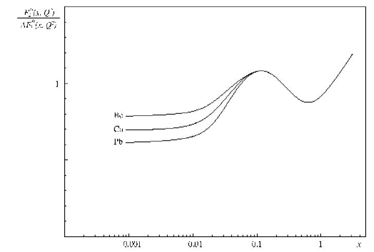
Figure 24: Schematic plot of nuclear effects in the ratio of the structure functions $F_{2}^{A}$ of a nucleus and the proton structure function $F_{2}^{N}$ vs. $x=x_{Bj}$. The suppression, $F_{2}^{A}/AF_{2}^{N}<1$, at $x_{Bj}<0.1$ is called nuclear shadowing. See text for more details. The figure is taken from [142].

After the pioneering work of Gribov [8], where shadowing arises from the interaction of virtual photons at the surface of the nucleus, this effect was not unexpected. Nuclear shadowing is of high theoretical interest, because it can be understood in terms of the fundamental degrees of freedom of QCD, quarks and gluons. In the preceding sections the ground for an investigation of nuclear shadowing in terms of the color dipole picture was prepared. In this part of the work, an improved version of the Glauber-Gribov theory is developed, which includes the nuclear form factor in the usual Glauber series. The interplay of multiple scattering and coherence are discussed in detail.

3.1 Shadowing and Diffraction

The partonic interpretation of shadowing depends on the reference frame. In the infinite momentum frame of the target, shadowing is due to parton fusion [143] - [146], which leads to a reduction of the parton density at low $x_{Bj}$. This can be understood intuitively in the following way [147]: In DIS a picture of the microscopic substructure of the target is taken. However, this cannot be done in an infinitely short time. The uncertainty relation tells us that the time needed increases as $x_{Bj}$ becomes small. This can be seen from the energy denominator in (43) on page 43. More precisely, the role of time is played by the logarithm of $x_{Bj}$, as can be seen from the double leading log DGLAP equation,

$$\frac{\partial^{2}x_{Bj}G(x_{Bj},Q^{2})}{\partial\ln(1/x_{Bj})\partial\ln Q^{2}}=\frac{N_{c}\alpha_{s}}{\pi}x_{Bj}G(x_{Bj},Q^{2}).$$ (172)

For fixed strong coupling constant $\alpha_{s}$, the solution behaves asymptotically like (39). While a fast moving nucleus is contracted to a pancake shape, the cloud of partons with very small momentum fraction is much less contracted and parton clouds from different nucleons will overlap. As the density becomes higher and higher with decreasing $x_{Bj}$, the partons start to feel the neighborhood of other partons and fusion processes like $GG\to G$ and $GG\to q\bar{q}$ will occur. These fusion processes reduce the parton density in a nucleus compared to a free nucleon.

A very intuitive picture arises in the rest frame of the nucleus, where the same phenomenon looks like nuclear shadowing of hadronic fluctuations of the virtual photon [12, 71, 72],[148] - [154]. Shadowing occurs, because of multiple scattering of the hadronic fluctuation inside the target. The nucleons at the surface of the nucleus cast a shadow on the inner nucleons, which then have less chances to interact with the photon. Multiple scattering at high energies is commonly described in the optical model of Glauber-Gribov theory. The basics of this approach have been formulated a long time ago by Glauber [7] within nonrelativistic quantum mechanics. The optical model is usually derived in eikonal approximation with the assumption that the phases obtained in different scatterings are additive. Of course, one would like to have a connection to quantum field theory and the Feynman diagram technique, which allows to include relativistic kinematics. This has been elaborated by Gribov [8]. However, the relation between Glauber theory and Feynman diagrams has been fully explored only for the double scattering term. The theory has been developed by many authors since then. In [155], Gribovs approach is generalized to non forward scattering and an expression is obtained which also includes inelastic transitions. For a discussion of Glauber-Gribov theory in the context of Regge phenomenology see for instance [156].

We give a short summary of the Glauber-Gribov theory, following [155]. For simplicity, only forward scattering is considered, although the approach can be generalized to include also small momentum transfers. All correlations between the nucleons will be neglected in the following. The total amplitude for scattering off a nucleus is written as a sum over $n$-fold scattering amplitudes.

$$F(s)=\sum_{n=1}^{A}F^{(n)}(s),$$ (173)

where $s$ is the photon-nucleon c.m. energy squared and $F^{(n)}(s)$ is the amplitude for an $n$-fold scattering. It can be written as an integral over impact parameter ($b$) space and over the longitudinal coordinates $z_{i}$ of the scatterings,

$$F^{(n)}(s) = \left(\frac{{\rm i}}{K}\right)^{n-1}\int d^{2}b\int\limits_{-\infty}^{\infty}dz_{1}\rho_{A}(b,z_{1})\int\limits_{z_{1}}^{\infty}dz_{2}\rho_{A}(b,z_{2})\dots\int\limits_{z_{n-1}}^{\infty}dz_{n}\rho_{A}(b,z_{n})$$ (174)

$$\times \sum_{\{h\}}f_{\gamma^{*}\to h_{1}}e^{-{\rm i}q_{L\gamma^{*}\to h_{1}}(z_{2}-z_{1})}f_{h_{1}\to h_{2}}e^{-{\rm i}q_{Lh_{1}\to h_{2}}(z_{2}-z_{3})}\dots f_{h_{n-1}\to\gamma^{*}}.$$

Here, $K\approx 2s$ is the flux factor. The expression (174) is illustrated in fig. 25. The nuclear density $\rho_{A}$, which is normalized to $A$, enters after integration over the wavefunction of the nucleus, neglecting correlations. It is assumed that the impact parameter $b$ does not change in a collision. The limits of the integrations over the longitudinal coordinates $z_{i}$ originate from the condition that the $(i+1)$th collision has to take place after the $i$th one. After the first collision, the virtual photon converts into a multiparticle hadronic state $h_{1}$. The amplitude for this process is denoted by $f_{\gamma^{*}\to h_{1}}$. Furthermore, the longitudinal momentum transfer $q_{L\gamma^{*}\to h_{1}}$ appears as an oscillating phase factor for each intermediate state. One has

$$q_{L\gamma^{*}\to h_{1}}=\frac{Q^{2}+M_{h_{1}}^{2}}{2\nu},$$ (175)

where $M_{h_{1}}$ is the invariant mass of the hadronic state $h_{1}$. Finally one has to sum over all states $h_{i}$ that can be reached by multiple scattering. According to the optical theorem, the total cross section is then given by

$$\sigma^{\gamma^{*}A}(s)=\frac{2F(s)}{K}.$$ (176)

Figure 25: Illustration of the $n$-fold scattering amplitude $F^{(n)}(s)$ (174) with intermediate hadronic states $1\dots n-1$. The upper part of the figure corresponds to the photon, which converts in different hadronic states due to multiple rescattering. The lower part corresponds the nucleus, where each line represents a nucleon. The amplitude for the transition $i\to j$ is denoted by $f_{j}$ in this figure.

Straightforward calculations with (174) are however not possible, because the intermediate states which can occur in an $n$-fold scattering are not known. Therefore, one is forced to introduce additional approximations. The idea to represent the virtual photon as superposition of hadrons with the same quantum numbers, namely vector mesons, leads to (generalized) vector dominance model (G)VDM [8, 103]. The advantage of this approach is that the masses of vector mesons are well defined, in contrast to the mass of a $q\bar{q}$ dipole in the mixed representation. The masses of the intermediate states have to be known, since they enter the longitudinal momentum transfers $q_{L}$. On the other hand it is not known, how to calculate scattering amplitudes, higher than the double scattering term, because vector mesons are no eigenstates of the interaction. A possible prescription would be to omit all off diagonal transitions which is called the diagonal approximation. Note that in the VDM, which is the diagonal approximation of the GVDM, one has to choose a vector meson-nucleon cross section that behaves as $\sigma_{Vp}\propto 1/M^{2}_{V}$, where $M_{V}$ is the mass of the vector meson, in order to reproduce the Bjorken scaling of the proton structure function. With a nearly constant $\sigma_{Vp}$, $F_{2}^{p}$ would increase linearly with $Q^{2}$. However, with such a fast decreasing meson-nucleon cross section, it turns out that nuclear shadowing is a higher twist effect. It was indeed believed for quite a long time that shadowing vanishes at large $Q^{2}$, until it was shown experimentally that this is not the case [2]. This phenomenon is sometimes called the Gribov paradox [157]. The solution is that one also has to take into account off-diagonal transitions, which correspond to diffraction dissociation. These off-diagonal transitions interfere destructively with the diagonal ones and one can reproduce the Bjorken scaling with an $M_{V}$ independent $\sigma_{Vp}$ [158]. The diagonal VDM is applicable only at low $Q^{2}<1$ GeV², where the proton structure function indeed rises approximately linearly, see fig. 6.

The close connection between shadowing and diffraction becomes most transparent in the formula derived by Karmanov and Kondratyuk [159]. In the double scattering approximation, the shadowing correction can be related to the diffraction dissociation spectrum, integrated over the mass,

$${\sigma^{\gamma^{*}A}} \approx A\sigma^{\gamma^{*}p}-{8\pi}\,\int d^{2}b\int\limits_{-\infty}^{\infty}dz_{1}\rho_{A}(b,z_{1})\int\limits_{z_{1}}^{\infty}dz_{2}\rho_{A}(b,z_{2})$$ (177)

$$\qquad\times\int dM^{2}_{X}\,\left.\frac{d\sigma(\gamma^{*}N\to XN)}{dM^{2}_{X}\,dt}\right|_{t\to 0}\cos\left(-{\rm i}\frac{Q^{2}+M_{X}^{2}}{2\nu}(z_{2}-z_{1})\right)$$

$$= A\sigma^{\gamma^{*}p}-{4\pi}\,\int d^{2}b\int dM^{2}_{X}\,\left.\frac{d\sigma(\gamma^{*}N\to XN)}{dM^{2}_{X}\,dt}\right|_{t\to 0}F_{A}^{2}(l_{c},b).$$ (178)

Note that the kinematical limit for $t$ is slightly larger than zero. This result is easily obtained from (174), when one neglects the small real part of the scattering amplitude $F(s)$. Here

$$F_{A}^{2}(l_{c},b)=\left|\int\limits_{-\infty}^{\infty}dz\rho_{A}(b,z){\rm e}^{{\rm i}z/l_{c}}\right|^{2}$$ (179)

is the formfactor of the nucleus. Again the coherence length

$$l_{c}=\frac{2\nu}{Q^{2}+M_{X}^{2}}$$ (180)

emerges. This length is of course already present in (174). The Karmanov-Kondratyuk equation is illustrated in fig. 26. The first term in (177) is the single scattering term, which is proportional to $A$. The second term represents the double scattering contribution and is responsible for shadowing. To model the influence of higher order rescattering terms, the shadowing correction is often multiplied by the term

$$\exp\left(-\frac{\sigma_{eff}}{2}\int dz\rho_{A}(b,z)\right),$$ (181)

with the effective absorption cross section $\sigma_{eff}\sim 20$ mb for quark shadowing. Note that at very high energies, the coherence length becomes infinite and the oscillating exponential in the nuclear form factor is practically unity which corresponds to maximum shadowing. Of course, the shadowing term still grows with energy, because of the diffractive cross section. As the energy becomes lower, the exponential oscillates more and more rapidly and the shadowing correction vanishes. This observation makes the importance of $l_{c}$ very clear.

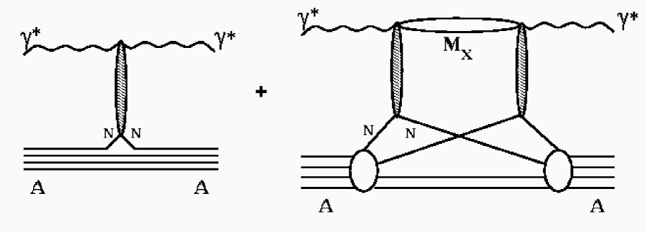
Figure 26: Illustration of the Karmanov-Kondratyuk formula (177). The left figure shows the single scattering contribution to DIS off nuclei. The double scattering term, shown on the right, gives the driving contribution to nuclear shadowing. It scales like $A^{\frac{4}{3}}$.

A simple estimate that demonstrates the relation between shadowing and diffraction is performed in [160], see also [12]. In [160], an infinite coherence length is assumed and the diffractive cross section is parametrized in the way,

$$\int dM^{2}_{X}\,\left.\frac{d\sigma(\gamma^{*}N\to XN)}{dM^{2}_{X}\,dt}\right|_{t\to 0}=B\sigma^{DD}_{\gamma^{*}p}.$$ (182)

The diffractive cross section $\sigma^{DD}_{\gamma^{*}p}\approx 0.1\sigma^{\gamma^{*}p}$ makes about 10% of the total cross section and the slope parameter which describes the $t$-dependence of diffraction is adjusted to $B\approx 8$ GeV^-2. Although no higher order scattering terms are taken into account, the authors of [160] obtain good agreement with experimental data at very low $x_{Bj}$. This analysis confirms the physical picture that shadowing in DIS is governed by coherent interaction of diffractively produced states in the nucleus, fig. 26.

From this discussion, two fundamental requirements emerge, which have to be fulfilled for shadowing.

• The mean free path of the hadronic fluctuation is long enough to have multiple scatterings. More quantitatively it must hold

  $$\frac{1}{\rho_{A}\sigma_{eff}}<R_{A},$$ (183)

  where $R_{A}$ is the nuclear radius.

• The coherence length $l_{c}$ has to be bigger than the mean inter-nucleon distance, $l_{c}>2$ fm. This condition ensures that the virtual photon coherently scatters off the nucleons.

One can also estimate, which masses $M_{X}$ can contribute to shadowing. Note that since

$$\frac{d\sigma(\gamma^{*}N\to XN)}{dM^{2}_{X}\,dt}\Big{|}_{t\to 0}\propto\frac{1}{M_{X}^{2}}$$ (184)

for large masses, one formally has to integrate the spectrum up to the kinematical limit. However, due to coherence length effects, large masses cannot contribute to shadowing. This can be seen in the following way. The coherence length can be written as

$$l_{c}=\frac{\beta}{m_{N}x_{Bj}}=\frac{1}{m_{N}x_{\cal P}}$$ (185)

with

$$\beta=\frac{Q^{2}}{Q^{2}+M_{X}^{2}}.$$ (186)

One finds from the second condition that only masses

$$M_{X}^{2}<0.1\,s$$ (187)

are relevant for shadowing. Note that this quantity can become much larger than $Q^{2}$ at low $x_{Bj}$. It is however small compared to $s$.

In the VDM and for the Karmanov-Kondratyuk formula, the multiple scattering amplitude (174) is evaluated in a hadronic basis. The disadvantage of using this basis is that one cannot calculate higher order scattering terms in an unambiguous way. We can however make use of our knowledge of the interaction eigenstates, namely partonic configurations frozen in impact parameter space. No off-diagonal transitions occur in this basis. One encounters however another severe problem, the mass of the eigenstates, which one has to know for the coherence length, is undefined in the mixed representation and one cannot give an explicit expression for the scattering amplitude. Only in the limit $l_{c}\to\infty$, it is possible to resum the whole multiple scattering series [155] in an eikonal-formula,

$$\sigma^{\gamma^{*}A} = 2\int d^{2}b\int_{0}^{1}d\alpha\int d^{2}\rho\left|\Psi(\alpha,\rho)_{q\bar{q}}\right|^{2}\left(1-\exp\left(-\frac{\sigma_{q\bar{q}}(s,\rho)}{2}T(b)\right)\right)$$ (188)

$$+ 2\int d^{2}b\int_{0}^{1}d\alpha\int\frac{d\alpha_{G}}{\alpha_{G}}\int d^{2}\rho_{1}d^{2}\rho_{2}\left|\Psi_{q\bar{q}G}(\alpha,\alpha_{G},\vec{\rho}_{1},\vec{\rho}_{2})\right|^{2}$$

$$\qquad\qquad\times\left(1-\exp\left(-\frac{\sigma_{q\bar{q}G}(s,\vec{\rho}_{1},\vec{\rho}_{2})}{2}T(b)\right)\right).$$

Summation over photon polarizations is understood. The nuclear thickness function $T(b)=\int_{-\infty}^{\infty}dz\,\rho_{A}(b,z)$ is the integral of nuclear density over longitudinal coordinate $z$ and depends on the impact parameter $b$. The light-cone wavefunctions are given by (45) and (46) on page 45 for the free case and by (2.3) and (78) on page 2.3 including the nonperturbative interaction. The LC wavefunction for the gluonic component is given by (115) on page 115. The cross section for the three body system $q\bar{q}G$ (108) can be expressed in terms of the dipole cross section. In the following more quantitative discussion, the $q\bar{q}G$-term is dropped and for the $q\bar{q}$-part the shorthand notation

$$\sigma^{\gamma^{*}A}=\left<2\int d^{2}b\left(1-\exp\left(-\frac{\sigma_{q\bar{q}}(s,\rho)}{2}T(b)\right)\right)\right>$$ (189)

is introduced. The condition $l_{c}\gg R_{A}$ insures that the $r$ does not vary during propagation through the nucleus (Lorentz time dilation) and one can apply the eikonal approximation. Note that the averaging of the whole exponential in (189) makes this expression different from the Glauber eikonal approximation where $\sigma_{q\bar{q}}(s,\rho)$ is averaged in the exponent,

$$2\int d^{2}b\left(1-\exp\left(-\frac{\sigma^{\gamma^{*}p}}{2}T(b)\right)\right).$$ (190)

The difference is known as Gribov’s inelastic corrections [8]. In the case of DIS the Glauber approximation does not make sense and the whole cross section is due to the inelastic shadowing. Indeed, $\sigma^{\gamma^{*}p}$ is at most of order $100$ $\mu$b, for real photons, which corresponds to a mean free path in nuclear matter of $l_{f}\approx 600$ fm. This means that the bare photon does practically not interact and therefore no multiple scattering can occur. The photon interacts only via its hadronic components.

The condition $l_{c}\gg R_{A}$ is however not fulfilled in most of the experiments. Only for the lowest values of $x_{Bj}$ in the E665 experiment, this condition is met. For the case $l_{c}\sim R_{A}$, one has to take into account the nuclear form factor, i.e. the variation of $\rho$ during the propagation of the $q\bar{q}$ fluctuation through the nucleus. This can be done for the $q\bar{q}$-component of the photon and in double scattering approximation [153, 154],

$$\sigma^{\gamma^{*}A}\approx A\sigma^{\gamma^{*}p}-\frac{1}{4}\,\langle\sigma^{2}(s,\rho)\rangle\int d^{2}b\,F_{A}^{2}(l_{c},b).$$ (191)

It is not well defined what one has to take as argument $l_{c}$ of the formfactor (179). The usual prescription is to set $M_{q\bar{q}}^{2}=Q^{2}$ which leads to $l_{c}=1/(2m_{N}x_{Bj})$, cf. discussion on page 43. In the limit $l_{c}\to\infty$, (191) can be obtained from expanding the exponential in (189).

Like (177), (191) also resembles the close connection between shadowing and diffraction. The connection between these two equations is given by (91) on page 91. In section 2.4 it is discussed in detail that only large size pairs give a leading twist contribution to the diffractive cross section. Similarly, also shadowing is a soft reaction, although $Q^{2}$ is large. The leading twist contribution to shadowing for longitudinal photons comes from the $q\bar{q}G$-Fockstate. The $q\bar{q}$ contribution vanishes with a higher power of $Q^{2}$. The fact that only large size configurations contribute to shadowing is the solution of the Gribov paradox in the dipole language. It follows from the first condition for shadowing that the pair has to scatter at least with a cross section of $10$ mb to be shadowed in a large nucleus. This quantity can be several times larger for a light nucleus, like carbon. In the VDM all hadronic fluctuations of the photon interact with a large cross section, which leads to a structure function $F_{2}$ that is proportional to $Q^{2}$. However, VDM cannot be applied at large $Q^{2}$, since then most of the $q\bar{q}$ fluctuations interact with small cross sections and this produces the scaling of $F_{2}$. Only the very unlikely Bjorken aligned jet configurations make shadowing a leading twist effect.

To summarize, two problems remain under discussion

• How can the nuclear formfactor can be included in the higher order scattering terms which are of great importance for heavy nuclei? For instance, the shadowing term in (189) for lead is half as big as $A\sigma^{\gamma^{*}p}$, so the need of the higher order terms is obvious.

• Even for the double scattering term it is still unclear which argument should enter the formfactor. Indeed, the effective mass of the $q\bar{q}$ fluctuation needed for the coherence length in (180) cannot be defined in a representation with a definite $q\bar{q}$ separation. On the other hand, (177) exhibits an explicit dependence on $M_{X}$ and the longitudinal momentum transfer is known. However, unknown in this case is the effective cross section $\sigma_{eff}$.

A solution to these problems is proposed in the next subsection.

3.2 Light-cone approach to nuclear shadowing

The goal of this subsection is to give a physical explanation of the light-cone approach to nuclear shadowing which includes the nuclear form factor in all multiple scattering terms. A more formal derivation is given in section 3.3. In order to study the difference between the correct quantum mechanical treatment of nuclear shadowing and known approximations, we restrict ourselves to the $q\bar{q}$ Fock component of the photon, neglecting gluons. The nuclear antishadowing effect is omitted as well, since we believe it is beyond the shadowing dynamics. It might e.g. be caused by bound nucleon swelling. Like in (189) the total cross section is represented in the form

$$\sigma^{\gamma^{*}A}=A\sigma^{\gamma^{*}p}-\Delta\sigma,$$ (192)

where $\Delta\sigma$ is the shadowing correction,

$$\Delta\sigma = \frac{1}{2}{\rm Re}\int d^{2}b\int\limits_{-\infty}^{\infty}dz_{1}\rho_{A}(b,z_{1})\int\limits_{z_{1}}^{\infty}dz_{2}\rho_{A}(b,z_{2})$$ (193)

$$\times \int_{0}^{1}d\alpha\int d^{2}\rho_{2}\Psi_{q\bar{q}}^{*}(\vec{\rho}_{2},\alpha)\sigma_{q\bar{q}}(s,\rho_{2})A(\vec{\rho}_{2},z_{1},z_{2},\alpha),$$

with

$$A(\vec{\rho}_{2},z_{1},z_{2},\alpha)=\int\,d^{2}\rho_{1}\,W(\vec{\rho}_{2},z_{2}|\vec{\rho}_{1},z_{1})\,{\rm e}^{-{\rm i}q_{L}^{min}(z_{2}-z_{1})}\,\sigma_{q\bar{q}}(s,\rho_{1})\,\Psi_{q\bar{q}}(\vec{\rho}_{1},\alpha).$$ (194)

Here,

$$q_{L}^{min}=\frac{Q^{2}\alpha(1-\alpha)+m_{f}^{2}}{2\nu\alpha(1-\alpha)}$$ (195)

is the minimal longitudinal momentum transfer when the photon splits into the $q\bar{q}$ dipole. These equations were first suggested by Zakharov in the context of the LPM effect [28]. Indeed, as already mentioned in the introduction, shadowing in DIS can be regarded in the target rest frame as the LPM effect for pair production.

Figure 27: Propagation of a $q\bar{q}$-pair through a nucleus. Shown is the case of a finite coherence length, where the transverse motion is described by the Green function $W\left(\vec{\rho}_{2},z_{2}|\vec{\rho}_{1},z_{1}\right)$.

The shadowing term in (192) is illustrated in fig. 27. At the point $z_{1}$ the photon diffractively produces the $q\bar{q}$ pair ($\gamma^{*}N\to q\bar{q}N$) with a transverse separation $\vec{\rho}_{1}$. The pair propagates through the nucleus along arbitrarily curved trajectories, which are summed over, and arrives at the point $z_{2}$ with a separation $\vec{\rho}_{2}$. The initial and the final separations are controlled by the light-cone wavefunction $\Psi_{q\bar{q}}^{T,L}(\vec{\rho},\alpha)$. While passing the nucleus the $q\bar{q}$ pair interacts with bound nucleons via the cross section $\sigma_{q\bar{q}}(s,\rho)$ which depends on the local separation $\vec{\rho}$. The Green function $W(\vec{\rho}_{2},z_{2}|\vec{\rho}_{1},z_{1})$ describes the propagation of the pair from $z_{1}$ to $z_{2}$, see (194). One recognizes the diffractive amplitude (96)

$$f(\gamma^{*}\to q\bar{q})={\rm i}\Psi_{q\bar{q}}(\vec{\rho}_{1},\alpha)\sigma_{q\bar{q}}(s,\rho_{1}).$$ (196)

At the position $z_{2}$, the result of the propagation is again projected onto the diffractive amplitude. The Green function includes that part of the phase shift between the initial and the final photons which is due to transverse motion of the quarks, while the longitudinal motion is included in (194) via the exponential.

Thus, (193) does not suffer from either of the two problems of the approximations (177), (189) and (191). The longitudinal momentum transfer is known and all the multiple interactions are included.

The Green function $W(\vec{\rho}_{2},z_{2};\vec{\rho}_{1},z_{1})$ in (194) satisfies the two dimensional Schrödinger equation,

$${\rm i}\,\frac{{\partial}W(\vec{\rho}_{2},z_{2}|\vec{\rho}_{1},z_{1})}{{\partial}z_{2}} = -\frac{\Delta(\rho_{2})}{2\nu\alpha(1-\alpha)}\,W(\vec{\rho}_{2},z_{2}|\vec{\rho}_{1},z_{1})$$ (197)

$$- {{\rm i}\over 2}\,\sigma(s,\rho_{2})\,\rho_{A}(b,z_{2})\,W(\vec{\rho}_{2},z_{2}|\vec{\rho}_{1},z_{1})$$

with the boundary condition $W(\vec{\rho}_{2},z_{1}|\vec{\rho}_{1},z_{1})=\delta^{(2)}(\vec{\rho}_{2}-\vec{\rho}_{1})$. The Laplacian $\Delta(\rho_{2})$ acts on the coordinate $\vec{\rho}_{2}$. The kinetic term $\Delta/[2\nu\alpha(1-\alpha)]$ in this Schrödinger equation takes care of the varying effective mass of the $q\bar{q}$ pair and provides the proper phase shift. Indeed, the term $\nu\alpha(1-\alpha)$ can be regarded as the reduced mass of the pair. The role of time is played by the longitudinal coordinate $z_{2}$. The imaginary part of the optical potential describes the absorptive process. The nonrelativistic appearance of (197) comes from the fact that the energy in light cone coordinates can be written as

$$P^{-}=\frac{P_{\perp}^{2}+m^{2}}{P^{+}}.$$ (198)

One recognizes that the two dimensional Laplacian originates from the $P_{\perp}^{2}$ and that $P^{+}/2$ plays the role of the mass in this two dimensional Schrödinger equation.

The Green function method contains the eikonal approximation (189) and the Karmanov-Kondratyuk formula (177) as limiting cases.

In order to obtain the eikonal approximation, one has to take the limit $\nu\to\infty$. In this case, the kinetic term in (197) can be neglected and one obtains

$$\left.W(\vec{\rho}_{2},z_{2}|\vec{\rho}_{1},z_{1})\right|_{\nu\to\infty}=\delta^{(2)}(\vec{\rho}_{2}-\vec{\rho}_{1})\,\exp\left[-\frac{\sigma(s,\rho_{2})}{2}\int\limits_{z_{1}}^{z_{2}}dz\,\rho_{A}(b,z)\right].$$ (199)

When this expression is substituted into (194) and with $q_{L}^{min}\to 0$ one arrives after a short calculation at the result (189).

One can also recover the Karmanov-Kondratyuk formula, when one neglects the absorption of the $q\bar{q}$ pair in the medium, i.e. the imaginary potential in (197) is omitted. Then $W$ becomes the Green function of a free motion,

$$\left.W(\vec{\rho}_{2},z_{2}|\vec{\rho}_{1},z_{1})\right|_{\sigma\to 0}=\int\frac{d^{2}p_{T}}{2\pi}\,\exp\left[-{\rm i}\vec{p}_{T}\cdot(\vec{\rho}_{2}-\vec{\rho}_{1})+\frac{{\rm i}p_{T}^{2}(z_{2}-z_{1})}{2\nu\alpha(1-\alpha)}\right],$$ (200)

where $\vec{p}_{T}$ is the transverse momentum of the quark. In this limit, the shadowing term in (192) reproduces the second term in (177). To see this, note that the Fourier transform of the diffractive amplitude reads

$$f_{DD}(p_{T})=\int\frac{d^{2}\rho}{2\pi}\Psi_{q\bar{q}}^{T,L}(\vec{\rho},\alpha)\,\sigma_{q\bar{q}}(\rho)\,e^{{\rm i}\vec{p}_{T}\cdot\vec{\rho}}.$$ (201)

In momentum space, the mass of the pair is well defined,

$$M_{X}^{2}=\frac{p_{T}^{2}+m_{f}^{2}}{\alpha(1-\alpha)}.$$ (202)

Then one obtains (177) with this $M_{X}^{2}$.

We calculate nuclear shadowing for calcium and lead with the Green function method and compare to the approximations (177), and (191), where only the double scattering term is taken into account. As was mentioned before, only the valence $q\bar{q}$-part of the virtual photon is taken into account, but the higher Fock components, containing gluons and sea quarks, are neglected as well as the effect of anti-shadowing. The dipole cross section is approximated by the form $\sigma_{q\bar{q}}(\rho)=C\rho^{2}$, $C\approx 3$ [153, 154], which works remarkably well, even at large separations and is sufficient for our purpose. A uniform density $\rho_{A}=0.16$ fm^-3 is used for all nuclei, and the quark masses are fixed at $m_{u}=m_{d}=300$ MeV, $m_{s}=450$ MeV and $m_{c}=1.5$ GeV. Within these approximations it is possible to solve (197) analytically. The solution is the harmonic oscillator Green function with a complex frequency [161],

$$W\left(\vec{\rho}_{2},z_{2};\vec{\rho}_{1},z_{1}\right)=\frac{a}{2\pi\sinh\left(\omega\Delta z\right)}\exp\left\{-\frac{a}{2}\left[\left(\rho_{2}^{2}+\rho_{1}^{2}\right)\coth\left(\omega\Delta z\right)-\frac{2\vec{\rho}_{2}\cdot\vec{\rho}_{1}}{\sinh\left(\omega\Delta z\right)}\right]\right\},$$ (203)

where

$$\Delta z = z_{2}-z_{1},$$ (204)

$$\omega^{2} = {\rm i}\;\frac{C\rho_{A}}{\nu\alpha\left(1-\alpha\right)},$$ (205)

$$a^{2} = -{\rm i}\;C\rho_{A}\nu\alpha\left(1-\alpha\right).$$ (206)

This formal solution properly accounts for all multiple scatterings and the finite lifetime of the hadronic fluctuations of the photon, as well as for fluctuations of the transverse separation of the $q\bar{q}$ pair.

Because of all these approximations, the calculation is not compared to data, but only to the standard approximations (177), (189) and (191). The comparison with data will be presented below in section 3.7.

The results are shown in fig. 28. The dashed curves show the predictions of (191) which is called standard approach. The mean values of $\sigma^{2}$ and $\sigma$ are calculated using the perturbative LC wavefunctions (45) and (46) given on page 45. The intermediate state mass is fixed at $M^{2}=Q^{2}$. At low $x_{Bj}<0.01$ shadowing saturates because $q=2m_{N}x_{Bj}\ll 1/R_{A}$. The thin solid curve also corresponds to a double scattering approximation, but now only the imaginary potential in (197) was set to zero. The formfactor is treated properly, i.e. the kinetic term that describes the relative transverse motion of the $q\bar{q}$ pair, correctly reproduces the phase shift. The difference between the curves is substantial. The thin solid curve does not show full saturation even at $x=0.001$. We conclude that the prescription $M_{q\bar{q}}^{2}=Q^{2}$ does not work well for shadowing in the transition region, where $x_{Bj}\to 0.1$ and formfactor effects are of crucial importance. This could have been expected from the estimate (187) which shows that fluctuations with quite large masses participate in shadowing.

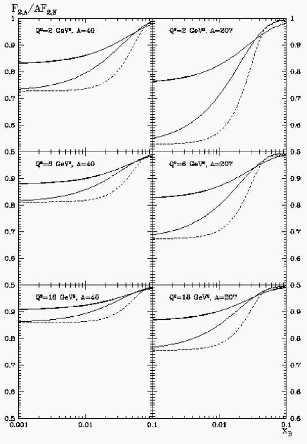
Figure 28: Nuclear shadowing for calcium and lead at different values of $Q^{2}$. The dashed curve is calculated in the standard approach (276), i.e. with coherence length $l_{c}=1/2m_{N}x_{Bj}$ and in double scattering approximation. The thin solid curve corresponds to the double scattering approximation with the free Green function, (200), and the thick solid curve shows the full calculation, (203).

The next step is to do the full calculation and to study the importance of the higher order rescattering terms in nuclear shadowing. The results are shown by the thick solid curves. Higher order scattering brings another substantial deviation (especially for lead) from the standard approach. At very low $x_{Bj}$ the curves saturate at the level given by (189). Note that the NM collaboration [162] was indeed unable to fit the $A$ dependence of the shadowing ratio at low $x_{Bj}$ with an ansatz linear in the nuclear density, indicating the importance of higher order rescattering terms.

However, calculations with (197) turn out to be numerically quite involved, if one wants to use a realistic parametrization of the DCS and a realistic nuclear density. The approximations introduced in this section significantly simplify the calculations, because one can find an analytic expression for the Green function $W$. We are forced to apply simplifying approximations also in our further calculations, but will use an effective $C$ in the dipole cross section in order to account for the correlation between the energy and $\rho$ dependence, as will be described in section 3.7. Then one can still make use of the solution (203) of the Schrödinger equation. This approach can be generalized to include also higher Fock components of the photon [13].

3.3 Derivation of the formula for nuclear shadowing in DIS

Before we start with the derivation, we briefly sketch the idea of the calculation. The applied approximations are summarized at the end of this subsection. For a nuclear target, the total cross section may be written in eikonal form (189), if the transverse separation $\rho$ is frozen, i.e. at very small $x_{Bj}$. The eikonal formula can be obtained in exactly the same way as by Glauber [7] in nonrelativistic quantum mechanics, because of the nonrelativistic structure of the light-cone Hamiltonian. In the eikonal approximation, one splits a fast oscillating phase factor from the wavefunction $\varphi(\vec{r})=e^{ikz}\tilde{\varphi}(\vec{r})$ and obtains for the slowly varying part $\tilde{\varphi}$ an equation of the form

$${\rm i}\frac{\partial}{\partial z}\tilde{\varphi}=\left(-\frac{\Delta_{\perp}}{const.}+V\right)\tilde{\varphi}.$$ (207)

In the target rest frame, the interaction is given by a color-static potential $V$. However, anticipating that all dependence of the interaction will be absorbed into the dipole cross section $\sigma_{q\bar{q}}(\rho)$, we use an abelian potential. Strictly speaking, this is justified only in the case of an electron-positron pair propagating in a condensed medium, but since the influence of the potential will be expressed in terms of scattering amplitudes and because our final result reproduces well known approximations in limiting cases, we believe, that the results holds also for the case of a nonabelian potential.

The Laplacian acts only on the transverse coordinates and is omitted in the eikonal approximation. Then, (207) is easily integrated. The multiple scattering series is summed like in Glauber theory [7]. This is possible, because the typical distance between two nucleons inside a nucleus is roughly $2$ fm, while the gluon correlation length is much smaller, presumably $\sim 0.3$ fm. After averaging over the medium, one obtains the eikonal expression (189).

The idea is now to keep this Laplacian, because it describes the transverse motion of the particles in the pair. Taking into account this motion, one can correctly describe the effective mass of the fluctuation in a coordinate space representation. The phase shift function has then to be replaced by the Green function for (207). We write this Green function as a path integral and averaging over all scattering centers yields an effective Green function $W$ which fulfills the two dimensional Schrödinger equation (197) with the optical potential $V_{opt}=-{\rm i}\sigma_{q\bar{q}}\left(\rho\right)\rho_{A}\left(b,z\right)/2$.

In order to derive explicit expressions for the terms in (192), we start from the general expression for the cross section for production of a $q\bar{q}$-pair,

$$d\sigma^{\gamma^{*}A} = Z_{f}^{2}\alpha_{em}\,\left|M_{fi}\right|^{2}\,\delta\left(\nu-p_{q}^{0}-p_{\bar{q}}^{0}\right)\frac{d^{3}p_{q}\,d^{3}p_{\bar{q}}}{\left(2\pi\right)^{4}\nu\,2p_{q}^{0}\,2p_{\bar{q}}^{0}}$$ (208)

$$= Z_{f}^{2}\alpha_{em}\,\left|M_{fi}\right|^{2}\,\frac{d^{2}p_{\perp,q}\,d^{2}p_{\perp,\bar{q}}\,d\lambda}{\left(2\pi\right)^{4}4\nu^{2}\,\lambda\left(1-\lambda\right)}$$ (209)

where $Z_{f}^{2}$ is the flavor charge, and $\alpha_{em}=1/137$. Note that we prefer to call the longitudinal momentum fraction of the quark by $\lambda$, because $\alpha$ is already used to denote many other quantities. The matrix element is given by

$$M_{fi}=\int d^{3}r\,\Psi_{q}^{\dagger}\left(\vec{r}\right)\,\vec{\bf\alpha}\cdot\vec{\epsilon}\;\Psi_{\bar{q}}\left(\vec{r}\right)e^{{\rm i}kz}.$$ (210)

The $z$-axis is chosen in direction of the propagation of the photon. The photon’s momentum is denoted by $k$ and it’s energy by $\nu$, $p_{q}$ is the momentum of the quark and $p_{\bar{q}}$ the momentum of the antiquark. In (209) we have introduced the energy fraction $\lambda=p_{q}^{0}/\nu$. In the ultrarelativistic case which is considered, pair production takes place predominantly in forward direction and therefore we distinguish between the longitudinal direction ($z$-direction) and the transverse directions. The longitudinal momenta are large compared to the flavor masses, $p_{z}\gg m_{f}$, and to the perpendicular momenta, $\left|\vec{p}_{\perp}\right|^{2}\sim m_{f}^{2}$. In our approximation, terms of order $m_{f}/p_{z}$ are kept only in exponentials and neglected otherwise. All higher order terms are omitted.

Note, that the pair is created electromagnetically in a color singlet state, therefore the factor $Z_{f}\alpha_{em}$ appears in (208), but the quarks interact with the nucleons as described by a phenomenological, scalar potential $\phi\left(\vec{r}\right)$. The particles in the pair move in a potential $U\left(\vec{r}\right)$ that is a superposition of the potentials of all nucleons,

$$U\left(\vec{r}\right)=\sum\limits_{j=1}^{A}\phi\left(\vec{r}-\vec{r}_{j}\right).$$ (211)

The vector $\vec{r}_{j}$ runs over all positions of the nucleons.

The wavefunction of the quark fulfills the Dirac equations and is an eigenstate with positive energy, while the antiquark is represented by an eigenstate with negative energy,

$$\left(p_{q}^{0}-U\left(\vec{r}\right)-m_{f}{\bf\beta}+{\rm i}\vec{\bf\alpha}\cdot\nabla\right)\Psi_{q}\left(\vec{r}\right) = 0,$$ (212)

$$\left(-p_{\bar{q}}^{0}-U\left(\vec{r}\right)-m_{f}{\bf\beta}+{\rm i}\vec{\bf\alpha}\cdot\nabla\right)\Psi_{\bar{q}}\left(\vec{r}\right) = 0.$$ (213)

No interaction between the quark and the antiquark is taken into account and therefore, the two equations decouple. The wavefunction of the quark $\Psi_{q}\left(\vec{r}\right)$ contains an outgoing plane wave and an outgoing spherical wave in it’s asymptotic form, while the wavefunction of the antiquark contains an incoming spherical wave and an incoming plane wave. These equations are transformed into second order equations by applying the operator $\left(p_{q}^{0}-U\left(\vec{r}\right)+m_{f}{\bf\beta}-{\rm i}\vec{\bf\alpha}\cdot\nabla\right)$ on the first equation, and the corresponding operator on the second equation, as described in [164]. When the term quadratic in the potential is omitted, one obtains

$$\left(\Delta+\left|\vec{p}_{q}\right|^{2}-2p_{q}^{0}U\left(\vec{r}\right)+{\rm i}\vec{\bf\alpha}\cdot\left(\nabla U\left(\vec{r}\right)\right)\right)\Psi_{q}\left(\vec{r}\right) = 0,$$ (214)

$$\left(\Delta+\left|\vec{p}_{\bar{q}}\right|^{2}+2p_{\bar{q}}^{0}U\left(\vec{r}\right)+{\rm i}\vec{\bf\alpha}\cdot\left(\nabla U\left(\vec{r}\right)\right)\right)\Psi_{\bar{q}}\left(\vec{r}\right) = 0.$$ (215)

The solutions may approximately be written as Furry [165, 166] type wavefunctions,

$$\Psi_{q}\left(\vec{r}\right) = e^{{\rm i}\vec{p}_{q}\cdot\vec{r}}\left(1-\frac{{\rm i}\vec{\bf\alpha}}{2p_{q}^{0}}\cdot\nabla\right)\,F_{q}\left(\vec{r}\right)\,u\left(p_{q},\lambda_{q}\right),$$ (216)

$$\Psi_{\bar{q}}\left(\vec{r}\right) = e^{-{\rm i}\vec{p}_{q}\cdot\vec{r}}\left(1+\frac{{\rm i}\vec{\bf\alpha}}{2p_{\bar{q}}^{0}}\cdot\nabla\right)\,F_{\bar{q}}\left(\vec{r}\right)\,v\left(p_{\bar{q}},\lambda_{\bar{q}}\right).$$ (217)

Here, $u\left(p_{q},\lambda_{q}\right)$ is the free spinor with positive energy and polarization $\lambda_{q}$ which fulfills the equation $\left(p_{q}\!\!\!\!\!/-m_{f}\right)u\left(p_{q},\lambda_{q}\right)=0$ and similarly $\left(p_{\bar{q}}\!\!\!\!\!/+m_{f}\right)v\left(p_{q},\lambda_{q}\right)=0$. In Dirac representation the spinors read

$$u\left(p_{q},\lambda_{q}\right)=\sqrt{p^{0}_{q}+m_{f}}\left(\begin{array}[]{c}\displaystyle{\chi_{q}}\\ \displaystyle{\frac{\vec{\sigma}\cdot\vec{p}_{q}}{p^{0}_{q}+m_{f}}\;\chi_{q}}\end{array}\right)\;\;,\;\;v\left(p_{q},\lambda_{q}\right)=\sqrt{p^{0}_{\bar{q}}+m_{f}}\left(\begin{array}[]{c}\displaystyle{\frac{\vec{\sigma}\cdot\vec{p}_{\bar{q}}}{p^{0}_{\bar{q}}+m_{f}}\;\chi_{\bar{q}}}\\ \displaystyle{\chi_{\bar{q}}}\end{array}\right).$$ (218)

The three Pauli spin matrices are denoted by $\vec{\sigma}$ and the Pauli spin state referred to the rest frame of the particle is $\chi_{q}$, or $\chi_{\bar{q}}$ respectivly. This means explicitly $\vec{s}\cdot\vec{\sigma}\,\chi_{q}=\lambda_{q}\chi_{q}$ and $\vec{s}\cdot\vec{\sigma}\,\chi_{\bar{q}}=-\lambda_{\bar{q}}\chi_{\bar{q}}$ with a spin vector $\vec{s}$ normalized to unity and $\lambda_{q},\lambda_{\bar{q}}=\pm 1$. The functions $F_{q}$ and $F_{\bar{q}}$ have no spinor structure any more. They contain all dependence of the potential and have to be calculated for a given $U\left(\vec{r}\right)$. They fulfill the equations [164]

$$\left(\Delta+2{\rm i}\vec{p}_{q}\cdot\nabla-2p_{q}^{0}U\left(\vec{r}\right)\right)F_{q}\left(\vec{r}\right) = 0,$$ (219)

$$\left(\Delta-2{\rm i}\vec{p}_{\bar{q}}\cdot\nabla+2p_{\bar{q}}^{0}U\left(\vec{r}\right)\right)q_{\bar{f}}\left(\vec{r}\right) = 0,$$ (220)

with boundary conditions $F\rightarrow 1$ for the quark and for the antiquark as $z\rightarrow\infty$. Note, that it is essential to take the correction proportional to $\vec{\alpha}$ in (216) and (217) into account, although these terms seem to be suppressed by a factor of $1/p^{0}$. It turns out, that when one calculates the matrix element of the current operator, $\left(\vec{\alpha}\cdot\vec{\epsilon}\,\right)_{fi}$, between free spinors, the large part cancels and one is left with a contribution of the same order as produced by the correction term. Thus, the terms proportional to $\vec{\alpha}$ may not be neglected in the matrix element, although they give only small corrections to the wave functions.

In order to remove the dependence on the transverse momenta from the phase factors in eq. (216) and (217), we rewrite the solutions in the form

$$\Psi_{q}\left(\vec{r}\right) = e^{{\rm i}\left|\vec{p}_{q}\,\right|z}\left(1-\frac{{\rm i}\vec{\bf\alpha}}{2p_{q}^{0}}\cdot\nabla-\frac{\vec{\bf\alpha}_{\perp}}{2p_{q}^{0}}\cdot\vec{p}_{\perp,q}+\frac{{\bf\alpha}_{z}}{2p_{q}^{0}}\left(\left|\vec{p}_{q}\,\right|-p_{z,q}\right)\right)\,\psi_{q}\left(\vec{r}\right)\,u\left(p_{q},\lambda_{q}\right),$$

$$\Psi_{\bar{q}}\left(\vec{r}\right) = e^{-{\rm i}\left|\vec{p}_{\bar{q}}\,\right|z}\left(1+\frac{{\rm i}\vec{\bf\alpha}}{2p_{\bar{q}}^{0}}\cdot\nabla-\frac{\vec{\bf\alpha}_{\perp}}{2p_{\bar{q}}^{0}}\cdot\vec{p}_{\perp,\bar{q}}+\frac{{\bf\alpha}_{z}}{2p_{q}^{0}}\left(\left|\vec{p}_{\bar{q}}\,\right|-p_{z,\bar{q}}\right)\right)\,\psi_{\bar{q}}\left(\vec{r}\right)\,v\left(p_{\bar{q}},\lambda_{\bar{q}}\right),$$

with

$$\psi_{q}\left(\vec{r}\right) = e^{{\rm i}\vec{p}_{\perp,q}\cdot\vec{r}_{\perp}}e^{-{\rm i}\left(\left|\vec{p}_{q}\,\right|-p_{z,q}\right)z}F_{q}\left(\vec{r}\right),$$ (223)

$$\psi_{\bar{q}}\left(\vec{r}\right) = e^{-{\rm i}\vec{p}_{\perp,\bar{q}}\cdot\vec{r}_{\perp}}e^{{\rm i}\left(\left|\vec{p}_{\bar{q}}\,\right|-p_{z,\bar{q}}\right)z}F_{\bar{q}}\left(\vec{r}\right),$$ (224)

and $\left|\vec{p}\,\right|=\sqrt{p_{0}^{2}-m_{f}^{2}}$ for the quark and the antiquark respectively. In the following, we neglect the terms with $\alpha_{z}$ in eq. (3.3) and (3.3), because they are of order $O\left(1/p^{0}_{q}p^{0}_{\bar{q}}\right)$. The functions $\psi_{q}\left(\vec{r}\right)$ and $\psi_{\bar{q}}\left(\vec{r}\right)$ will play the role of effective wave functions for the quarks.

The phase factors combine in the matrix element (210) to the minimal longitudinal momentum transfer,

$$q_{L}^{min}=k-\left|\vec{p}_{q}\,\right|-\left|\vec{p}_{\bar{q}}\,\right|\approx\frac{Q^{2}}{2\nu}+\frac{m_{f}^{2}}{2p_{0,q}}+\frac{m_{f}^{2}}{2p_{0,\bar{q}}},$$ (225)

and one obtains

$$M_{fi}\;=\;\int d^{3}re^{{\rm i}q_{L}^{min}z}$$ (226)

$$\times {\left[u^{\dagger}\left(p_{q},\lambda_{q}\right)\left(\,\vec{\bf\alpha}\cdot\vec{\epsilon}\;+\vec{\bf\alpha}\cdot\frac{{\rm i}\nabla\left(\vec{r}_{q}\right)-\vec{p}_{\perp,q}}{2p_{q}^{0}}\,\vec{\bf\alpha}\cdot\vec{\epsilon}\;+\vec{\bf\alpha}\cdot\vec{\epsilon}\,\vec{\bf\alpha}\cdot\frac{{\rm i}\nabla\left(\vec{r}_{\bar{q}}\right)-\vec{p}_{\perp,\bar{q}}}{2p_{\bar{q}}^{0}}\right)v\left(p_{\bar{q}},\lambda_{\bar{q}}\right)\right]}$$

$$\times \psi_{q}^{*}\left(\vec{r}_{{q}}\right)\psi_{\bar{q}}\left(\vec{r}_{\bar{q}}\right)\Big{|}_{\vec{r}=\vec{r}_{{q}}=\vec{r}_{\bar{q}}}.$$

Here, the coherence length, $l_{c}^{max}=1/q_{L}^{min}$, enters as an oscillating phase factor. However, $l_{c}^{max}$ does not depend on the transverse momenta. Their influence on the cross section is encoded in the rest of the wavefunctions, (3.3) and (3.3). The operator $\nabla\left(\vec{r}_{q}\right)$ acts only on the variable $\vec{r}_{q}$ and the operator $\nabla\left(\vec{r}_{\bar{q}}\right)$ only on $\vec{r}_{\bar{q}}$. After the derivatives have been performed, the whole integrand has to be evaluated at $\vec{r}=\vec{r}_{{q}}=\vec{r}_{\bar{q}}$.

With the representation (218) one obtains after some algebra within the demanded accuracy

$$M_{fi}\;=\;\int_{-\infty}^{\infty}dze^{{\rm i}q_{L}^{min}z}\int d^{2}r_{\perp}\frac{1}{\sqrt{\lambda\left(1-\lambda\right)}}$$ (227)

$$\times \chi_{q}^{\dagger}\displaystyle{\Bigg{\{}}m_{f}\vec{\sigma}\cdot\vec{\epsilon}_{T}+{\rm i}\left(1-\lambda\right)\vec{\sigma}\cdot\vec{e}_{z}\vec{\epsilon}_{T}\cdot\nabla\left(\vec{r}_{\perp,\bar{q}}\right)+{\rm i}\lambda\vec{\sigma}\cdot\vec{e}_{z}\vec{\epsilon}_{T}\cdot\nabla\left(\vec{r}_{\perp,{q}}\right)$$

$$+\left(1-\lambda\right)\left(\vec{e}_{z}\times\vec{\epsilon}_{T}\right)\cdot\nabla\left(\vec{r}_{\perp,{\bar{q}}}\right)-\lambda\left(\vec{e}_{z}\times\vec{\epsilon}_{T}\right)\cdot\nabla\left(\vec{r}_{\perp,{q}}\right)$$

$$+\;2\,Q\,\lambda\left(1-\lambda\right)\Bigg{\}}\chi_{\bar{q}}$$

$$\times \psi_{q}^{*}\left(\vec{r}_{\perp,{q}},z\right)\psi_{\bar{q}}\left(\vec{r}_{\perp,\bar{q}},z\right)\Big{|}_{\vec{r}_{\perp,{q}}=\vec{r}_{\perp,\bar{q}}}.$$

Some details of the calculation can be found in [167]. The unit vector in $z$-direction is denoted by $\vec{e}_{z}$. The polarization vector $\vec{\epsilon}_{T}$ corresponds to transverse states of the $\gamma^{*}$, while the last term in the curly brackets is due to longitudinal polarization. There are two remarkable aspect concerning this last equation. First, it does not contain any derivative with respect to $z$ any more, because of the transverse nature of the polarization vector $\vec{\epsilon}_{T}$ and of $\vec{e}_{z}\times\vec{\epsilon}_{T}$. Second, all dependence on the transverse momenta in the spinor part has canceled.

From (219) and (220) and from the definition of $\psi$, (223) and (224), an equation for $\psi$ is obtained. Assuming that these functions are only slowly varying with $z$, we omit the longitudinal part of the Laplacian and get

$${\rm i}\frac{\partial}{\partial z}\psi_{q}\left(\vec{r}_{\perp},z\right) = \left(-\frac{\Delta_{\perp}}{2p_{{q}}^{0}}+U\left(\vec{r}_{\perp},z\right)\right)\psi_{q}\left(\vec{r}_{\perp},z\right),$$ (228)

$${\rm i}\frac{\partial}{\partial z}\psi_{\bar{q}}\left(\vec{r}_{\perp},z\right) = \left(\frac{\Delta_{\perp}}{2p_{\bar{q}}^{0}}+U\left(\vec{r}_{\perp},z\right)\right)\psi_{\bar{q}}\left(\vec{r}_{\perp},z\right).$$ (229)

Our ansatz yields two dimensional Schrödinger equations, where the $z$-coordinate plays the role of time and the mass is given by the energy. The Laplacian $\Delta_{\perp}$ acts on the transverse coordinates only. The functions $\psi_{q}\left(\vec{r}_{\perp},z\right)$ and $\psi_{\bar{q}}\left(\vec{r}_{\perp},z\right)$ become two dimensional plane waves for $z\rightarrow\infty$, up to a phase factor that cancels in the square of the matrix element. It should be mentioned that the kinetic energy for the antiquark has a negative sign. This results from the fact that solutions of the Dirac equation with negative energy propagate backwards in time. The Laplacian in (228) and (229), account for the transverse motion of the pair in which we are especially interested. The functions $\psi_{\bar{q}}\left(\vec{r}_{\perp},z\right)$ and $\psi_{q}\left(\vec{r}_{\perp},z\right)$ in the matrix element (227) may now be expressed in terms of the Green functions for (228) and (229) and their asymptotic behavior,

$$\psi_{q}\left(\vec{r}_{\perp,2},z_{2}\right) = \int d^{2}r_{\perp,1}\,G_{q}\left(\vec{r}_{\perp,2},z_{2}\,|\,\vec{r}_{\perp,1},z_{\infty}\right)e^{{\rm i}\vec{p}_{\perp,q}\cdot\vec{r}_{\perp,1}}e^{-{\rm i}\left(\left|\vec{p}_{q}\,\right|-p_{z,q}\right)z_{\infty}},$$ (230)

$$\psi_{\bar{q}}\left(\vec{r}_{\perp,2},z_{2}\right) = \int d^{2}r_{\perp,1}\,G_{\bar{q}}\left(\vec{r}_{\perp,2},z_{2}\,|\,\vec{r}_{\perp,1},z_{\infty}\right)e^{-{\rm i}\vec{p}_{\perp,\bar{q}}\cdot\vec{r}_{\perp,1}}e^{{\rm i}\left(\left|\vec{p}_{\bar{q}}\,\right|-p_{z,\bar{q}}\right)z_{\infty}}.$$ (231)

Now one uses the expression for $d\sigma^{\gamma^{*}A}$, (208), and with the matrix element (227) and the last two relations, we obtain

$$d\sigma^{\gamma^{*}A} = Z_{f}^{2}\alpha_{em}\;\int_{-\infty}^{\infty}dz\int_{-\infty}^{\infty}dz^{\prime}e^{{\rm i}q_{L}^{min}\left(z-z^{\prime}\right)}\int d^{2}r_{\perp}\,d^{2}\tau_{q}\,d^{2}\tau_{\bar{q}}\,\int d^{2}r_{\perp}^{\,\prime}\,d^{2}\tau_{q}^{\prime}\,d^{2}\tau_{\bar{q}}^{\prime}\,$$ (232)

$$\;\;\;\times\;\;{\cal O}\left(\vec{r}_{\perp,{q}},\vec{r}_{\perp,\bar{q}}\right)G_{q}^{*}\left(\vec{r}_{\perp,{q}},z\,|\,\vec{\tau}_{q},z_{\infty}\right)\,G_{\bar{q}}\left(\vec{r}_{\perp,\bar{q}},z\,|\,\vec{\tau}_{\bar{q}},z_{\infty}\right)\Big{|}_{\vec{r}_{\perp}=\vec{r}_{\perp,{q}}=\vec{r}_{\perp,\bar{q}}}$$

$$\;\;\;\times\;\;{\cal O}^{*}\left(\vec{r}^{\,\prime}_{\perp,{q}},\vec{r}^{\,\prime}_{\perp,\bar{q}}\right)G_{q}\left(\vec{r}_{\perp,{q}}^{\,\prime},z^{\,\prime}\,|\,\vec{\tau}_{q}^{\,\prime},z_{\infty}\right)\,G_{\bar{q}}^{*}\left(\vec{r}_{\perp,\bar{q}}^{\,\prime},z^{\,\prime}\,|\,\vec{\tau}_{\bar{q}}^{\,\prime},z_{\infty}\right)\Big{|}_{\vec{r}_{\perp}^{\,\prime}=\vec{r}_{\perp,{q}}^{\,\prime}=\vec{r}^{\,\prime}_{\perp,\bar{q}}}$$

$$\;\;\;\times\;\;e^{{\rm i}\left(\vec{\tau}_{q}^{\,\prime}-\vec{\tau}_{q}\right)\cdot\vec{p}_{\perp,q}}\,e^{{\rm i}\left(\vec{\tau}_{\bar{q}}^{\,\prime}-\vec{\tau}_{\bar{q}}\right)\cdot\vec{p}_{\perp,\bar{q}}}$$

$$\;\;\;\times\;\;\frac{d^{2}p_{\perp,q}\,d^{2}p_{\perp,\bar{q}}\,d\lambda}{\left(2\pi\right)^{4}\,\lambda^{2}\left(1-\lambda\right)^{2}4\nu^{2}}.$$

For convenience the operator

$${\cal O}\left(\vec{r}_{\perp,{q}},\vec{r}_{\perp,\bar{q}}\right) = \chi_{q}^{\dagger}\displaystyle{\Bigg{\{}}m_{f}\vec{\sigma}\cdot\vec{\epsilon}_{T}+{\rm i}\left(1-\lambda\right)\vec{\sigma}\cdot\vec{e}_{z}\vec{\epsilon}_{T}\cdot\nabla\left(\vec{r}_{\perp,\bar{q}}\right)+{\rm i}\lambda\vec{\sigma}\cdot\vec{e}_{z}\vec{\epsilon}_{T}\cdot\nabla\left(\vec{r}_{\perp,{q}}\right)$$ (233)

$$+ \left(1-\lambda\right)\left(\vec{e}_{z}\times\vec{\epsilon}_{T}\right)\cdot\nabla\left(\vec{r}_{\perp,{\bar{q}}}\right)-\lambda\left(\vec{e}_{z}\times\vec{\epsilon}_{T}\right)\cdot\nabla\left(\vec{r}_{\perp,{q}}\right)$$

$$+ 2\,Q\,\lambda\left(1-\lambda\right)\vec{\sigma}\cdot\vec{e}_{z}\Bigg{\}}\chi_{\bar{q}}$$ (234)

is introduced. In order to obtain the total cross section, we integrate over $p_{\perp,q}$ and $p_{\perp,\bar{q}}$. The exponential factors give a $\delta$-function which makes it possible to perform the integrations over all the $\tau$s. Note, that ${\cal O}$ does not depend on $\tau$. The result is

$$\sigma_{tot}^{\gamma^{*}A} = Z_{f}^{2}\,\frac{\alpha_{em}}{\nu^{2}}\,2{\rm Re}\int\limits_{0}^{1}\frac{d\lambda}{\lambda^{2}\left(1-\lambda\right)^{2}}\;\int\limits_{-\infty}^{\infty}dz\int\limits_{z}^{\infty}dz^{\prime}e^{{\rm i}q_{min}\left(z-z^{\prime}\right)}\int d^{2}r_{\perp}\,\int d^{2}r_{\perp}^{\,\prime}$$ (235)

$$\;\;\;\times\;\;{\cal O}\left(\vec{r}_{\perp,{q}},\vec{r}_{\perp,\bar{q}}\right){\cal O}^{*}\left(\vec{r}^{\,\prime}_{\perp,{q}},\vec{r}^{\,\prime}_{\perp,\bar{q}}\right)$$

$$\;\;\;\times\;\;G_{q}\left(\vec{r}_{\perp,q}^{\,\prime},z^{\,\prime}\,|\vec{r}_{\perp,q},z\right)\,G_{\bar{q}}^{*}\left(\vec{r}_{\perp,\bar{q}}^{\,\prime},z^{\,\prime}\,|\vec{r}_{\perp,\bar{q}},z\right)\Big{|}_{\vec{r}_{\perp}=\vec{r}_{\perp,{q}}=\vec{r}_{\perp,\bar{q}}\,;\,\vec{r}_{\perp}^{\,\prime}=\vec{r}_{\perp,{q}}^{\,\prime}=\vec{r}^{\,\prime}_{\perp,\bar{q}}}.$$

Instead of four propagators one is left with only two, because of the convolution relation

$$G\left(\vec{r}_{\perp,2},z_{2}\,|\,\vec{r}_{\perp,1},z_{1}\right)=\int d^{2}r_{\perp}\;G\left(\vec{r}_{\perp,2},z_{2}\,|\,\vec{r}_{\perp},z\right)G\left(\vec{r}_{\perp},z\,|\,\vec{r}_{\perp,1},z_{1}\right).$$ (236)

In order to derive an expression that is convenient for numerical calculations, one makes use of the path-integral representations of the propagators in (235). They read

$$G\left(\vec{r}_{\perp}^{\,\prime},z^{\,\prime}\,|\vec{r}_{\perp},z\right)=\!\!\int{\cal D}\vec{\tau}\,\exp\left\{{\rm i}\int\limits^{z^{\,\prime}}_{z}d\xi\left(\pm\frac{p^{0}}{2}\dot{\vec{\tau}}^{\,2}-U\left(\vec{\tau},\xi\right)\right)\right\}$$

$$\approx \!\!\int{\cal D}\vec{\tau}\,\exp\left\{{\rm i}\!\int\limits^{z_{2}}_{z_{1}}\pm\frac{p^{0}}{2}\dot{\vec{\tau}}^{\,2}d\xi-{\rm i}\sum\limits_{j=1}^{A}\mbox{X}\left(\vec{\tau}\left(z_{j}\right)-\vec{r}_{j,\perp}\right)\Theta\left(z^{\,\prime}-z_{j}\right)\Theta\left(z_{j}-z\right)\right\},$$

where the upper sign corresponds to the quark and the lower to the antiquark. In this expression, $\vec{\tau}$ is a function of $\xi$. The derivative with respect to $\xi$ is denoted by $\dot{\vec{\tau}}$. Furthermore, the condition

$$G\left(\vec{r}_{\perp}^{\,\prime},z^{\,\prime}\,|\vec{r}_{\perp},z\right)\Big{|}_{z^{\,\prime}=z}=\delta^{(2)}\left(\vec{r}_{\perp}^{\,\prime}-\vec{r}_{\perp}\right)$$ (239)

has to be fulfilled together with $\vec{\tau}\left(z\right)=\vec{r}_{\perp}$ and $\vec{\tau}\left(z^{\,\prime}\right)=\vec{r}_{\perp}^{\,\prime}$. In (3.3), the phase shift function $\mbox{X}\left(\vec{\tau}-\vec{r}_{j,\perp}\right)$ is introduced. The step function $\Theta\left(z\right)$ is $0$ for $z<0$ and $1$ for $z>0$. As mentioned before, $U$ is the superposition of all potentials of the nucleons, see eq. (211). Let $\phi$ be the potential of a single nucleon in the target. The position of the nucleon with number $j$ is denoted by the transverse vector $\vec{r}_{j,\perp}$ and the longitudinal coordinate $z_{j}$. If the range of interaction is much smaller than the distance $z^{\,\prime}-{z}$, the potential is practically zero outside the domain of integration over $\xi$ and the phase shift function is given by

$$\mbox{X}\left(\vec{r}_{\perp}-\vec{r}_{j,\perp}\right)=\int_{-\infty}^{\infty}d\xi\,\phi\left(\vec{r}_{\perp}-\vec{r}_{j,\perp},\xi-z_{j}\right).$$ (240)

Note that $\vec{\tau}\left(\xi\right)$ was replaced by $\vec{\tau}\left(z_{j}\right)$. This means, only an average value of the transverse coordinate is used for calculating the phase shift for scattering on a single nucleon.

The two path integrals (3.3) for the quark ($+$) and the antiquark ($-$) sum over all possible trajectories of the two particles. In order to calculate the cross section for pair production in the nuclear medium, one has to average over all nucleons. One obtains with the path-integral (3.3)

$$\left<G_{q}\left(\vec{r}_{\perp,q}^{\,\prime},z^{\,\prime}\,|\vec{r}_{\perp,q},z\right)\,G_{\bar{q}}^{*}\left(\vec{r}_{\perp,\bar{q}}^{\,\prime},z^{\,\prime}\,|\vec{r}_{\perp,\bar{q}},z\right)\right>$$ (242)

$$= \left<\int{\cal D}\vec{\tau}_{q}\,\int{\cal D}\vec{\tau}_{\bar{q}}\,\exp\left\{{\rm i}\int\limits^{z^{\,\prime}}_{z}\left(\frac{p_{q}^{0}}{2}\dot{\vec{\tau}}_{q}^{\,2}+\frac{p^{0}_{\bar{q}}}{2}\dot{\vec{\tau}}_{\bar{q}}^{\,2}\right)d\xi\right.\right.$$

$$\left.\left.+{\rm i}\sum\limits_{j=1}^{A}\Theta\left(z^{\,\prime}-z_{j}\right)\Theta\left(z_{j}-z\right)\Bigl{(}\mbox{X}\left(\vec{\tau}_{\bar{q}}\left(z_{j}\right)-\vec{r}_{j,\perp}\right)-\mbox{X}\left(\vec{\tau}_{q}\left(z_{j}\right)-\vec{r}_{j,\perp}\right)\Bigr{)}\right\}\right>,$$

with boundary conditions $\vec{\tau}_{q}\left(z\right)=\vec{r}_{\perp,q}$, $\vec{\tau}_{q}\left(z^{\,\prime}\right)=\vec{r}_{\perp,q}^{\,\prime}$, $\vec{\tau}_{\bar{q}}\left(z\right)=\vec{r}_{\perp,\bar{q}}$ and $\vec{\tau}_{\bar{q}}\left(z^{\,\prime}\right)=\vec{r}_{\perp,\bar{q}}^{\,\prime}$. The averaging procedure is similar to the one described in [7]. All correlations between the nucleons are neglected and the average nuclear density ${\rho_{A}}$ is introduced, which is normalized to $A$, (LABEL:density). Then, the whole expression may be written as an exponential, if $A$ is large enough,

$$\left<\exp\left({\rm i}\sum\limits_{j=1}^{A}\Theta\left(z^{\,\prime}-z_{j}\right)\Theta\left(z_{j}-z\right)\Bigl{(}\mbox{X}\left(\vec{\tau}_{\bar{q}}\left(z_{j}\right)-\vec{r}_{j,\perp}\right)-\mbox{X}\left(\vec{\tau}_{q}\left(z_{j}\right)-\vec{r}_{j,\perp}\right)\Bigr{)}\right)\right>$$ (244)

$$= \Biggl{\{}1-\frac{1}{A}\int d^{2}s\int\limits^{z^{\,\prime}}_{z}d\xi^{\,\prime}{\rho_{A}}\left(\vec{s},\xi^{\,\prime}\right)$$

$$\times \Biggl{.}\left(1-\exp\Biggl{(}{\rm i}\Bigl{(}\,\mbox{X}\left(\vec{\tau}_{\bar{q}}\left(\xi^{\,\prime}\right)-\vec{s}\right)-\,\mbox{X}\left(\vec{\tau}_{q}\left(\xi^{\,\prime}\right)-\vec{s}\right)\Bigr{)}\Biggr{)}\right)\Biggr{\}}^{A}$$

$$\approx \exp\left\{-\int\limits^{z^{\,\prime}}_{z}d\xi^{\,\prime}{\rho_{A}}\left(b,\xi^{\,\prime}\right)\right.$$

$$\;\;\times\left.\;\;\int d^{2}s\left(1-\exp\Biggl{(}{\rm i}\Bigl{(}\,\mbox{X}\left(\vec{\tau}_{\bar{q}}\left(\xi^{\,\prime}\right)-\vec{s}\right)-\,\mbox{X}\left(\vec{\tau}_{q}\left(\xi^{\,\prime}\right)-\vec{s}\right)\Bigr{)}\Biggr{)}\right)\right\}.$$

When ${\rho_{A}}$ is varying fairly smoothly inside the nucleus, one can replace its dependence of $\vec{s}$, the transverse distance between the pair and the scattering nucleon, by the impact parameter $b$, eq. (LABEL:app). Since we have a short ranged interaction, it is reasonable to choose as impact parameter $\vec{b}=\left(\vec{r}_{\perp}-\vec{r}_{\perp}^{\,\prime}\right)/2$. This way one finds the forward scattering amplitude for a dipole scattering on a single nucleon, see eq. (LABEL:app). The corresponding cross section,

$$\sigma_{q\bar{q}}\left(\rho\right)=2{\rm Re}\int d^{2}s\left(1-\exp\Biggl{(}{\rm i}\Bigl{(}\mbox{X}\left(\vec{\rho}-\vec{s}\right)-\mbox{X}\left(\vec{s}\right)\Bigr{)}\Biggr{)}\right),$$ (245)

appears as imaginary potential in the propagator. At this point one notices that the forward scattering amplitude in the abelian model is predominantly real, while in a nonabelian theory it has to be imaginary. Nevertheless, we believe that the final result holds also for a nonabelian theory, because all dependence on the potential of the nucleons, $\phi\left(\vec{r}\right)$, is absorbed into $\sigma_{q\bar{q}}$, for which we will use a parametrization. One finally arrives at

$$\left<G_{q}\left(\vec{r}_{\perp,q}^{\,\prime},z^{\,\prime}\,|\vec{r}_{\perp,q},z\right)\,G_{\bar{q}}^{*}\left(\vec{r}_{\perp,\bar{q}}^{\,\prime},z^{\,\prime}\,|\vec{r}_{\perp,\bar{q}},z\right)\right>$$ (246)

$$= \!\!\!\int{\cal D}\vec{\tau}_{q}\int{\cal D}\vec{\tau}_{\bar{q}}\exp\left\{{\rm i}\int\limits^{z^{\,\prime}}_{z}d\xi\left(\frac{p_{q}^{0}}{2}\dot{\vec{\tau}}_{q}^{\,2}+\frac{p^{0}_{\bar{q}}}{2}\dot{\vec{\tau}}_{\bar{q}}^{\,2}+\frac{{\rm i}}{2}{\rho_{A}}\left(b,\xi\right)\sigma_{q\bar{q}}\left(\left|\vec{\tau}_{q}-\vec{\tau}_{\bar{q}}\right|\right)\right)\right\}.$$

It is convenient to introduce center of mass coordinates, $\vec{\tau}_{rel}=\vec{\tau}_{\bar{q}}-\vec{\tau}_{q}$ and $\vec{\tau}_{cm}=\left(1-\lambda\right)\vec{\tau}_{\bar{q}}+\lambda\vec{\tau}_{q}$, and to express the sum of the two kinetic energies as the sum of the kinetic energy of the relative motion and the center of mass kinetic energy,

$$\left<G_{q}\left(\vec{r}_{\perp,q}^{\,\prime},z^{\,\prime}\,|\vec{r}_{\perp,q},z\right)\,G_{\bar{q}}^{*}\left(\vec{r}_{\perp,\bar{q}}^{\,\prime},z^{\,\prime}\,|\vec{r}_{\perp,\bar{q}},z\right)\right>$$ (248)

$$= \int{\cal D}\vec{\tau}_{cm}\,\int{\cal D}\vec{\tau}_{rel}\,\exp\left\{{\rm i}\int\limits^{z^{\,\prime}}_{z}d\xi\left(\frac{\mu}{2}\dot{\vec{\tau}}_{rel}^{\,2}+\frac{\nu}{2}\dot{\vec{\tau}}_{cm}^{\,2}+\frac{{\rm i}}{2}{\rho_{A}}\left(b,\xi\right)\sigma_{q\bar{q}}\left(\tau_{rel}\right)\right)\right\}$$

$$= \frac{\nu}{2\pi{\rm i}\left(z^{\,\prime}-z\right)}\,\exp\left({\rm i}\frac{\nu}{2}\frac{\left(\lambda\left(\vec{r}_{\perp,q}^{\,\prime}-\vec{r}_{\perp,q}\right)+\left(1-\lambda\right)\left(\vec{r}_{\perp,\bar{q}}^{\,\prime}-\vec{r}_{\perp,\bar{q}}\right)\right)^{2}}{z^{\,\prime}-z}\right)$$

$$\;\;\;\times\;\;\int{\cal D}\vec{\tau}_{rel}\,\exp\left\{{\rm i}\int\limits^{z^{\,\prime}}_{z}d\xi\left(\frac{\mu}{2}\dot{\vec{\tau}}_{rel}^{\,2}+\frac{{\rm i}}{2}{\rho_{A}}\left(b,\xi\right)\sigma_{q\bar{q}}\left(\tau_{rel}\right)\right)\right\}.$$

We have introduced the reduced mass

$$\frac{1}{\mu}=\frac{1}{p_{q}^{0}}+\frac{1}{p_{\bar{q}}^{0}}=\frac{1}{\nu\lambda\left(1-\lambda\right)}.$$ (249)

Since the imaginary potential depends only on the relative coordinate, the center of mass propagates freely and what remains is the effective propagator

$$W\left(\vec{\rho}^{\,\prime},z^{\,\prime}\,|\,\vec{\rho},z\right)=\int{\cal D}\vec{\tau}_{rel}\,\exp\left\{{\rm i}\int\limits^{z^{\,\prime}}_{z}d\xi\left(\frac{\mu}{2}\dot{\vec{\tau}}_{rel}^{\,2}-V_{opt}\left(b,\tau_{rel},\xi\right)\right)\right\},$$ (250)

with $\vec{\rho}^{\,\prime}=\vec{r}_{\perp,\bar{q}}^{\,\prime}-\vec{r}_{\perp,q}^{\,\prime}$ and $\vec{\rho}=\vec{r}_{\perp,\bar{q}}-\vec{r}_{\perp,q}$ and the optical potential

$$V_{opt}\left(b,\rho,z\right)=-\frac{{\rm i}}{2}{\rho_{A}}\left(b,z\right)\sigma_{q\bar{q}}\left(\rho\right).$$ (251)

It fulfills the equation

$$\left[{\rm i}\frac{\partial}{\partial z^{\,\prime}}+\frac{\Delta_{\perp}\left(\rho^{\,\prime}\right)}{2\nu\lambda\left(1-\lambda\right)}-V_{opt}\left(b,\rho^{\,\prime},z^{\,\prime}\right)\right]W\left(\vec{\rho}^{\,\prime},z^{\,\prime}\,|\,\vec{\rho},z\right)={\rm i}\delta\left(z^{\,\prime}-z\right)\delta^{\left(2\right)}\left(\vec{\rho}^{\,\prime}-\vec{\rho}\right).$$ (252)

The propagator for the center of mass coordinate produces a $\delta$-function and thus, one obtains from (235) after averaging over the medium

$$\sigma_{tot}^{\gamma^{*}A} = \frac{Z_{f}^{2}\alpha_{em}}{4\nu^{2}}\,\int d^{2}b\;2{\rm Re}\int\limits_{0}^{1}\frac{d\lambda}{\lambda^{2}\left(1-\lambda\right)^{2}}\;\int\limits_{-\infty}^{\infty}dz\int\limits_{z}^{\infty}dz^{\prime}e^{{\rm i}q_{L}^{min}\left(z-z^{\prime}\right)}$$ (253)

$$\;\;\;\times\;\;{\cal O}_{q\bar{q}}\left(\vec{\rho}\right){\cal O}_{q\bar{q}}^{*}\left(\vec{\rho}^{\,\prime}\right)\;W\left(\vec{\rho}^{\,\prime},z^{\,\prime}\,|\,\vec{\rho},z\right)\Big{|}_{\vec{\rho}^{\,\prime}=\vec{\rho}=\vec{0}},$$

with

$${\cal O}_{q\bar{q}}\left(\vec{\rho}\right)={\cal O}_{q\bar{q}}^{T}\left(\vec{\rho}\right)+{\cal O}_{q\bar{q}}^{L}\left(\vec{\rho}\right),$$ (254)

where the transverse part of the operator is

$${\cal O}_{q\bar{q}}^{T}\left(\vec{\rho}\right)=\chi_{q}^{\dagger}\displaystyle{\Bigg{\{}}m_{f}\vec{\sigma}\cdot\vec{\epsilon}_{T}+{\rm i}\left(1-2\lambda\right)\vec{\sigma}\cdot\vec{e}_{z}\vec{\epsilon}_{T}\cdot\nabla\left(\vec{\rho}\right)+\left(\vec{e}_{z}\times\vec{\epsilon}_{T}\right)\cdot\nabla\left(\vec{\rho}\right)\Bigg{\}}\chi_{\bar{q}}$$ (255)

and the longitudinal part

$${\cal O}_{q\bar{q}}^{L}\left(\vec{\rho}\right)=\chi_{q}^{\dagger}2\,Q\,\lambda\left(1-\lambda\right)\vec{\sigma}\cdot\vec{e}_{z}\chi_{\bar{q}}=2\,Q\,\lambda\left(1-\lambda\right)\delta_{\lambda_{q},\lambda_{\bar{q}}}.$$ (256)

These operators are already known from the definition of the LC wavefunctions in section 2.3, see (70,71). Equation (253) is the central result of this section. It is the total cross section for production of a $q\bar{q}$-pair from a virtual photon scattering on a nucleus. We have not summed over the spins of the quark and the antiquark and not averaged over the polarizations of the photon. We have not summed over the different flavors, either. The expression for the operator ${\cal O}$, (254), depends on the spin vector of the quark and the antiquark. The directions of these vectors may be fixed arbitrarily.

In order to represent the result in the form (192), $W$ and it’s complex conjugate is rewritten in an expansion. The results can be combined in the following way:

$$W\left(\vec{\rho}^{\,\prime},z^{\,\prime}\,|\,\vec{\rho},z\right) = W_{0}\left(\vec{\rho}^{\,\prime},z^{\,\prime}\,|\,\vec{\rho},z\right)$$ (257)

$$+ {\rm i}\int\limits_{z}^{z^{\,\prime}}dz_{1}\int d^{2}\rho_{1}W_{0}\left(\vec{\rho}^{\,\prime},z^{\,\prime}\,|\,\vec{\rho}_{1},z_{1}\right)\,V_{opt}\left(b,\rho_{1},z_{1}\right)\,W_{0}\left(\vec{\rho}_{1},z_{1}\,|\,\vec{\rho},z\right)$$

$$- \int\limits_{z}^{z^{\,\prime}}dz_{1}\int d^{2}\rho_{1}\int\limits_{z}^{z_{1}}dz_{2}\int d^{2}\rho_{2}W_{0}\left(\vec{\rho}^{\,\prime},z^{\,\prime}\,|\,\vec{\rho}_{1},z_{1}\right)\,V_{opt}^{*}\left(b,\rho_{1},z_{1}\right)\,$$

$$\;\;\times\;\;W\left(\vec{\rho}_{1},z_{1}\,|\,\vec{\rho}_{2},z_{2}\right)V_{opt}\left(b,\rho_{2},z_{2}\right)\,W_{0}\left(\vec{\rho}_{2},z_{2}\,|\,\vec{\rho},z\right).$$

Here, $W_{0}$ is the propagator corresponding to (250), when the potential is absent. The first term gives a divergent contribution, which is the wave-function renormalization for the photon. The second term leads to the first contribution in (192). The operators ${\cal O}_{q\bar{q}}^{T,L}$ applied to the free propagator $W_{0}$ give the light-cone wave functions $\Psi^{T,L}_{q\bar{q}}\left(\rho,\lambda\right)$, up to a constant overall factor. The third term in the above expansion is the interference term. Since this term contains the full propagator, there are no higher terms in this expansion.

As an example for further calculation, consider the integral

$$\cal{I} = -\int\limits_{-\infty}^{\infty}dz\int\limits_{z}^{\infty}dz^{\prime}{\rm e}^{{\rm i}q_{L}^{min}\left(z-z^{\prime}\right)}\int\limits_{z}^{z^{\,\prime}}dz_{1}\int d^{2}\rho_{1}\int\limits_{z}^{z_{1}}dz_{2}\int d^{2}\rho_{2}$$ (258)

$$\;\;\times\;\;V_{opt}^{*}\left(b,\rho_{1},z_{1}\right)\,V_{opt}\left(b,\rho_{2},z_{2}\right)$$

$$\;\;\times\;\;W_{0}\left(\vec{\rho}^{\,\prime},z^{\,\prime}\,|\,\vec{\rho}_{1},z_{1}\right)\,W\left(\vec{\rho}_{1},z_{1}\,|\,\vec{\rho}_{2},z_{2}\right)W_{0}\left(\vec{\rho}_{2},z_{2}\,|\,\vec{\rho},z\right),$$

which is needed to calculate the interference part

$$\sigma_{tot}^{int}=\frac{Z_{f}^{2}\alpha_{em}}{4\nu^{2}}\,\int d^{2}b\;2{\rm Re}\int\limits_{0}^{1}\frac{d\lambda}{\lambda^{2}\left(1-\lambda\right)^{2}}{\cal O}\left(\vec{\rho}\right){\cal O}^{*}\left(\vec{\rho}^{\,\prime}\right)\;{\cal I}\,\Big{|}_{\vec{\rho}^{\,\prime}=\vec{\rho}=\vec{0}}.$$ (259)

With the new variable $\varepsilon^{2}=\lambda\left(1-\lambda\right)\,Q^{2}+m_{f}^{2}$, which is also defined in 47, one finds

$$q_{L}^{min}=\frac{\varepsilon^{2}}{2\nu\lambda\left(1-\lambda\right)},$$ (260)

and because of the relation

$$\left[{\rm i}\frac{\partial}{\partial z^{\,\prime}}+\frac{\Delta_{\perp}\left(\rho^{\,\prime}\right)-\varepsilon^{2}}{2\nu\lambda\left(1-\lambda\right)}\right]\left(W_{0}\left(\vec{\rho}^{\,\prime},z^{\,\prime}\,|\,\vec{\rho},z\right)e^{-{\rm i}q_{L}^{min}\left(z^{\,\prime}-z\right)}\right)={\rm i}\delta\left(z^{\,\prime}-z\right)\delta^{\left(2\right)}\left(\vec{\rho}^{\,\prime}-\vec{\rho}\right),$$ (261)

one can write the propagator in the form

$$W_{0}\left(\vec{\rho}^{\,\prime},z^{\,\prime}\,|\,\vec{\rho},z\right)e^{-{\rm i}q_{L}^{min}\left(z^{\,\prime}-z\right)}=\int\frac{d^{2}l_{\perp}}{\left(2\pi\right)^{2}}\int\limits_{-\infty}^{\infty}\frac{d\omega}{2\pi}\;\frac{\exp\left\{-{\rm i}\omega\left(z^{\,\prime}-z\right)+{\rm i}\vec{l}_{\perp}\cdot\left(\vec{\rho}^{\,\prime}-\vec{\rho}\right)\right\}}{{\omega-\displaystyle{\frac{\vec{l}_{\perp}^{2}+\varepsilon^{2}}{2\nu\lambda\left(1-\lambda\right)}}+{\rm i}0_{+}}}.$$ (262)

The $0_{+}$-prescription for the pole in the complex $\omega$-plane ensures that $W_{0}\left(\vec{\rho}^{\,\prime},z^{\,\prime}\,|\,\vec{\rho},z\right)=0$ for $z>z^{\,\prime}$. Putting (262) into (258) yields after a short calculation

$$\cal{I} = -\frac{4\nu^{2}\lambda^{2}\left(1-\lambda\right)^{2}}{\left(2\pi\right)^{2}}\int\limits_{-\infty}^{\infty}dz_{1}\int\limits_{-\infty}^{z_{1}}dz_{2}e^{{\rm i}q_{L}^{min}\left(z_{2}-z_{1}\right)}\int d^{2}\rho_{1}\int d^{2}\rho_{2}$$ (263)

$$\;\;\times\;\;V_{opt}^{*}\left(b,\rho_{1},z_{1}\right)\,V_{opt}\left(b,\rho_{2},z_{2}\right)$$

$$\;\;\times\;\;{\rm K}_{0}\left(\varepsilon\left|\vec{\rho}^{\,\prime}-\vec{\rho}_{1}\right|\right)W\left(\vec{\rho}_{1},z_{1}\,|\,\vec{\rho}_{2},z_{2}\right){\rm K}_{0}\left(\varepsilon\left|\vec{\rho}_{2}-\vec{\rho}\right|\right).$$

K₀ is the MacDonald function of zeroth order. We have used the relation

$${\rm K}_{0}\left(\varepsilon\rho\right)=\frac{1}{2\pi}\int d^{2}l_{\perp}\frac{{\rm e}^{{\rm i}\vec{l}_{\perp}\cdot\vec{\rho}}}{l_{\perp}^{2}+\varepsilon^{2}}.$$ (264)

The next step is to insert (263) into (259) and to calculate the contribution from the second term in the expansion (257) in a similar way. One obtains for the total cross section

$$\sigma_{tot}^{\gamma^{*}\,A} = A\,Z_{f}^{2}\,\frac{\alpha_{em}}{\left(2\pi\right)^{2}}\int\limits_{0}^{1}d\lambda\int d^{2}\rho_{1}\,\sigma_{q\bar{q}}\left(\rho_{1}\right)\,\left|{\cal O}_{q\bar{q}}\left(\vec{\rho}\right){\rm K}_{0}\left(\varepsilon\left|\vec{\rho}-\vec{\rho}_{1}\right|\right)\Big{|}_{\vec{\rho}=\vec{0}}\right|^{2}$$ (265)

$$- Z_{f}^{2}\,\frac{\alpha_{em}}{\left(2\pi\right)^{2}}\,2{\rm Re}\int d^{2}b\int\limits_{-\infty}^{\infty}dz_{1}\int\limits_{z_{1}}^{\infty}dz_{2}\int\limits_{0}^{1}d\lambda\int d^{2}\rho_{1}\int d^{2}\rho_{2}\,e^{-{\rm i}q_{L}^{min}\left(z_{2}-z_{1}\right)}$$

$$\;\;\times\;\;V_{opt}^{*}\left(b,\rho_{1},z_{1}\right)\,V_{opt}\left(b,\rho_{2},z_{2}\right)\left({\cal O}_{q\bar{q}}^{*}\left(\vec{\rho}^{\,\prime}\right){\rm K}_{0}\left(\varepsilon\left|\vec{\rho}^{\,\prime}-\vec{\rho}_{1}\right|\right)\Big{|}_{\vec{\rho}^{\,\prime}=\vec{0}}\right)$$

$$\;\;\times\;\;W\left(\vec{\rho}_{2},z_{2}\,|\,\vec{\rho}_{1},z_{1}\right)\,\left({\cal O}_{q\bar{q}}\left(\vec{\rho}\right){\rm K}_{0}\left(\varepsilon\left|\vec{\rho}-\vec{\rho}_{2}\right|\right)\Big{|}_{\vec{\rho}=\vec{0}}\right).$$

With help of the relation

$$\nabla\left(\vec{\rho}\right){\rm K}_{0}\left(\varepsilon\rho\right)=-\varepsilon\frac{\vec{\rho}}{\rho}{\rm K}_{1}\left(\varepsilon\rho\right)$$ (266)

one finds the light-cone wave functions

$$\Psi^{T}_{q\bar{q}}\left(\alpha,\vec{\rho}\right) = Z_{f}\,\frac{\sqrt{\alpha_{em}}}{2\pi}{\cal O}_{q\bar{q}}^{T}\left(\vec{\rho}\right){\rm K}_{0}\left(\varepsilon\rho\right)$$ (268)

$$= Z_{f}\,\frac{\sqrt{\alpha_{em}}}{2\pi}\Bigg{\{}m\,{\rm K}_{0}\left(\varepsilon\rho\right)\,\delta_{\lambda_{q},\lambda_{\bar{q}}}\,\delta_{\lambda_{q},\lambda_{\gamma}}$$

$$+\Bigl{(}{\rm i}\lambda_{q}\left(2\lambda-1\right)\vec{\epsilon}_{T}\cdot\vec{e}_{\rho}+\left(\vec{\epsilon}_{T}\times\vec{e}_{z}\right)\cdot\vec{e}_{\rho}\Bigr{)}\varepsilon{\rm K}_{1}\left(\varepsilon\rho\right)\delta_{\lambda_{q},-\lambda_{\bar{q}}}\Bigg{\}}$$

and

$$\Psi^{L}_{q\bar{q}}\left(\alpha,\vec{\rho}\right) = Z_{f}\,\frac{\sqrt{\alpha_{em}}}{2\pi}{\cal O}_{q\bar{q}}^{L}\left(\vec{\rho}\right){\rm K}_{0}\left(\varepsilon\rho\right)$$ (269)

$$= Z_{f}\,\frac{\sqrt{\alpha_{em}}}{2\pi}2\,Q\,\lambda\left(1-\lambda\right)\,{\rm K}_{0}\left(\varepsilon\rho\right)\,\delta_{\lambda_{q},\lambda_{\bar{q}}},$$ (270)

with the Kronecker-$\delta$. The unit vector in $\vec{\rho}$-direction is denoted by $\vec{e}_{\rho}$. As spin vector we have chosen the unit vector in $z$-direction and the parameter $\lambda_{q}$ takes the value $+1$ for spin in positive $z$-direction and the value $-1$ otherwise. For the antiquark it is vice versa. For the photon, $\lambda_{\gamma}=+1$ for positive helicity and $\lambda_{\gamma}=-1$ for negative helicity. The transverse light cone wave function has one part that depends on K₀ and another part dependent on K₁, the MacDonald function of first order. Note the different spin structures of these parts. In the K₀-part, the spins of the quarks add up to the spin of the photon, but in the K₁-part of the transverse LC wave function, the spins of the quarks add to $0$ and the pair gets an orbital angular momentum. We finally sum over all flavors, colors, helicities and spin states and get the following expression:

$$\bar{\sigma}_{tot}^{\gamma^{*}\,A} = A\int\limits_{0}^{1}d\lambda\int d^{2}\rho\,\sigma_{q\bar{q}}\left(\rho\right)\,\left(\left|\Psi_{q\bar{q}}^{T}\left(\alpha,\rho\right)\right|^{2}+\left|\Psi_{q\bar{q}}^{L}\left(\alpha,\rho\right)\right|^{2}\right)$$

$$- \frac{3\alpha_{em}}{\left(2\pi\right)^{2}}\sum\limits_{f=1}^{N_{f}}Z_{f}^{2}\,{\rm Re}\int d^{2}b\int\limits_{-\infty}^{\infty}dz_{1}\int\limits_{z_{1}}^{\infty}dz_{2}\int\limits_{0}^{1}d\lambda\int d^{2}\rho_{1}\int d^{2}\rho_{2}\,e^{-{\rm i}q_{L}^{min}\left(z_{2}-z_{1}\right)}$$

$$\;\;\times\;\;{\rho_{A}}\left(b,z_{1}\right)\,{\rho_{A}}\left(b,z_{2}\right)\,\sigma_{q\bar{q}}\left(\rho_{2}\right)\,\sigma_{q\bar{q}}\left(\rho_{1}\right)$$

$$\;\;\times\;\;\left\{\left(1-2\lambda\left(1-\lambda\right)\right)\varepsilon^{2}\frac{\vec{\rho}_{1}\cdot\vec{\rho}_{2}}{\rho_{1}\rho_{2}}{\rm K}_{1}\left(\varepsilon\rho_{1}\right){\rm K}_{1}\left(\varepsilon\rho_{2}\right)\right.$$

$$\qquad\qquad\Biggl{.}+\left(m_{f}^{2}+4Q^{2}\;\lambda^{2}\left(1-\lambda\right)^{2}\right){\rm K}_{0}\left(\varepsilon\rho_{1}\right){\rm K}_{0}\left(\varepsilon\rho_{2}\right)\Biggr{\}}W\left(\vec{\rho}_{2},z_{2}\,|\,\vec{\rho}_{1},z_{1}\right).$$

Here, $|\Psi_{q\bar{q}}^{T,L}\left(\varepsilon\rho\right)|^{2}$ are the absolute squares of the transverse and the longitudinal light-cone wavefunctions summed over all flavors, see (45) and (46) on page 45. This form is more convenient for numerical calculations than (253) and was used in [42] for a calculation of nuclear shadowing. (3.3) was for the first time suggested in a paper by Zakharov [28].

In the rest of this subsection, the assumptions and approximations entering this derivation are summarized. The starting point is the Dirac equation with an abelian potential. This simplification is used in anticipation that all dependence of this potential will be absorbed into the dipole cross section. Because the final result contains known approximations as limiting cases, see section 3.2, we believe that it holds also for the case of a nonabelian interaction.

Furthermore, no interaction between the quark and the antiquark is taken into account and therefore, the two Dirac equations decouple. The Furry-approximation [165, 166] of the wavefunctions is employed which is known to be a good approximation to the continuous spectrum of the Dirac equation for high energies. In the next step a two dimensional Schrödinger equation for a scalar function which may be regarded as an effective wavefunction is derived. The $z$-coordinate plays the role of time, since the particles move almost with the velocity of light. This Schrödinger equation is solved in terms of it’s Green function. Averaging over all scattering centers in the nucleus yields an optical potential that is proportional to the total cross section for scattering a $q\bar{q}$-pair off a nucleus. The real part of the forward scattering amplitude is omitted. All dependence on the potential is absorbed into the dipole cross section.

The averaging procedure and the summation of the multiple scattering series is similar to the one in Glauber theory [7] and most of the approximations come in at this point. First, all correlations between the nucleons are neglected. Then, the influence of the potential is described by a phase shift function. It is also assumed, that the interaction is short ranged and the pair interacts only with one nucleon at a given time. The phase shift for scattering a particle in the pair off a single nucleon is calculated for an average value of the transverse coordinate of the particle. This means, the transverse coordinates should not vary too rapidly within a longitudinal distance of the order of the interaction range. In order to obtain an exponential from the averaging procedure, the nuclear mass number $A$ has to be large enough. Further approximations are, that both particles in the pair see the same nuclear density. The value of the density in the middle between the quark and the antiquark is used in the calculation. Furthermore, the motion of the center of mass of the pair is approximated by a free motion, since the pair is scattered predominantly in forward direction.

One finally arrives at the result (253). This formula allows to calculate the cross section $\sigma^{\gamma^{*}A}_{tot}$ for arbitrary polarization of the photon and the pair. However, this equation is not convenient for numerical calculations and is modified by introducing the light-cone wavefunctions (265). Finally, one sums over all helicity and spin states, arriving at (3.3).

3.4 The mean coherence length

We emphasize again that nuclear shadowing is controlled by the interplay between two fundamental quantities.

• The lifetime of photon fluctuations, or coherence time. Namely, shadowing is possible only if the coherence time exceeds the mean internucleon spacing in nuclei, and shadowing saturates (for a given Fock component) if the coherence time substantially exceeds the nuclear radius.

• Equally important for shadowing is the transverse size of the hadronic fluctuation of the virtual photon. In order to be shadowed the fluctuation has to interact with a large cross section. As a result of color transparency [4, 6, 5], small size configurations interact only weakly and are therefore less shadowed. For the $q\bar{q}$ Fock component, the dominant contribution to shadowing comes from the large aligned jet configurations [85, 141] of the pair.

In this section a definition of the mean coherence length or the mean fluctuation lifetime of a Fock state, relevant for shadowing, is proposed. The mean coherence time for the $q\bar{q}$ Fock state is evaluated using the perturbative (45, 46) and nonperturbative (2.3, 78) wavefunctions. It is observed that the coherence length is substantially longer for longitudinal than for transverse photons. At the same time, both are different from the usual prescription $l_{c}=(2m_{N}x_{Bj})^{-1}$. At high $Q^{2}$ one approximately has

$$l_{c}^{T} \approx \frac{2}{5m_{N}x_{Bj}},$$ (272)

$$l_{c}^{L} \approx \frac{4}{5m_{N}x_{Bj}},$$ (273)

for transverse and longitudinal photons respectively. The coherence length is found to vary steeply with $Q^{2}$ at fixed $x_{Bj}$ and small $Q^{2}$. The coherence length for the $|q\bar{q}G\rangle$ Fock component, which controlles nuclear shadowing for gluons, is also calculated. The latter turns out to be much shorter than for $|q\bar{q}\rangle$ components, see fig. 29. Therefore, the onset of gluon shadowing is expected at smaller $x_{Bj}$ than for quarks.

A photon of virtuality $Q^{2}$ and energy $\nu$ can develop a hadronic fluctuation for a lifetime,

$$l_{c}=\frac{2\,\nu}{Q^{2}+M_{q\bar{q}}^{2}}=\frac{P}{x_{Bj}\,m_{N}}\ ,$$ (274)

where $M_{q\bar{q}}$ is the effective mass of the fluctuation, and the factor $P^{-1}=(1+M_{q\bar{q}}^{2}/Q^{2})$. The usual approximation is to assume that $M_{q\bar{q}}^{2}\approx Q^{2}$ since $Q^{2}$ is the only large dimensional scale available. In this case $P=1/2$.

The effective mass of a noninteracting $q\bar{q}$-pair is well defined, $M_{q\bar{q}}^{2}=(m_{f}^{2}+p_{T}^{2})/\alpha(1-\alpha)$, where $p_{T}$ and $\alpha$ are the transverse momentum and fraction of the light-cone momentum of the photon carried by the quark, respectively. Therefore, $P$ has a simple form,

$$P(k_{T},\alpha)=\frac{Q^{2}\,\alpha\,(1-\alpha)}{p_{T}^{2}+\varepsilon^{2}}\ ,$$ (275)

where

$$\varepsilon^{2}=\alpha(1-\alpha)Q^{2}+m_{f}^{2}\ .$$ (276)

To find the mean value of the fluctuation lifetime in vacuum one should average (275) over $p_{T}$ and $\alpha$ weighted with the wavefunction squared of the fluctuation,

$$\langle P\rangle_{vac}=\frac{\Bigl{\langle}\Psi_{q\bar{q}}\Bigl{|}P(k_{T},\alpha)\Bigr{|}\Psi_{q\bar{q}}\Bigr{\rangle}}{\Bigl{\langle}\Psi_{q\bar{q}}\Bigl{|}\Psi_{q\bar{q}}\Bigr{\rangle}}\ .$$ (277)

The normalization integral in the denominator in the r.h.s. of (277) diverges at large $p_{T}$ for transversely polarized photons, therefore one arrives at the unexpected result $\langle P^{T}\rangle_{vac}=0$. The divergence is related to the wavefunction renormalization constant

$$\Bigl{\langle}\Psi_{q\bar{q}}\Bigl{|}\Psi_{q\bar{q}}\Bigr{\rangle}=1-Z_{3}$$ (278)

and can be interpreted as a result of overwhelming the fluctuations of a transverse photon by heavy $q\bar{q}$ pairs with very large $p_{T}$. Such heavy fluctuations indeed have a very short lifetime. However, they also have a vanishing transverse size $\rho\sim 1/p_{T}$ and interaction cross section. Therefore, such fluctuation cannot be resolved by the interaction and do not contribute to the DIS cross section. To get a sensible result one should properly define the averaging procedure. One is interested in the fluctuations which contribute to nuclear shadowing, i.e. they have to interact at least twice. Correspondingly, the averaging procedure has to be redefined as,

$$\langle P\rangle_{shad}=\frac{\Bigl{\langle}f(\gamma^{*}\to q\bar{q})\Bigl{|}P(p_{T},\alpha)\Bigr{|}f(\gamma^{*}\to q\bar{q})\Bigr{\rangle}}{\Bigl{\langle}f(\gamma^{*}\to q\bar{q})\Bigl{|}f(\gamma^{*}\to q\bar{q})\Bigr{\rangle}}\ ,$$ (279)

where $f(\gamma^{*}\to q\bar{q})$ is the amplitude of diffractive dissociation of the virtual photon on a nucleon $\gamma^{*}\,p\to q\bar{q}\,p$, (96).

Therefore, $P$ has to be weighted with the interaction cross section squared $\sigma^{2}_{q\bar{q}}(s,\rho)$ in the averaging procedure. Then, the mean value of factor $P(\alpha,p_{T})$ reads,

$$\left\langle P^{T,L}\right\rangle=\frac{\int_{0}^{1}d\alpha\int\!d^{2}\rho_{1}d^{2}\rho_{2}\left[\Psi_{q\bar{q}}^{T,L}\left(\vec{\rho}_{2},\alpha\right)\right]^{*}\!\!\sigma_{q\bar{q}}\left(s,\rho_{2}\right)\widetilde{P}\left(\vec{\rho}_{2}-\vec{\rho}_{1},\alpha\right)\Psi_{q\bar{q}}^{T,L}\left(\vec{\rho}_{1},\alpha\right)\sigma_{q\bar{q}}\left(s,\rho_{1}\right)}{\int_{0}^{1}d\alpha\int d^{2}\rho\left|\Psi_{q\bar{q}}^{T,L}\left(\vec{\rho}_{,}\alpha\right)\sigma_{q\bar{q}}\left(s,\rho\right)\right|^{2}}$$ (280)

with

$$\widetilde{P}\left(\vec{\rho}_{2}-\vec{\rho}_{1},\alpha\right)=\int\frac{d^{2}p_{T}}{\left(2\pi\right)^{2}}\,{\exp\left(-{\rm i}\,\vec{p}_{T}\cdot\left(\vec{\rho}_{2}-\vec{\rho}_{1}\right)\right)}{P\left(\alpha,\rho\right)}.$$ (281)

Using expression (275) one obtains for a non interacting $q\bar{q}$-pair,

$$\widetilde{P}\left(\vec{\rho}_{2}-\vec{\rho}_{1},\alpha\right)=\frac{Q^{2}\alpha\left(1-\alpha\right)}{2\pi}{\rm K}_{0}\left(\varepsilon\left|\vec{\rho}_{2}-\vec{\rho}_{1}\right|\right).$$ (282)

As a simple estimate for the mean value (280) one can use the small-$\rho$ approximation for the dipole cross section $\sigma_{q\bar{q}}(s,\rho)=C(s)\,\rho^{2}$. The Factor $C(s)$ does not enter the result since it cancels in (280). One obtains for transverse and longitudinal photons with perturbative wavefunctions (45, 46)

$$\left\langle P^{T}\right\rangle=\frac{2\,Q^{2}}{3}\,\,\frac{\int\limits_{0}^{1}d\alpha\,(1-\alpha)\,\alpha\,\Bigl{(}\Bigl{[}\alpha^{2}+(1-\alpha)^{2}\Bigr{]}\,\Bigl{/}\,\varepsilon^{6}+\frac{7}{8}\,m_{f}^{2}(1-\alpha)\,\alpha\,\Bigl{/}\,\varepsilon^{8}\Bigr{)}}{\int\limits_{0}^{1}d\alpha\,\Bigl{(}\Bigl{[}\alpha^{2}+(1-\alpha)^{2}\Bigr{]}\,\Bigl{/}\,\varepsilon^{4}\ +\frac{2}{3}\,m_{f}^{2}\Bigl{/}\,\varepsilon^{6}\Bigr{)}};$$ (283)

$$\left\langle P^{L}\right\rangle=\frac{7\,Q^{2}}{8}\,\,\frac{\int\limits_{0}^{1}d\alpha\,(1-\alpha)^{3}\,\alpha^{3}\,\Bigl{/}\,\varepsilon^{8}}{\int\limits_{0}^{1}d\alpha\,(1-\alpha)^{2}\,\alpha^{2}\,\Bigl{/}\,\varepsilon^{6}}\ ,$$ (284)

respectively.

The factor $\langle P^{T,L}\rangle$ is calculated as function of $Q^{2}$ at $x_{Bj}=0.01$ from (283) and (284). The results depicted in fig. 29 by dotted lines are quite different from the naive estimate $P^{T,L}=1/2$. Besides, $P^{L}$ turns out to be substantially longer than $P^{T}$. This indicates that a longitudinally polarized photon develops lighter fluctuations than a transverse one. Indeed, the effective mass $M_{q\bar{q}}$ is maximal for asymmetric pairs, i. e. when $\alpha$ or $1-\alpha$ are small. However, such fluctuations are suppressed in longitudinal photons by the wavefunction (46).

Figure 29: The dependence of $\left\langle P\right\rangle=l_{c}/l_{c}^{max}$, defined in (274), on $Q^{2}$ at $x_{Bj}=0.01$. Here, $l_{c}^{max}=1/m_{N}x_{Bj}$ is the largest possible coherence length. The curves are for $q\bar{q}$ fluctuations of transverse and longitudinal photons, and for $q\bar{q}G$ fluctuation, from the top to bottom, respectively. Dotted curves correspond to calculations with perturbative wavefunctions (45,46) and an approximate dipole cross section $\propto\rho^{2}$. Dashed curves are the same, except the realistic parameterization (157) is employed. The solid curves are calculated with the nonperturbative wavefunctions (2.3,78). Note that as $Q^{2}$ becomes to low at fixed $x_{Bj}$, no high energy approximation can be applied any more.

The dependence of $\left\langle P^{T,L}\right\rangle$ on $x_{Bj}$ depicted in fig. 30 for $Q^{2}=4$ GeV² and $Q^{2}=40$ GeV² is rather smooth. Therefore, the coherence length varies approximately as $l_{c}\propto 1/x_{Bj}$.

Figure 30: $x_{Bj}$ dependence of $\left\langle P\right\rangle=l_{c}/l_{c}^{max}$ defined in (274), corresponding to the coherence length for shadowing of transverse and longitudinal photons and gluon shadowing, respectively. Here, $l_{c}^{max}=1/m_{N}x_{Bj}$ is the largest possible coherence length. Solid and dashed curves correspond to $Q^{2}=4$ and $40$ GeV² and are calculated with the nonperturbative wavefunctions (2.3,78). The realistic parametrization of the dipole cross section (157) is used. The dotted curve shows the factor $\left\langle P\right\rangle$ for the $q\bar{q}G$ Fock-state. In this case the perturbative LC wavefunction (46) and an approximate dipole cross section $\propto\rho^{2}$ are used. The dotted curve is independent of $Q^{2}$.

The simple approximation $\sigma_{q\bar{q}}\propto\rho^{2}$ is not realistic since nonperturbative effects affect the large-$\rho$ behavior. A more realistic parametrization of the dipole cross section (157) is introduced in section 2.7.

Note that (280) can be represented in the form,

$$\langle P^{T,L}\rangle=\frac{N^{T,L}}{D^{T,L}}\ ,$$ (285)

The angular integrations in (280) for the denominators $D^{T,L}$ are trivial and for the numerators $N^{T,L}$ one uses the relation [88],

$${\rm K}_{0}\left(\varepsilon\left|\vec{\rho}_{1}-\vec{\rho}_{2}\right|\right)={\rm K}_{0}\left(\varepsilon\rho_{>}\right){\rm I}_{0}\left(\varepsilon\rho_{<}\right)+2\sum_{m=1}^{\infty}{\rm e}^{{\rm i}m\phi}{\rm K}_{m}\left(\varepsilon\rho_{>}\right){\rm I}_{m}\left(\varepsilon\rho_{<}\right),$$ (286)

where $\rho_{>}=\max\left(\rho_{1},\rho_{2}\right)$, $\rho_{<}=\min\left(\rho_{1},\rho_{2}\right)$, $\cos\phi=\vec{\rho}_{1}\cdot\vec{\rho}_{2}/(\rho_{1}\rho_{2})$ and ${\rm I}_{m}(z)$ are the modified Bessel functions of first kind (Bessel function of imaginary variable). It is clear from this relation that after angular integration only one term in the sum gives a non-vanishing contribution. One finally obtains for transverse photons

$$N_{p}^{T} = 2\,Q^{2}\int\limits_{0}^{1}d\alpha\,\alpha\,\left(1-\alpha\right)\int\limits_{0}^{\infty}d\rho_{2}\ \rho_{2}\int\limits_{0}^{\rho_{2}}d\rho_{1}\ \rho_{1}\left\{m_{f}^{2}\,{\rm K}_{0}^{2}\left(\varepsilon\rho_{2}\right)\,{\rm K}_{0}\left(\varepsilon\rho_{1}\right)\,{\rm I}_{0}\left(\varepsilon\rho_{1}\right)\right.$$ (287)

$$+ \left.\left[\alpha^{2}+\left(1-\alpha\right)^{2}\right]\,\varepsilon^{2}\,{\rm K}_{1}^{2}\left(\varepsilon\rho_{2}\right)\,{\rm K}_{1}\left(\varepsilon\rho_{1}\right)\,{\rm I}_{1}\left(\varepsilon\rho_{1}\right)\right\}\,\sigma_{q\bar{q}}\left(s,\rho_{1}\right)\,\sigma_{q\bar{q}}\left(s,\rho_{2}\right),$$

$$D_{p}^{T}=\int\limits_{0}^{1}d\alpha\int\limits_{0}^{\infty}d\rho\ \rho\left\{m_{f}^{2}\,{\rm K}_{0}^{2}\left(\varepsilon\rho\right)+\left[\alpha^{2}+\left(1-\alpha\right)^{2}\right]\varepsilon^{2}\,{\rm K}_{1}^{2}\left(\varepsilon\rho\right)\right\}\sigma_{q\bar{q}}^{2}\left(s,\rho\right),$$ (288)

and for longitudinal photons,

$$N_{p}^{L} = 2\,Q^{2}\int d\alpha\,\alpha^{3}\,\left(1-\alpha\right)^{3}\int\limits_{0}^{\infty}d\rho_{2}\rho_{2}\int\limits_{0}^{\rho_{2}}d\rho_{1}\rho_{1}$$ (289)

$$\times {\rm K}_{0}^{2}\left(\varepsilon\rho_{2}\right){\rm K}_{0}\left(\varepsilon\rho_{1}\right){\rm I}_{0}\left(\varepsilon\rho_{1}\right)\sigma_{q\bar{q}}\left(s,\rho_{1}\right)\sigma_{q\bar{q}}\left(s,\rho_{2}\right),$$

$$D_{p}^{L}=\int d\alpha\int\limits_{0}^{\infty}d\rho\rho\alpha^{2}\left(1-\alpha\right)^{2}{\rm K}_{0}^{2}\left(\varepsilon\rho\right)\sigma_{q\bar{q}}^{2}\left(s,\rho\right).$$ (290)

The factor $\langle P^{T,L}(x,Q^{2})\rangle$ calculated in this way is depicted by dashed lines in fig. 29 as function of $Q^{2}$ at $x_{Bj}=0.01$. It is not much different from the previous simplified estimate demonstrating low sensitivity to the form of the dipole cross section.

Although the quarks should be treated perturbatively as nearly massless, at the endpoints $\alpha$ or $1-\alpha\to 0$ the mean ${q\bar{q}}$ transverse separation ${\rho}\sim 1/\varepsilon$ becomes huge $\sim 1/m_{f}$ and nonperturbative effects are important. A more sophisticated treatment of these effects is developed in [13], where an interaction between the particles in the pair is introduced, as explained in section 2.3. In the following, we will perform the same calculations again, but now with the nonperturbative LC wavefunctions.

Note that in $p_{T}$ representation the free Green function $G^{0}_{{q\bar{q}}}(z_{1},\vec{\rho}_{1};z_{2},\vec{\rho}_{2})$ integrated over longitudinal coordinate is simply related to the coherence length (274), if one performs an analytic continuation to imaginary time, $z\to-{\rm i}z$

$$\int\limits_{z_{1}}^{\infty}d\,z_{2}\,G^{0}_{{q\bar{q}}}(z_{1},\vec{\rho}_{1};z_{2},\vec{\rho}_{2})=\,\int\frac{d^{2}p_{T}}{(2\,\pi)^{2}}\ {\rm exp}\Bigl{[}-{\rm i}\,\vec{p}_{T}\cdot(\vec{\rho}_{2}-\vec{\rho}_{1})\Bigr{]}\,l_{c}(p_{T},\alpha)\ .$$ (291)

This is easily generalized to include the nonperturbative interaction. Then, making use of this relation one can switch in (280) to ${\rho}$ representation and express the mean coherence length via the Green function. One arrives at new expressions for the functions $N^{T,L}$ and $D^{T,L}$ in (285),

$$N^{T,L} = \int\limits_{0}^{1}d\alpha\int d^{2}\rho_{1}\,d^{2}\rho_{2}\,\left[\Psi_{{q\bar{q}}}^{T,L}\left(\vec{\rho}_{2},\alpha\right)\right]^{*}\,\sigma_{{q\bar{q}}}(s,\rho_{2})\,\left(\int\limits_{z_{1}}^{\infty}dz_{2}\,G^{vac}_{q\bar{q}}\left(\vec{\rho}_{1},z_{1};\vec{\rho}_{2},z_{2}\right)\right)$$ (292)

$$\times \,\Psi_{{q\bar{q}}}^{T,L}\left(\vec{\rho}_{1},\alpha\right)\,\sigma_{{q\bar{q}}}(s,\rho_{1}),$$

$$D^{T,L} = \int_{0}^{1}d\alpha\int d^{2}r\,\left|\Psi_{q\bar{q}}^{T,L}\left(\vec{r}_{,}\alpha\right)\sigma_{q\bar{q}}\left(r,s\right)\right|^{2}\ ,\$$ (293)

where the nonperturbative ${q\bar{q}}$ wave functions are given by (2.3) and (78).

For a harmonic oscillator potential the Green function is known analytically,

$$G^{vac}_{q\bar{q}}\left(\vec{\rho}_{2},z_{1};\vec{\rho}_{1},z_{2}\right) = \frac{a^{2}\left(\alpha\right)}{2\pi\sinh\left(\omega\,\Delta z\right)}\,\exp\left[-\frac{\varepsilon^{2}\,\Delta z}{2\,\nu\,\alpha(1-\alpha)}\right]$$

$$\times \,\exp\left\{-\frac{a^{2}\left(\alpha\right)}{2}\left[\left(\rho_{1}^{2}+\rho_{2}^{2}\right)\coth\left(\omega\,\Delta z\right)-\frac{2\vec{\rho}_{1}\cdot\vec{\rho}_{2}}{\sinh\left(\omega\,\Delta z\right)}\right]\right\},$$

where $\Delta z=z_{2}-z_{1}$ and

$$\omega=\frac{a(\alpha)^{2}}{\nu\,\alpha(1-\alpha)}\ ,$$ (295)

is the oscillator frequency, cf. section 2.3.

Now we have all ingredients which are necessary to calculate (285). Two from the eight remaining integrations, over the angles, can be performed analytically. The final result is

$$N^{T} = m_{N}\,x_{Bj}\int_{0}^{1}d\alpha\int_{0}^{\infty}d\rho_{1}\,\rho_{1}\,d\rho_{2}\,\rho_{2}\int_{0}^{\infty}d\Delta z\,\left[\Psi_{q\bar{q}}^{T}\left(\varepsilon,\lambda,\vec{\rho}_{2}\right)\right]^{*}\Psi_{q\bar{q}}^{T}\left(\varepsilon,\lambda,\vec{\rho}_{1}\right)$$ (296)

$$\times \,\sigma_{q\bar{q}}\left(\rho_{2},s\right)\,\sigma_{q\bar{q}}\left(\rho_{1},s\right)\,\frac{a^{2}\left(\alpha\right)}{\sinh\left(\omega\,\Delta z\right)}\ \exp\left[-\frac{\varepsilon^{2}\,\Delta z}{2\,\nu\,\alpha(1-\alpha)}\right]$$

$$\times \,{\rm I}_{1}\left[\frac{a^{2}\left(\alpha\right)\rho_{1}\rho_{2}}{\sinh\left(\omega\,\Delta z\right)}\right]\ \exp\left[-\frac{a^{2}\left(\alpha\right)}{2}\left(\rho_{1}^{2}+\rho_{2}^{2}\right)\coth\left(\omega\,\Delta z\right)\right],$$

$$N^{L} = m_{N}\,x_{Bj}\int_{0}^{1}d\alpha\int_{0}^{\infty}d\rho_{1}\,\rho_{1}\,d\rho_{2}\,\rho_{2}\int_{0}^{\infty}d\Delta z\,\left[\Psi_{q\bar{q}}^{T}\left(\varepsilon,\lambda,\vec{\rho}_{2}\right)\right]^{*}\Psi_{q\bar{q}}^{T}\left(\varepsilon,\lambda,\vec{\rho}_{1}\right)$$ (297)

$$\times \,\sigma_{q\bar{q}}\left(\rho_{2},s\right)\,\sigma_{q\bar{q}}\left(\rho_{1},s\right)\,\frac{a^{2}\left(\alpha\right)}{\sinh\left(\omega\,\Delta z\right)}\ \exp\left[-\frac{\varepsilon^{2}\,\Delta z}{2\,\nu\,\alpha(1-\alpha)}\right]$$

$$\times \,{\rm I}_{0}\left[\frac{a^{2}\left(\alpha\right)\,\rho_{1}\,\rho_{2}}{\sinh\left(\omega\,\Delta z\right)}\right]\,\exp\left[-\frac{a^{2}\left(\alpha\right)}{2}\left(\rho_{1}^{2}+\rho_{2}^{2}\right)\coth\left(\omega\,\Delta z\right)\right],$$

$$D^{L,T}=\int_{0}^{1}d\alpha\int_{0}^{\infty}dr\,r\,\left|\Psi_{q\bar{q}}^{T,L}\left(\varepsilon,\lambda,\vec{r}\right)\,\sigma_{q\bar{q}}\left(r,s\right)\right|^{2}.$$ (298)

For a dipole cross section that levels off at large separations like the older parametrization (152) the integrations over $\rho_{1}$ and $\rho_{2}$ can also be done analytically. However, we prefer to work with the more general expressions that hold for arbitrary $\sigma_{q\bar{q}}\left(s,\rho\right)$, as long as it depends only on the modulus of $\rho$. The remaining integrations are performed numerically. The results for $l_{c}^{T,L}(x,Q^{2})$ are shown by solid curves in figs. 29 and 30.

It is instructive to compare our calculations with the VDM which is usually supposed to dominate at small $Q^{2}\leq m_{\rho}^{2}$. The corresponding coherence length $l_{c}^{VDM}$ is given by (274) with $M_{q\bar{q}}=m_{\rho}$. The ratio of $l_{c}^{T}$ calculated with the nonperturbative wave function to $l_{c}^{VDM}$ as function of $Q^{2}$ is shown by solid curve in fig. 31. It demonstrates an unexpectedly strong deviation from the VDM expectation at quite low $Q^{2}$. We also calculated $l_{c}^{T}$ with the perturbative wavefunctions and a quark mass of $m_{f}=200$ MeV. This choice mimics the nonperturbative effects quite well, as one can see from fig. 31.

Figure 31: $Q^{2}$ dependence of ratio of $\langle l_{c}^{T}\rangle$ calculated with (280) and $m_{f}=200$ MeV to $l_{c}^{VDM}$ calculated with (274) and $M=m_{\rho}$.

Shadowing in the nuclear gluon distributing function at small $x_{Bj}$ which looks like gluon fusion $GG\to G$ in the infinite momentum frame of the nucleus, should be treated in the rest frame of the nucleus as shadowing for the Fock components of the photon containing gluons.

The lowest gluonic Fock component is the $|{q\bar{q}}G\rangle$ state. The coherence length relevant to shadowing depends according to (274) on the effective mass of the $|{q\bar{q}}G\rangle$ which should be expected to be higher than that for the $|{q\bar{q}}\rangle$ state. Correspondingly, the coherence length $\langle l^{G}_{c}\rangle$ should be shorter and a onset of gluon shadowing is expected to start at smaller $x_{Bj}$.

For this coherence length one can use the same formula as in the $q\bar{q}$ case (274), but with the effective mass,

$$M^{2}_{{q\bar{q}}G}=\frac{p_{T}^{2}}{\alpha_{G}(1-\alpha_{G})}+\frac{M_{{q\bar{q}}}^{2}}{1-\alpha_{G}}\ ,$$ (299)

where $\alpha_{G}$ is the fraction of the photon momentum carried by the gluon, and $M_{{q\bar{q}}}$ is the effective mass of the ${q\bar{q}}$ pair. However, (299) is valid only in the perturbative limit. It is modified by the nonperturbative interaction which is much stronger for gluons than for quarks [13]. The nonperturbative interaction in the $q\bar{q}G$ state is discussed in detail in section 2.4. Therefore, we switch to the Green function formalism which recovers (299) in the limit of high $Q^{2}$.

Gluons are treated as massless and transverse. For the factor $P$ defined in (274) one can write,

$$\Bigl{\langle}P^{G}\Bigr{\rangle}=\frac{N^{G}}{D^{G}},$$ (300)

where

$$N^{G} = m_{N}\,x_{Bj}\,\int d^{2}r_{1G}\,d^{2}r_{1q\bar{q}}\,d^{2}r_{2G}\,d^{2}r_{2q\bar{q}}\,d\alpha_{q}\,d\ln(\alpha_{G})\,\widetilde{\Psi}^{\dagger}_{{q\bar{q}}G}\left(\vec{r}_{2G},\vec{r}_{2q\bar{q}},\alpha_{q},\alpha_{G}\right)$$ (301)

$$\times \left(\int\limits_{z_{1}}^{\infty}dz_{2}\,G_{{q\bar{q}}G}\left(\vec{r}_{2G},\vec{r}_{2q\bar{q}},z_{2};\vec{r}_{1G},\vec{r}_{1q\bar{q}},z_{1}\right)\right)\,\widetilde{\Psi}_{{q\bar{q}}G}\left(\vec{r}_{1G},\vec{r}_{1q\bar{q}},\alpha_{q},\alpha_{G}\right)$$

$$D^{G} = \int d^{2}r_{1G}\,d^{2}r_{1q\bar{q}}\,d^{2}r_{2G}\,d^{2}r_{2q\bar{q}}\,d\alpha_{q}\,d\ln(\alpha_{G})\,\widetilde{\Psi}^{\dagger}_{{q\bar{q}}G}\left(\vec{r}_{2G},\vec{r}_{2q\bar{q}},\alpha_{q},\alpha_{G}\right)$$ (302)

$$\times \delta^{\left(2\right)}\left(\vec{r}_{2G}-\vec{r}_{1G}\right)\,\delta^{\left(2\right)}\left(\vec{r}_{2q\bar{q}}-\vec{r}_{1q\bar{q}}\right)\,\widetilde{\Psi}_{{q\bar{q}}G}\left(\vec{r}_{1G},\vec{r}_{1q\bar{q}},\alpha_{q},\alpha_{G}\right)$$

Here we have introduced the Jacobi variables, $\vec{r}_{q\bar{q}}=\!\vec{R}_{\bar{q}}-\vec{R}_{q}$ and $\vec{r}_{G}=\!\vec{R}_{G}-(\alpha_{\bar{q}}\vec{R}_{\bar{q}}+\alpha_{q}\vec{R}_{q})/(\alpha_{\bar{q}}+\alpha_{q})$. $\vec{R}_{G,q,\bar{q}}$ are the position vectors of the gluon, the quark and the antiquark in the transverse plane and $\alpha_{G,q,\bar{q}}$ are the longitudinal momentum fractions.

The Green function describing the propagation of the ${q\bar{q}}G$ system satisfies the two dimensional Schrödinger equation [13],

$$\left[\frac{\partial}{\partial z_{2}}-\frac{Q^{2}}{2\nu}+\frac{\alpha_{q}+\alpha_{\bar{q}}}{2\nu\alpha_{q}\alpha_{\bar{q}}}\Delta_{\perp}\left(r_{q\bar{q}}\right)+\frac{\Delta_{\perp}\left(r_{2G}\right)}{2\nu\alpha_{G}\left(1-\alpha_{G}\right)}-V\left(\vec{r}_{2G},\vec{r}_{2q\bar{q}},\alpha_{q},\alpha_{G},z_{2}\right)\right]$$

$$\times G_{q\bar{q}G}\left(\vec{r}_{2G},\vec{r}_{2q\bar{q}},z_{2};\vec{r}_{1G},\vec{r}_{1q\bar{q}},z_{1}\right)\,=\,\delta\left(z_{2}-z_{1}\right)\,\delta^{\left(2\right)}\left(\vec{r}_{2G}-\vec{r}_{1G}\right)\,\delta^{\left(2\right)}\left(\vec{r}_{2q\bar{q}}-\vec{r}_{1q\bar{q}}\right).$$

This equation accounts for the relative transverse motion of the three particles and for the interaction between them.

In order to calculate the coherence length relevant to shadowing, we employ the amplitude for the diffractive dissociation $\gamma^{*}\to{q\bar{q}}G$, which is the ${q\bar{q}}G$ wavefunction weighted by the cross section [13], in analogy to (96)

$$\widetilde{\Psi}_{{q\bar{q}}G}\left(\vec{r}_{G},\vec{r}_{q\bar{q}},\alpha_{q},\alpha_{G}\right)=\Psi^{T,L}_{{q\bar{q}}}\left(\vec{r}_{q\bar{q}},\alpha_{q}\right)\left[\Psi_{qG}\left(\frac{\alpha_{G}}{\alpha_{q}},\vec{r}_{G}+\frac{\alpha_{\bar{q}}}{\alpha_{q}+\alpha_{\bar{q}}}\,\vec{r}_{q\bar{q}}\right)\right.$$ (304)

$$- \left.\Psi_{\bar{q}G}\left(\frac{\alpha_{G}}{\alpha_{\bar{q}}},\vec{r}_{G}-\frac{\alpha_{q}}{\alpha_{q}+\alpha_{\bar{q}}}\,\vec{r}_{q\bar{q}}\right)\right]\ \frac{9}{8}\ \left[\sigma_{q\bar{q}}\left(s,\vec{r}_{G}+\frac{\alpha_{\bar{q}}}{\alpha_{q}+\alpha_{\bar{q}}}\,\vec{r}_{q\bar{q}}\right)\right.$$

$$\left.+\ \sigma_{q\bar{q}}\left(s,\vec{r}_{G}-\frac{\alpha_{q}}{\alpha_{q}+\alpha_{\bar{q}}}\,\vec{r}_{q\bar{q}}\right)-\sigma_{q\bar{q}}\left(s,r_{q\bar{q}}\right)\right].$$

As different from the case of the $|{q\bar{q}}\rangle$ Fock state, where perturbative QCD can be safely applied at high $Q^{2}$, the nonperturbative effects remain important for the $|q\bar{q}G\rangle$ component even for highly virtual photons. Since calculations for the full three body problem are obviously quite involved, one has to introduce appropriate simplifications. At high $Q^{2}$ the size of a ${q\bar{q}}$ pair from a longitudinal photon is always of order $\sim 1/Q$. However, the mean quark-gluon separation at $\alpha_{G}\ll 1$ depends on the strength of gluon interaction which is characterized in this limit by the parameter $b_{0}\approx 0.65$ GeV [13]. For $Q^{2}\gg b_{0}^{2}$ the ${q\bar{q}}$ is small, $r^{2}_{{q\bar{q}}}\ll r_{G}^{2}$, and one can treat the ${q\bar{q}}G$ system as a color octet-octet dipole, cf. section 2.4,

$$G_{q\bar{q}G}\left(\vec{r}_{2G},\vec{r}_{2q\bar{q}},z_{2};\vec{r}_{1G},\vec{r}_{1q\bar{q}},z_{1}\right)\ \to G_{q\bar{q}}\left(\vec{r}_{2q\bar{q}},z_{2};\vec{r}_{1q\bar{q}},z_{1}\right)\,G_{GG}\left(\vec{r}_{2G},z_{2};\vec{r}_{1G},z_{1}\right)\ .$$ (305)

Such a Green function $G_{GG}$ satisfies the much simpler equation [13],

$${\left[\frac{\partial}{\partial z_{2}}-\frac{Q^{2}}{2\nu}+\frac{\Delta_{\perp}\left(r_{2G}\right)}{2\nu\alpha_{G}\left(1-\alpha_{G}\right)}-\frac{b_{0}^{4}\,r_{2G}^{2}}{2\nu\alpha_{G}\left(1-\alpha_{G}\right)}\right]G_{GG}\left(\vec{r}_{2G},z_{2};\vec{r}_{1G},z_{1}\right)}$$

$$\qquad=\delta\left(z_{2}-z_{1}\right)\delta^{\left(2\right)}\left(\vec{r}_{2G}-\vec{r}_{1G}\right).$$ (306)

Correspondingly, the modified ${q\bar{q}}G$ wave function simplifies too,

$$\widetilde{\Psi}_{{q\bar{q}}G}\left(\vec{r}_{G},\vec{r}_{q\bar{q}},\alpha_{q},\alpha_{G}\right)\Rightarrow-\,\Psi^{L}_{{q\bar{q}}}\left(\vec{r}_{q\bar{q}},\alpha_{q}\right)\ \vec{r}_{q\bar{q}}\cdot\vec{\nabla}\,\Psi_{qG}\left(\vec{r}_{G}\right)\ \sigma_{GG}\left(s,r_{G}\right)\ ,$$ (307)

where the nonperturbative quark-gluon wave function has the form [13],

$$\Psi_{qG}\left(\vec{r}_{G}\right)=\lim_{\alpha_{G}\to 0}\Psi_{qG}\left(\alpha_{G},r_{G}\right)=\frac{2}{\pi}\,\sqrt{\frac{\alpha_{s}}{3}}\ \frac{\vec{e}\cdot\vec{r}_{G}}{r^{2}_{G}}\,\exp\left(-\frac{b_{0}^{2}}{2}\,r^{2}_{G}\right)\ ,$$ (308)

and the color-octet dipole cross section reads,

$$\sigma_{GG}\left(s,r_{G}\right)=\frac{9}{4}\,\sigma_{q\bar{q}}\left(s,r_{G}\right),$$ (309)

as it was already discussed in section 2.4.

With the approximations given above, the factor $\langle P^{G}\rangle$ in (274) for the gluon coherence length is calculated in Appendix  A with the result

$$\left<P^{G}\right> = \frac{2}{3\ln(\alpha_{G}^{max}/\alpha_{G}^{min})}\ \int\limits_{\delta^{min}}^{\delta^{max}}\frac{d\delta}{\delta}\left[\frac{5}{8\left(1+\delta\right)}+\frac{7}{8\left(1+3\delta\right)}\right.$$ (310)

$$- \left.\frac{\delta}{\delta^{2}-1}\left(\psi\left(2\right)-\psi\left(\frac{3}{2}+\frac{1}{2\delta}\right)\right)\right],$$ (311)

where

$$\psi\left(x\right)=\frac{d\ln\Gamma\left(x\right)}{dx}\quad,\quad\hskip 56.9055pt\delta=\frac{2\,b_{0}^{2}}{Q^{2}\,\alpha_{G}}\ .$$ (312)

Both the numerator and denominator in (311) diverge logarithmically for $\alpha_{G}^{min}\to 0$, as it is characteristic for radiation of vector bosons. To find an appropriate lower cut off, note that the mass of the $q\bar{q}G$ system is approximately given by

$$M^{2}_{q\bar{q}G}\approx\frac{2b_{0}^{2}}{\alpha_{G}}+Q^{2},$$ (313)

where (299) was used with $\langle p_{T}^{2}\rangle\approx b_{0}^{2}$. Demanding $M^{2}_{q\bar{q}G}<0.2s$ leads to $\alpha_{G}^{min}=2b_{0}^{2}/(0.2s-Q^{2})$. Furthermore we work in the approximation of $\alpha_{G}\ll 1$ and also have to choose an upper cut off. We use

$$\frac{2b_{0}^{2}}{0.2s-Q^{2}}\leq\alpha_{G}\leq\frac{2b_{0}^{2}}{Q^{2}},$$ (314)

which means that we take only masses $2Q^{2}\leq M^{2}_{q\bar{q}G}\leq 0.2\,s$ into account. The two limits become equal at $x_{Bj}\approx 0.1$.

Our results for $\langle P^{G}\rangle=\langle l_{c}^{G}\rangle/l_{c}^{max}$ are depicted in fig. 29. The approximations made above break down at low $Q^{2}$. Calculations are therefore done only at high virtualities $Q^{2}\geq 1$ GeV². The coherence length for the $q\bar{q}G$ state is much shorter than both $l_{c}^{T}$ and $l_{c}^{L}$ for $|{q\bar{q}}\rangle$ fluctuations. This conclusion corresponds to delayed onset of gluon shadowing shifted to smaller $x_{Bj}$ predicted in [13].

3.5 The bremsstrahlungs contribution to low mass dileptons

An advantage of the light-cone approach to the DY process [14, 16, 13], which is explained in section 2.6, is that the dipole cross section contains the effects of higher order corrections as well as nonperturbative effects. Therefore, the light-cone approach can be applied in the low mass region, $M\leq 1$ GeV, where pQCD is questionable. Although the term DY is normally only used for high mass dileptons, we will also refer to low mass dileptons, which are produced via the bremsstrahlungs mechanism, as DY dilepton since they are produced by the same mechanism.

Low mass dileptons have been measured recently in proton nucleus ($pA$) [171] and in nucleus-nucleus ($AB$) [172, 174] collisions at the CERN SpS collider. At a laboratory energy of $158~{}A$ GeV approximately three times more dileptons were detected, than one expects from the calculation of hadron decays into $e^{+}e^{-}$ in the final state. Furthermore, the observed shape of the spectrum is different from the calculated. Most theories locate the origin for the observed dileptons in the hot and dense phase of hadrons [175]-[186], which is rather late in the time evolution of a heavy ion collision. The dilepton enhancement is a highly interesting effect, because it might point at a restauration of chiral symmetry.

In this section, we estimate the contribution of the DY process to the dilepton cocktail, using the light-cone approach. These dileptons arise from the very early stages of the heavy ion reaction in which partons are the relevant degrees of freedom. We calculate (i) the direct production $N\!N\rightarrow l^{+}l^{-}X$ in the light cone approach and in a parton model and (ii), following an idea of J. Hüfner [187], the lepton production via a gluonic Compton process $G\!N\rightarrow l^{+}l^{-}X$ from prompt gluons. These prompt gluons are radiated in a nucleon-nucleon collision and may lead to an enhancement of the dilepton yield via the gluonic Compton process, see fig. 32b, where another nucleon scatters off the previously released gluon and radiates a virtual photon. Prompt gluons have been recently identified as as an important source for charmonium suppression in heavy ion collisions [188] and therefore the question arises whether they might also be responsible for a part of the dilepton enhancement. However, in [187] this mechanism could be excluded.

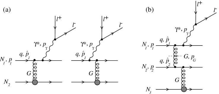
Figure 32: Diagrams for the two mechanisms for $l^{+}l^{-}$ production considered in this paper. (a) Dilepton production in $N\!N$ collisions which can be viewed as bremsstrahlung in $qq$ scattering (light cone approach) or as gluonic Compton scattering ($Gq\rightarrow\gamma^{*}q$) from the gluon cloud of the second nucleon (parton approach). (b) Dileptons from prompt gluons $Gq\rightarrow\gamma^{*}q$, where the on-mass-shell gluon G (crossed by a dashed line) is produced in another $N\!N$ collision.

First we discuss the direct production of lepton pairs within the light cone approach, fig. 32a. We employed the older parametrization (152) from [13] in our calculations, which works very well at the low $M^{2}$ values we are interested in. The improvement (157) modifies the DCS only small $\rho$, corresponding to large virtuality, and will not alter the result. The partonic cross section (22) has to be embedded into the hadronic process. The cross section of direct ($D$) dilepton production in nucleon-nucleon ($N\!N$) takes the form

$$\frac{d^{2}\sigma^{D}_{N\!N}}{dMdy}=\frac{\alpha_{em}}{3\pi M}\sum_{f}e_{q}^{2}\int_{x_{1}}^{1}d\alpha\frac{x_{1}}{\alpha^{2}}\left[q_{f}\left(\frac{x_{1}}{\alpha}\right)+q_{\bar{f}}\left(\frac{x_{1}}{\alpha}\right)\right]\frac{d\sigma(qN\rightarrow\gamma^{*}qN)}{d(\ln\alpha)}\,+\,\Bigl{\{}y\Rightarrow-y\Bigr{\}},$$ (315)

where $y$ is the rapidity of the lepton pair in the c.m. frame and $x_{1}=(\sqrt{x_{F}^{2}+4M^{2}/s}+x_{F})/2$. The first term corresponds to radiation from the projectile quarks and the second term to radiation from the target quarks (see fig. 32a), which corresponds to replacement $y\to-y$ in the first term. Since the dominant contribution to the cross section comes from large values of $x_{1}/\alpha$, we neglect antiquarks in the projectile, $q_{\bar{f}}\left(x_{1}/\alpha\right)\equiv 0$. We parameterize the valence quark distribution in the form

$$q_{u}(x) = \frac{C_{u}}{\sqrt{x}}(1-x)^{3},$$ (316)

$$q_{d}(x) = \frac{C_{d}}{\sqrt{x}}(1-x)^{4},$$ (317)

where $C_{u,d}$ are defined by the normalization to the number of valence quarks $N_{u,d}$ in a nucleon

$$\int_{0}^{1}\!\!dx\,q_{u,d}(x)=N_{u,d}.$$ (318)

In the case of the proton-nucleus ($pA$) and nucleus-nucleus ($AB$) collisions the cross section of the direct production is given by the integration of the nuclear densities $\rho_{A,B}$ over the impact parameter

$$\frac{d^{2}\sigma{{}_{A\!B}^{D}}}{dMdy}=\int\!\!d^{2}b\int\!\!d^{2}s\int_{-\infty}^{\infty}\!\!dz_{A}\,\rho_{A}(\vec{s},z_{A})\int_{-\infty}^{\infty}\!\!dz_{B}\,\rho_{B}(\vec{b}\!-\!\vec{s},z_{B})\,\frac{d^{2}\sigma{{}_{N\!N}^{D}}}{dMdy}=AB\frac{d^{2}\sigma{{}_{N\!N}^{D}}}{dMdy}.$$ (319)

In this expression we neglect small shadowing effects. To obtain the rate of the dilepton events per interaction one has to divide expression (319) by the total cross section, which can be calculated using the Glauber expressions

$$\sigma_{pA} = \int d^{2}b\left[1-\exp\left(-\sigma^{in}_{N\!N}T_{A}(\vec{b})\right)\right],$$ (320)

$$\sigma_{AB} = \int d^{2}b\left[1-\exp\left(-\sigma^{in}_{N\!N}\int d^{2}s\,T_{A}(\vec{s})\,T_{B}(\vec{b}-\vec{s})\right)\right],$$ (321)

where $\sigma^{in}_{N\!N}\approx 30~{}{\rm mb}$ denotes the inelastic $N\!N$ cross section and we used the standard Woods-Saxon parameterization [190] for the nuclear density $\rho_{A,B}$ in

$$T_{A,B}(\vec{b})=\int^{\infty}_{-\infty}\!\!dz\,\rho_{A,B}(\vec{b},z).$$ (322)

There are still two sources of uncertainty:

• The dipole cross section $\sigma_{q\bar{q}}(s,\rho)$ cannot be calculated perturbatively at large transverse separations, which are important in the small mass region, however. We employ the phenomenological expression (152).

• The light-cone wavefunction $\Psi_{\gamma^{*}q}(\alpha,\rho)$ depends on the mass $m_{f}$ of the quark. To illustrate its influence we calculate the cross sections for the two extreme cases of the constituent quark mass $m_{f}=150$ MeV and $m_{f}=300$ MeV.

Our results for proton (p-Be, p-Au) and heavy ion (Pb-Au) scattering are shown in figs. 33,34 under the label “light cone”. The border lines of the shadowed areas correspond to different choices of the constituent mass $m_{f}$ ($150$ MeV and $300$ MeV for the upper and lower lines, respectively). We believe, that also a different dipole cross section cannot produce values, which are significantly out of the shaded area, because $\sigma_{q\bar{q}}$ is well constrained to describe the structure function $F_{2}$ and hadronic cross sections.

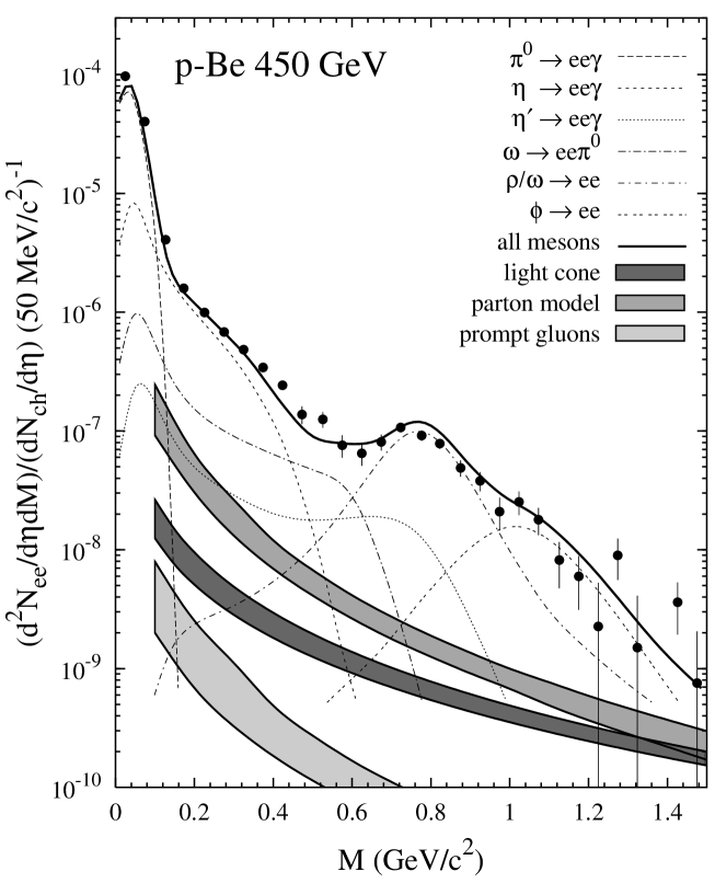
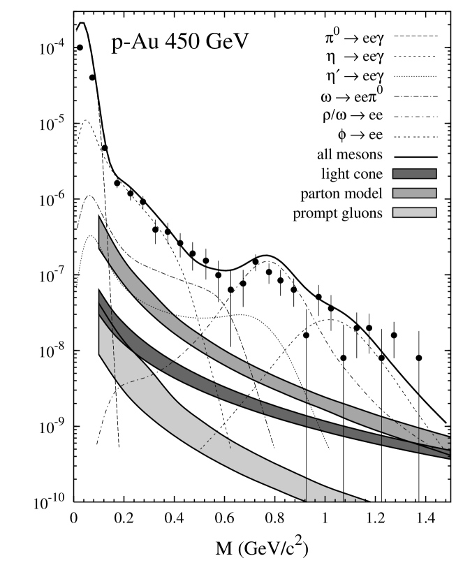
Figure 33: Data [171] on dilepton events in p-Be and p-Au scattering together with predictions from different mechanisms. The various curves correspond to meson decay channels. The shaded areas represent our results for direct production (in the light cone and the parton model approaches) and via prompt gluons: The upper limits correspond to the quark mass $m_{f}=150$ MeV and the lower ones to $m_{f}=300$ MeV. The curves for the parton model and for prompt gluons were calculated by Yu. Ivanov.

Figure 34: Data [172, 174] on dilepton events in Pb-Au scattering. The different curves correspond to meson decay channels. The shaded areas are our results for direct production in the light cone approach and via prompt gluons: the upper limits correspond to the quark mass $m_{f}=150$ MeV and the lower ones to $m_{f}=300$ MeV. Both processes contribute separately to the dilepton production and therefore their contributions have to be added. The curves for the parton model and for prompt gluons were calculated by Yu. Ivanov.

We compare these results with predictions of a parton model, which treats direct radiation of the lepton pair as Compton scattering of a target gluon on a beam quark (or vice versa) in pQCD. This formulation is in principle identical to the light-cone approach, but all nonperturbative and higher order effects which are parametrized in the DCS are not taken into account. The amplitude for the subprocess $qG\!\rightarrow\!l^{+}\!l^{-}\!X$ is well known and be found e.g. in [53]. The main uncertainties in this case originate from:

• Possible failure of pQCD calculations for the soft Compton amplitude.

• Poor knowledge of the gluon distribution function, especially at a soft scale.

We use the following gluon distribution function,

$$f_{G}(x)=\frac{C_{G}}{x^{1.1}}(1-x)^{5},$$ (323)

where $C_{G}$ is defined from the condition that gluons carry half of the nucleon momentum

$$\int_{0}^{1}\!\!dx\,x\,f_{G}(x)=\frac{1}{2}.$$ (324)

The results for proton (p-Be, p-Au) and heavy ion (Pb-Au) scattering are shown in figs. 33, 34. At low $M$ the results of pQCD (labeled as “parton model”) are higher than those from the light cone calculations but start to agree for $M\lower-1.93747pt\hbox{$>$}\kern-7.70004pt\lower 2.36806pt\hbox{$\sim$}1$ GeV. The reason for this is that the saturation of the dipole cross section becomes important at small $M$, and the cross section decays weaker than $1/M^{3}$. Although the parton model results are supposed to coincide with the predictions of the light-cone approach different approximations are used and the amount of disagreement between the results may serve as a measure of theoretical uncertainty. Nevertheless, we believe that light-cone prediction is more reliable.

The data in figs. 33 and 34 have been measured in a pseudorapidity interval of $2.1<\eta<2.65$, while our calculations have been performed for rapidity $y=2.4$. Note that the data are also subject to $p_{T}$ cuts, which exclude very small transverse momenta, $p_{T}<50$ MeV. These cuts are not included in our calculation. In the region of interest ($M=0.2$–$0.8$ GeV) however both approaches underestimate the experimental data by at least a factor of 10. We therefore believe, that also a more careful calculation would not change our results.

The pQCD calculation of the Compton amplitude is similar to that for an interaction with on mass shell gluons. The second process, labeled “prompt gluons”, considers gluons which are radiated in an elementary $N\!N$ collision and which convert into a virtual photon via gluonic Compton scattering on another nucleon. To estimate their contribution to the dilepton pair production we start with the elementary Compton subprocess $G\,q\rightarrow\gamma^{*}\,q$ (see the upper part of Fig. 32b where the on-mass-shell gluon is marked by a dashed line). To calculate the prompt gluon spectrum we use the perturbative evaluation for the cross section of gluon radiation [16]

$$\frac{d^{2}\sigma(q\!\rightarrow\!qG)}{d\alpha dk^{2}}=\frac{3\alpha_{s}C}{\pi}\frac{2m_{f}^{2}\alpha^{4}k^{2}+\left[1+(1-\alpha)^{2}\right](k^{4}+\alpha^{4}m_{f}^{4})}{\left(k^{2}+\alpha^{2}m_{f}^{2}\right)^{4}}\left[\alpha+\frac{9}{4}\frac{1-\alpha}{\alpha}\right],$$ (325)

where $k^{2}$ is the transverse momentum of the gluon, $C$ is the factor of the dipole approximation for the cross section of a $q\hat{q}$ pair with a nucleon (in this energy range $C\approx 3$ [161]) and $\alpha$ is the fraction of the quark light cone momentum carried by the gluon, as usual.

Finally, we combine the cross section for the elementary process with the distribution function $q_{f}(x_{1})$ for the quark and the distribution $dn_{G}/dx_{G}$ of the gluon to the cross section for the prompt (“P”) process on the nucleon

$$\frac{d^{2}\sigma{{}^{P}}}{dMdy}=\frac{d^{2}\sigma{{}^{P}_{+}}}{dMdy}+\frac{d^{2}\sigma{{}^{P}_{-}}}{dMdy},$$ (326)

with

$$\frac{d^{2}\sigma{{}^{P}_{+}}}{dMdy} = \sum_{f}\int_{0}^{1}\!\!dx_{1}q_{f}(x_{1})\int_{0}^{x_{G\,max}}\!\!dx_{G}\,\frac{dn_{G}}{dx_{G}}\,\frac{d^{2}\sigma{(qG\!\rightarrow\!l^{+}\!l^{-}\!X)}}{dMdy},$$ (327)

$$\frac{d^{2}\sigma{{}^{P}_{-}}}{dMdy} = \frac{d^{2}\sigma{{}^{P}_{+}}}{dMdy}\left(y\Rightarrow-y\right).$$ (328)

Here, $dn_{G}/dx_{G}$ is the gluon distribution over the longitudinal momentum fraction, the on mass shell gluon carries away from its parent quark, fig. 32. The calculations for the parton model and the prompt gluons were done by Yu. Ivanov and we refer to [187] for an expression for $dn_{G}/dx_{G}$ and for details of the calculation.

For nucleus-nucleus collisions the geometric factor has to take into account that points of gluon creation and interaction are different

$$\frac{d^{2}\sigma{{}_{A\!B}^{P}}}{dMdy} = \int\!\!d^{2}b\int\!\!d^{2}s\int_{-\infty}^{\infty}\!\!dz_{A}\,\rho_{A}(\vec{s},z_{A})\int_{-\infty}^{\infty}\!\!dz_{B}\,\rho_{B}(\vec{b}\!-\!\vec{s},z_{B})$$

$$\times \sigma^{in}_{N\!N}\,\left[\int_{-\infty}^{z_{A}}dz\rho_{A}(\vec{s},z)\frac{d^{2}\sigma{{}^{P}_{-}}}{dMdy}+\int_{z_{B}}^{\infty}dz\rho_{B}(\vec{b}\!-\!\vec{s},z)\frac{d^{2}\sigma{{}^{P}_{+}}}{dMdy}\right].$$

Again, expression (3.5) has to be divided by the total inelastic cross section to compare with experiment.

The results of our calculations are summarized in Figs. 33 and 34: the mechanisms considered contribute to the observed spectrum less than 10% and therefore are unimportant on the present level of discussion. On this level also the theoretical uncertainties, for instance in the choice of the value for constituent quark mass or in the evaluation via two mechanisms (light cone vs. parton model) are not yet of importance.

3.6 DY shadowing in proton-nucleus collisions

In section 2.6 we introduced the light-cone approach to the DY process at low $x_{2}$, in which DY dilepton production is viewed in the rest frame of the target and appears as bremsstrahlung from an incident quark. In the case of a nuclear target, this quark undergoes multiple rescatterings and in the simplest case radiates electromagnetic bremsstrahlung every time it is hit. As it is well known, this naive expectation is wrong at high energies. Landau and Pomeranchuk [17, 18] were the first who noticed that the cross section for bremsstrahlung of a high energetic charge in an amorphous medium is suppressed compared to the Bethe-Heitler cross section. Somewhat later, a quantum mechanical treatment of this effect, today known as the Landau-Pomeranchuk-Migdal (LPM) effect, was given by Migdal [19]. The LPM effect was measured recently at SLAC [21, 22, 23].

At low $x_{2}$, multiple rescattering of the quark inside the nucleus leads to an LPM suppression of bremsstrahlung from that quark. This suppression is the nuclear shadowing effect for the DY process, which was measured for the first time by the E772 collaboration [3].

What is the physical mechanism behind this suppression? The answer is that the quark needs a rather long time to recreate its electromagnetic field. This coherence time is related to the longitudinal momentum transfer by the uncertainty relation

$$l_{c}=\frac{1}{q_{L}}=\frac{\alpha(1-\alpha)E_{q}}{(1-\alpha)M^{2}+\alpha^{2}m_{f}^{2}+p_{T}^{2}},$$ (330)

where $E_{q}$ is the energy of the projectile quark. If the quark is hit again before it has recreated its field, it cannot radiate another photon. Note however that the Fourier modes of the field with high transverse momentum $p_{T}$ are recreated earlier as the one with low $p_{T}$. A large transverse momentum corresponds to a small size of the $\gamma^{*}q$-fluctuation. The small size fluctuation are therefore less shadowed. The low $p_{T}$ components of the field correspond to large $\gamma^{*}q$ fluctuations which are strongly shadowed.

Since the photon carries the momentum fraction $x_{1}$ away from the proton, the coherence length for DY can be written as

$$l_{c}=\frac{1}{m_{N}x_{2}}\frac{(1-\alpha)M^{2}}{(1-\alpha)M^{2}+\alpha^{2}m_{f}^{2}+p_{T}^{2}}.$$ (331)

The role of $x_{Bj}$ in DIS is played by $x_{2}$ in DY. One can define a mean coherence length for DY in analogy to the one for DIS, see section 3.4. We will however not pursue the concept of the mean coherence length for DY in this work. This has to be postponed to future studies. Like in low $x_{Bj}$ DIS, the coherence length for DY can become substantially longer than a nuclear radius.

In the case of an infinitely long coherence length $l_{c}\to\infty$, the whole target acts like a single scattering center and the partonic DY cross section can again be written, cf. (129), in factorized light-cone form

$$\frac{d\sigma^{qA}_{{T,L}}}{d\ln\alpha}=\int d^{2}\rho\,|\Psi^{T,L}_{\gamma^{*}q}(\alpha,\rho)|^{2}\Sigma_{q\bar{q}}(s,\alpha\rho),$$ (332)

where

$$\Sigma_{q\bar{q}}(s,\alpha\rho)=2\int d^{2}b\left(1-\exp\left(-\frac{\sigma_{q\bar{q}}(s,\alpha\rho)}{2}T(b)\right)\right)$$ (333)

is the eikonalized dipole cross section. One immediately sees that (332) is the analog of the eikonal formula for DIS (189). The eikonal term obviously leads to a reduction of the total cross section. It contains the LPM suppression. As already pointed out in section 3.1 for the case of shadowing in DIS, also (332) is different from the usual Glauber formula, where $\sigma_{q\bar{q}}(s,\alpha\rho)$ is averaged in the exponent.

In the case of a finite coherence length, which is relevant for all present and most of the future experiments, the DY cross section on the partonic level can be calculated with the same Green function technique as the DIS cross section [16]

$$\frac{d\sigma^{qA}_{{T,L}}}{d\ln\alpha} = A\,\frac{d\sigma^{qp}_{{T,L}}}{d\ln\alpha}\,-\,\frac{1}{2}{\rm Re}\int d^{2}b\int\limits_{-\infty}^{\infty}dz_{1}\int\limits_{z_{1}}^{\infty}dz_{2}\int d^{2}\rho_{1}\int d^{2}\rho_{2}\,$$ (334)

$$\times \Bigl{[}\Psi^{T,L}_{\gamma^{*}q}\left(\alpha,\rho_{2}\right)\Bigr{]}^{*}\,\rho_{A}\left(b,z_{2}\right)\sigma_{q\bar{q}}\left(s,\alpha\rho_{2}\right)G\left(\vec{\rho}_{2},z_{2}\,|\,\vec{\rho}_{1},z_{1}\right)$$

$$\times \rho_{A}\left(b,z_{1}\right)\sigma_{q\bar{q}}\left(s,\alpha\rho_{1}\right)\Psi^{T,L}_{{\gamma^{*}q}}\left(\alpha,\rho_{1}\right),$$

cf. section 3.2. The Green function $G$ fulfills a two dimensional Schrödinger equation, similar to (197),

$$\left[{\rm i}\frac{\partial}{\partial z_{2}}+\frac{\Delta_{\perp}\left(\rho_{2}\right)-\eta^{2}}{2E_{q}\alpha\left(1-\alpha\right)}+\frac{{\rm i}}{2}\rho_{A}\left(b,z_{2}\right)\,\sigma_{q\bar{q}}\left(s,\alpha\rho_{2}\right)\right]G\left(\vec{\rho}_{2},z_{2}\,|\,\vec{\rho}_{1},z_{1}\right)$$

$$={\rm i}\delta\left(z_{2}-z_{1}\right)\delta^{\left(2\right)}\left(\vec{\rho}_{2}-\vec{\rho}_{1}\right).$$ (335)

The two dimensional Laplacian in (335) acts on the transverse coordinate and takes into account that the quark is deflected due to the radiation process by a small, but non-zero angle. Note, that for convenience we included the phase factor $\exp(-{\rm i}q_{L}^{min}(z_{2}-z_{1}))$, describing the longitudinal motion, into the Green function $G$, ($q_{L}^{min}=\eta^{2}/2E_{q}\alpha\left(1-\alpha\right)$). This phase factor is not contained in $W$ and appears explicitly in (194). For a calculation that can be compared with experimental data, one has to embed the partonic cross section into the hadronic environment. For a proton as projectile, this is done in the same way as in (138),

$$\frac{d\sigma}{dM^{2}dx_{F}}=\frac{\alpha_{em}}{6\pi M^{2}}\frac{1}{x_{1}+x_{2}}\int_{x_{1}}^{1}\frac{d\alpha}{\alpha}F_{2}^{p}\left(\frac{x_{1}}{\alpha}\right)\frac{d\sigma(qp\to q\gamma^{*}p)}{d\ln\alpha}.$$

Given a parametrization of the proton structure function $F_{2}^{p}$, like the one from [125], one is in the position to calculate shadowing for the DY process. A comparison to experimental data will be presented in section 3.7. First we investigate the behavior of shadowing and find out, how much it will influence dilepton production at RHIC.

An analytical expression for the Green function $G$ can be obtained if one employs the approximation $\sigma_{q\bar{q}}(a,\alpha\rho)=C(s)\alpha^{2}\rho^{2}$ for the dipole cross section and a uniform nuclear density, cf. section 3.2. Such an approximation works remarkably, especially for heavy nuclei. Nevertheless, it can improved if one makes use of the fact that the asymptotic expression (332) is easily calculated with the realistic parametrization of the dipole cross section (157) and realistic nuclear density. One needs to use the full Green function only in the transition region from no-shadowing to a fully developed shadowing given by (332). Therefore, the value of the uniform nuclear density is fixed by demanding that the asymptotic shadowing ratio is the same for the realistic Woods-Saxon form of the nuclear density [190] and for the effective uniform density $\rho_{0}$. We have checked that the found value of $\rho_{0}$ is practically independent of the value of the cross section in the interval $1-50$ mb. The factor $C(s)$ is fixed in the same way, but now separately for transverse and longitudinal photons and for each value of $\alpha$. All further analytical calculations are similar to the one performed for shadowing in DIS, see appendix A.4.

Figure 35: The dependence of shadowing in proton-nucleus collisions for the DY process on $x_{F}$ for FNAL (E772) ($\sqrt{S}=38.8$ GeV) and RHIC ($\sqrt{S}=200$ GeV) energies. The calculations are for tungsten. Both curves are calculated for $M=5$ GeV and show the same points as in fig. 36. At RHIC, the whole $x_{F}$-range is shadowed.

Figure 36: The dependence of shadowing in proton-nucleus collisions for the DY process on $x_{2}$. The curves show the same points as fig. 35. The calculations are for tungsten. Much lower values of $x_{2}$ are reached at RHIC than at FNAL.

Our predictions for RHIC are depicted in figs. 36 and 35 in comparison with a curve calculated at the highest energy that can be reached today at FNAL. ISR at CERN can actually reach higher energies, $\sqrt{S}=62$ GeV, but did never include nuclei nor performed measurements at low $x_{2}$. The curves in the two figures show the same points, but in one figure, 36, displayed vs. $x_{2}$ and in the other figure, 35, vs. Feynman $x_{F}$. Shadowing in DY is more complicated than in DIS, because there a two structure function, of the projectile and of the target, involved in DY. Calculations are performed only for values of $x_{F}>0.1$, because at smaller values quarks from the target will also radiate in the same direction, which is not taken into account in (3.6).

One immediately recognizes that RHIC can reach much lower values of $x_{2}$ than FNAL. Even more striking, the whole $x_{F}$ range at RHIC shows strong shadowing. This illustrates the close connection between heavy ion collisions at high energies and low $x$ physics. The physics at RHIC is governed by coherence effects. The situation is different at SpS, where the energy is not high enough to allow for strong coherence effects. For a reliable interpretation of the data from RHIC and LHC it is essential to have good theoretical understanding of shadowing effects, because DY dilepton serve as a reference for the study of heavy quarkonium suppression, esp. $J/\psi$, which is believed to be a signal for quark gluon plasma formation [189].

It is also interesting to investigate the influence of the nuclear medium on the transverse momentum distribution of the DY pairs. The formula for the differential cross section was derived in [16]. It reads,

$$\frac{d^{3}\sigma^{qA}}{d(\ln\alpha)d^{2}p_{T}} = \frac{\alpha_{em}}{(2\pi)^{4}4E_{q}^{2}(1-\alpha)^{2}}2{\rm Re}\int_{-\infty}^{\infty}dz_{1}\int_{z_{1}}^{\infty}dz_{2}\int d^{2}b\,d^{2}k_{T}\,d^{2}\rho_{1}\,d^{2}\rho_{2}$$ (336)

$$\times \exp\left[{\rm i}\alpha\vec{p}_{2}\cdot\vec{\rho}_{2}-{\rm i}\alpha\vec{p}_{1}\cdot\vec{\rho}_{1}-{\rm i}\int\limits_{z_{2}}^{\infty}dzV_{opt}(b,\rho_{2},z)-{\rm i}\int\limits_{-\infty}^{z_{1}}dzV_{opt}(b,\rho_{1},z)\right]$$

$$\times \left[\widehat{\cal O}_{\gamma^{*}q}(\vec{\rho}_{2})\right]^{*}\widehat{\cal O}_{\gamma^{*}q}(\vec{\rho}_{1})G\left(\vec{\rho}_{2},z_{2}\,|\,\vec{\rho}_{1},z_{1}\right),$$

where $k_{T}$ is the transverse momentum of the quark in the final state. It is convenient to introduce the transverse momenta relative to the direction of the virtual photon. The transverse momentum of the incoming quark relative to this direction is then given by

$$\vec{p}_{1}=\frac{\vec{p}_{T}}{\alpha}$$ (337)

and the transverse momentum of the final quark by

$$\vec{p}_{2}=\vec{k}_{T}-\frac{1-\alpha}{\alpha}\vec{p}_{T}.$$ (338)

The interaction with the nuclear medium is contained in the Green function $G$, which fulfills the two dimensional Schrödinger equation (335) and in the optical potential

$$V_{opt}(b,\rho,z)=-\frac{{\rm i}}{2}\rho_{A}(b,z)\sigma_{q\bar{q}}(s,\rho).$$ (339)

This potential describes the shadowing corrections and is also present in (335). The operators $\widehat{\cal O}$, acting on the variable $\vec{\rho}_{1}$ or $\vec{\rho}_{2}$ in the Green function $G$ in (336), are given by (132) and (133). They are the same operators which appear in the definition of the LC wavefunctions for the transition $q\to\gamma^{*}q$, cf. section 2.6. It has been shown in [16], that in the limit of infinitely high energy of the incoming quark, $E_{q}\to\infty$, the differential cross section (336) takes an eikonal form, similar to (146),

$$\frac{d\sigma(qp\to q\gamma^{*}p)}{d\ln\alpha d^{2}p_{T}} = \frac{1}{(2\pi)^{2}}\int d^{2}\rho_{1}d^{2}\rho_{2}\,\exp[{\rm i}\vec{p}_{T}\cdot(\vec{\rho}_{1}-\vec{\rho}_{2})]\Psi^{*}_{\gamma^{*}q}(\alpha,\vec{\rho}_{1})\Psi_{\gamma^{*}q}(\alpha,\vec{\rho}_{2})$$ (340)

$$\times \frac{1}{2}\left\{\Sigma_{q\bar{q}}(\alpha\rho_{1})+\Sigma_{q\bar{q}}(\alpha\rho_{2})-\Sigma_{q\bar{q}}(\alpha(\vec{\rho}_{1}-\vec{\rho}_{2}))\right\},$$

where $\Sigma_{q\bar{q}}$ is given by (333).

Figure 37: The transverse momentum dependence of the LPM effect for different energies. The curves are for tungsten and $M=5$ GeV, $x_{F}=0.7$. an approximate dipole cross section $\sigma_{q\bar{q}}(s,\rho)=C(s)\rho^{2}$ is used.

The transverse momentum dependence of the LPM effect, calculated from (336), is depicted in fig. 37. The calculations are for tungsten. The mass of the lepton pair is $M=5$ GeV and Feynman $x_{F}=0.7$. Since (336) is very complicated, the following simplifying approximations are employed. First, a uniform nuclear density of $\rho_{A}=0.16$ fm^-3 is used, which is well justified for a heavy nucleus like tungsten, and second, the approximation $\sigma_{q\bar{q}}(s,\rho)=C(s)\rho^{2}$ is applied. The latter approximation works remarkably well, especially for heavy nuclei [153]. With these approximations, some of the 12 integrations in (336) can be performed analytically. The result of the analytical calculations is given in appendix A.3. One further integration has to be performed, in order to account for the hadronic environment, cf. (149). To make the calculations even more realistic, an energy dependence of the factor $C(s)$ is introduced. At FNAL energies, a value of $C(\sqrt{s}=38.8~{}{\rm GeV})=3$ is appropriate, while at RHIC energies one rather has $C(\sqrt{s}=200~{}{\rm GeV})=6$.

Note that pairs with low transverse momenta are suppressed at small $p_{T}\leq 1$ GeV, but enhanced at $p_{T}\geq 1$ GeV. This enhancement in the intermediate $p_{T}$ region is already known for a long time as Cronin-effect [191]. It is usually assumed that the Cronin-effect is caused by multiple scatterings and the light-cone approach reproduces this phenomenon. At very large $p_{T}$, all nuclear effects vanish. Furthermore, the shadowing at small $p_{T}$ increases with energy, since the dipole cros section becomes larger.

Although (336) looks rather complicated, it contains intuitively understandable physics. The nucleus acts as a color filter [5]. Small size dipoles, having large $p_{T}$, can pass the nucleus nearly undisturbed while dileptons with small transverse momentum are shadowed, because they correspond to large arguments $\rho$ of the dipole cross section. Note that (336) contains also the phenomenon of nuclear broadening. Due to multiple rescatterings, the projectile quark performs a random walk in impact parameter space, while propagating through the nucleus. Therefore, not the whole suppression at small $p_{T}$ is due to nuclear shadowing. Part of the dileptons reappear at larger transverse momentum, which leads to the enhancement in the intermediate $p_{T}$ region. Indeed, it was found in [192], that in the approximation $\sigma_{q\bar{q}}(s,\rho)=C\rho^{2}$, the transverse momentum broadening is given by

$$\delta\langle p_{T}\rangle^{pA}=\langle p_{T}\rangle^{pA}-\langle p_{T}\rangle^{pp}=C\langle T(b)\rangle,$$ (341)

where $\langle T(b)\rangle=\int d^{2}bT^{2}(b)/A$, is the mean nuclear thickness.

First numerical calculation with the eikonal approximation (340) are performed in [16], but only for quark-nucleus scattering. Our results are consistent with the one from [16]. Note that the transverse momentum dependence of the LPM effect in QED is also investigated in [40]. The case of gluon radiation off a quark is studied in [193, 194].

Recently, also the approach by Luo, Qiu and Sterman [69, 70] has received much attention, see e. g. [195]-[198]. This approach extends the QCD factorization theorem [199] to higher twist operators. The double scattering contribution to the DY process is described in terms of a matrix element, which contains all the nonperturbative physics, and a hard part that can be calculated in perturbation theory. However, it was already mentioned in section 2.5 that the calculation of the transverse momentum distribution is very complicated in pQCD, since it requires the resummation of large logarithms $\ln(p_{T}^{2}/M^{2})$ at $p_{T}^{2}\ll M^{2}$. It is known, how to perform this resummation for the leading twist [121, 122, 123], but it still has to be investigated, how these techniques can be generalized to higher twists.

3.7 Comparison with data

The mean coherence length introduced in section 3.4 alone is not sufficient to predict any nuclear effect in the structure function $F_{2}$. It is merely intended to be a tool for qualitative considerations. The Green function technique from section 3.2 does not need the mean coherence length as input. Instead, all coherence effects are automatically taken into account by the Green function (197). Together with a realistic phenomenological dipole cross section we are now able to perform parameter free calculations for nuclear shadowing in the region which is most difficult for theory: The transition region between no shadowing at $x_{Bj}\sim 0.1$ and saturated (for the $|{q\bar{q}}\rangle$ component) shadowing at very small $x_{Bj}$.

In the rest frame of the nucleus shadowing in the total virtual photoabsorption cross section $\sigma^{\gamma^{*}A}_{tot}$ (or in the structure function $F_{2}^{A}$) can be decomposed over different Fock components of the photon,

$$\sigma_{tot}^{\gamma^{*}A}=A\,\sigma_{tot}^{\gamma^{*}p}\,-\,\Delta\sigma_{tot}({q\bar{q}})\,-\,\Delta\sigma_{tot}({q\bar{q}}G)\,-\,\Delta\sigma_{tot}({q\bar{q}}2G)\,-\,...$$ (342)

It was found in section 3.4 that the coherence length for the $|q\bar{q}G\rangle$ fluctuation is rather short at $x_{Bj}\sim 0.01$, compared to the mean internucleon spacing in a nucleus, because of it’s large mass, see fig. 29. Although the calculations were done only at large $Q^{2}$ and some data are at quite small $Q^{2}$, we neglect the $|q\bar{q}G\rangle$ component of the virtual photon for the present comparison with data. It is one of the most important tasks for the future, to include also the gluon, since it is important for shadowing of the nuclear gluon distribution. The treatment of the propagation of the three body system $q\bar{q}G$ through the nucleus is however numerically quite involved.

Holding only the first two terms on the r.h.s. of (342), the total cross section for transverse and longitudinal photons on a nucleus can be represented as

$$\sigma^{\gamma^{*}A}_{{T,L}} = A\,\sigma^{\gamma^{*}p}_{{T,L}}\,-\,\frac{1}{2}{\rm Re}\int d^{2}b\int\limits_{0}^{1}d\alpha\int\limits_{-\infty}^{\infty}dz_{1}\int\limits_{z_{1}}^{\infty}dz_{2}\int d^{2}\rho_{1}\int d^{2}\rho_{2}\,$$ (343)

$$\times \Bigl{[}\Psi^{T,L}_{{q\bar{q}}}\left(\varepsilon,\lambda,\rho_{2}\right)\Bigr{]}^{*}\,\rho_{A}\left(b,z_{2}\right)\sigma_{q\bar{q}}\left(s,\rho_{2}\right)G\left(\vec{\rho}_{2},z_{2}\,|\,\vec{\rho}_{1},z_{1}\right)$$

$$\times \rho_{A}\left(b,z_{1}\right)\sigma_{q\bar{q}}\left(s,\rho_{1}\right)\Psi^{T,L}_{{q\bar{q}}}\left(\varepsilon,\lambda,\rho_{1}\right),$$

where $\rho_{A}(b,z)$ is the nuclear density dependent on impact parameter $b$ and longitudinal coordinate $z$. In (343) we have generalized our result from section 3.2 to include also the nonperturbative interaction proposed in [13], see also section 2.3. The nonperturbative wave functions for the ${q\bar{q}}$ component of the photon are defined in (2.3)-(78). The Green function $G\left(\vec{\rho}_{2},z_{2}\,|\,\vec{\rho}_{1},z_{1}\right)$ describes propagation of a nonperturbatively interacting ${q\bar{q}}$ pair in an absorptive medium. It fulfills the two dimensional Schrödinger-equation,

$$\left[{\rm i}\frac{\partial}{\partial z_{2}}+\frac{\Delta_{\perp}\left(\rho_{2}\right)-\varepsilon^{2}}{2\nu\alpha\left(1-\alpha\right)}+\frac{{\rm i}}{2}\rho_{A}\left(b,z_{2}\right)\,\sigma_{q\bar{q}}\left(s,\rho_{2}\right)-\frac{a^{4}\left(\alpha\right)\rho_{2}^{2}}{2\nu\alpha\left(1-\alpha\right)}\right]G\left(\vec{\rho}_{2},z_{2}\,|\,\vec{\rho}_{1},z_{1}\right)$$

$$={\rm i}\delta\left(z_{2}-z_{1}\right)\delta^{\left(2\right)}\left(\vec{\rho}_{2}-\vec{\rho}_{1}\right)\ ,$$ (344)

where $a(\alpha)$ and $\lambda$ are given by (76) and (81) respectively. The third term on the l.h.s. of (344) describes the absorption of a ${q\bar{q}}$ pair with cross section $\sigma_{{q\bar{q}}}\left(s,r\right)$ in the medium of density $\rho_{A}\left(b,z\right)$. Note that the Green function $G$ includes now also the motion in longitudinal direction, in contrast to the Green function $W$ in (197). The longitudinal motion is contained in the term $\varepsilon^{2}/2\nu\alpha\left(1-\alpha\right)$ in (344).

An explicit analytical expression for $W$ can be found only for a dipole cross section $\sigma_{{q\bar{q}}}(s,\rho)=C(s)\rho^{2}$ and a constant nuclear density $\rho_{A}(b,z)=\rho_{0}$. Such an approximation has a reasonable accuracy, especially for heavy nuclei. Nevertheless, it can be even more precise if one makes use of the fact that the asymptotic expression (189) is easily calculated with the realistic parametrization of the dipole cross section (157) and a realistic nuclear density. One needs the full Green function only in the transition region from no-shadowing to a fully developed shadowing given by (189). Therefore, we fix the value of the uniform nuclear density by demanding that the asymptotic shadowing ratio is the same for the realistic Woods-Saxon form of the nuclear density [190] and for the effective uniform density $\rho_{0}$. We checked that the found value of $\rho_{0}$ is practically independent of the value of the cross section in the interval $1-50$ mb. The factor $C$ is fixed in the same way, but now separately for transverse and longitudinal photons and for each value of $\alpha$. More details can be found in appendix A.4.

We perform calculations with the parameter $v$ in (76) fixed at $v=0.5$, because the parameters in the dipole cross section are fixed for this value of $v$, see section 2.7. The dependence on $v$ is very weak. All calculations are also performed with perturbative wavefunctions (45, 46) and the quark masses given on page 162. The results are shown in figs. 38-42. Curves obtained with nonperturbative wavefunctions are drawn with solid lines and the results from perturbative wavefunctions are depicted by dashes lines. The calculations are for the same kinematics as the datapoints. We neglect shadowing in the deuterium structure function $F_{2}^{D}$, which is of order $\leq 5$% [200]. The antishadowing effect which occurs at $x_{Bj}\sim 0.1$ is neglected as well. Shadowing is calculated only for nuclei with $A\geq 12$, since the basic formula is derived in the approximation $A\gg 1$. Although the calculations are parameter free, agreement is reasonably good.

Fig. 38 shows a comparison of the calculations with experimental data for the structure function ratios of carbon and calcium over deuterium from NMC [201, 202]. Unlike other NMC data, these data reach down to quite small $x_{Bj}$, where the error bars for carbon are quite large. At the last point in the carbon plot, the solid curve turns unexpectedly upwards. No such behavior is visible in the perturbative calculation. Note, that the data are at different values of $Q^{2}$. The leftmost point has $Q^{2}=0.035$ GeV² and the rightmost point $Q^{2}=9.6$ GeV². Because of the very small $Q^{2}$ of the point at the lowest value of $x_{Bj}$, we attribute the decrease of shadowing to the model of the nonperturbative interaction. The calcium data and part of the carbon data shown in this figure are the result of a reevaluation of the data from [203, 204]. Among other reasons, the reevaluation was necessary, because the radiative corrections require knowledge of $F_{2}^{D}$ over a large range of $x_{Bj}$ and $Q^{2}$. When new information about $F_{2}^{D}$ became available from SLAC, the radiative corrections were performed again [201]. This lead to an increase of the structure function ratio by at most 2.5% for Ca/D at the lowest value of $x_{Bj}$ [201].

In fig. 39, we compare our calculation to NMC data from [162, 201] for different nuclei, ranging from aluminium to lead measured relative to carbon. Shadowing is always slightly larger in the nonperturbative calculation. This is in accordance with the observation in section 2.7 that the choice of the quark mass squeezes the wavepacket somewhat more than the nonperturbative interaction. Since shadowing is determined by diffraction, which is an almost entirely soft process, one is more sensitive to the large $\rho$ behavior of the dipole cross section and to details of the nonperturbative interaction. The perturbative calculation seems to reproduce the data better than the nonperturbative. Note however that taking into account the antishadowing effect would shift the curves upwards. Whether this will happen at all values of $x_{Bj}$ or only around $x_{Bj}\sim 0.1$ is model dependent. We prefer not to introduce new parameters. Note that the data in fig. 39 correspond to different muon beam energies, $90$ GeV for the calcium data in the upper row and $200$ GeV for all other data. The structure function ratio is however independent of the beam energy. Indeed one sees from the equations in section 2.1 that

$$\frac{F_{2}^{A}}{F_{2}^{D}}=\frac{\sigma_{T}^{\gamma^{*}A}+\sigma_{L}^{\gamma^{*}A}}{\sigma_{T}^{\gamma^{*}D}+\sigma_{L}^{\gamma^{*}D}},$$ (345)

while for the measured lepton-target cross section one has

$$\frac{\sigma^{lA}}{\sigma^{lD}}=\frac{F_{2}^{A}}{F_{2}^{D}}\frac{(1+\epsilon R_{A})(1+R_{D})}{(1+R_{A})(1+\epsilon R_{D})},$$ (346)

where

$$\epsilon=\frac{4(1-y)-\frac{4m_{N}^{2}x_{Bj}^{2}}{Q^{2}}}{4(1-y)+2y^{2}+\frac{4m_{N}^{2}x_{Bj}^{2}}{Q^{2}}}$$ (347)

is the photon polarization parameter and

$$R_{A}=\frac{\left(1+\frac{4m_{N}^{2}x_{Bj}^{2}}{Q^{2}}\right)\sigma_{L}^{\gamma^{*}A}+\frac{4m_{N}^{2}x_{Bj}^{2}}{Q^{2}}\sigma_{T}^{\gamma^{*}A}}{\sigma_{T}^{\gamma^{*}A}}\approx\frac{\sigma_{L}^{\gamma^{*}A}}{\sigma_{T}^{\gamma^{*}A}}.$$ (348)

The lepton nucleon cross section ratio is only equal to the structure function ratio, if there are no nuclear effects in $R$. This is assumed in all NMC data and supported by experimental observations. In the kinematical region relevant for NMC, $R$ data show practically no $A$ dependence [205].

The best data available today for nuclear shadowing in DIS are for the structure function ratio Sn/C from NMC [206]. These are shown in figs. 40 and 41. Although our calculation describes the existing data quite well, the dip in the $Q^{2}$ dependence of the solid curve in fig. 41 looks rather suspicious. This dip is practically invisible if one employs the older parametrization (152) of the dipole cross section [207]. It is therefore caused by the suppression factor in the improved parametrization (157). Since the dip is not present in the perturbative calculation, it is also related to the nonperturbative interaction. We do not believe that this indicates a physical effect. One rather has to improve the dipole cross section and the nonperturbative interaction, in order to get a better description of the $Q^{2}$ dependence of shadowing. We also hope to overcome the numerical prescription we use for the dipole cross section in the future and to perform the calculations with the exact parametrization.

We also compare our parameter free calculations to data from E665 [208, 209], where much lower values of $x_{Bj}$ are covered, fig. 42. The decrease of shadowing in the solid curve at very low $x_{Bj}$ and $Q^{2}$, which was already visible in fig. 38, is also seen in the Xe/D plot. The agreement with data is less good for the E665 data than for the NMC data. Indeed, the two datasets contradict each other [162, 205] and no calculation can reproduce both. The disagreement between NMC and E665 vanishes however, in the $F_{2}$ ratio relative to carbon. Note also that the $q\bar{q}G$ component will become important at very low $x_{Bj}$ and calculations, taking only the $q\bar{q}$ state into account, will be unreliable at $x_{Bj}\ll 0.01$.

Besides describing all data reasonably well, the success of the Green function technique is to reproduce the correct shape of the curves vs. $x_{Bj}$. Without treating the coherence length properly, shadowing would set in quite abruptly at $x_{Bj}\sim 0.1$ and quickly saturate as one goes to lower $x_{Bj}$, cf. fig. 28.

Nuclear shadowing is very challenging from the experimental point of view, because of large radiative corrections. These corrections occur, e.g. when the incident lepton, see fig. 3, radiates bremsstrahlung and does not produce a deep inelastic event [90]. In the older publications [203, 204], the NM collaboration calculated the radiative corrections employing the computer program FERRAD, which relies on the theoretical analysis by Mo and Tsai [215]. For the reevaluation of the shadowing data [201] three different codes were tested, FERRAD, an improved version of FERRAD and TERAD. The latter relies on the work of Akhundov, Bardin, and Shumeiko [210, 211, 212] and was used for the published NMC result. A more detailed discussion on radiative corrections for NMC and HERMES can be found in [213]. We point out that the whole shadowing effect in the data shown in figs. 38-41 is calculated. Without radiative corrections, the cross section ratio would be around unity [213, 216]. However, the correctness of the calculation was checked by comparing to the ”hadron tagged” data, making sure that really a deep inelastic event was measured.

A different way to identify the deep inelastic events was chosen by the E665 collaboration [208, 209], where cuts in the electromagnetic calorimeter were applied. In [208] the xenon data obtained in this way were compared to an evaluation with hadron tagging, see fig. 42. The two methods give consistent results. In [209], the E665 collaboration also applied the FERRAD code for a comparison with NMC. The results are depicted by open circles in fig. 42. The code wass assumed to be reliable only in the region $y<0.7$, see (6), and $x_{Bj}>0.002$ [209]. Therefore it was not applied to all data points, but only to those, where it was supposed to work. One recognizes a systematic discrepancy between the two evaluation methods. The radiative corrected cross section ratios are lower by $\sim$5% than the points from the calorimeter analysis. We argue however from the date of the publication that the improved input for FERRAD used in [201] was not taken into account by E665 in [209]. It is of course impossible for the author to conclude which experiment is correct.

Figure 38: Comparison between calculations for shadowing in DIS and experimental data from NMC [201, 202] for the structure functions of carbon and calcium relative to deuterium. The $x_{Bj}$-dependence of shadowing is shown. The leftmost point of the carbon data is measured at $Q^{2}=0.035$ GeV² and the rightmost point at $Q^{2}=9.6$ GeV². The $Q^{2}$ values for calcium are $0.6~{}{\rm GeV}^{2}\leq Q^{2}\leq 9.7~{}{\rm GeV}^{2}$. The inner error bars show the statistical error and the outer error bars statistical and systematic error added in quadrature. The full curves are calculated with the Green function method (343) including the nonperturbative interaction. The dashed curves are calculated with the perturbative wavefunctions (45,46).

Figure 39: Comparison between calculations for shadowing in DIS and experimental data from NMC [162, 201] for the structure functions of different nuclei relative to carbon. The $x_{Bj}$-dependence of shadowing is shown. The $Q^{2}$ range covered by the data is approximately $3~{}{\rm GeV}^{2}\leq Q^{2}\leq 17~{}{\rm GeV}^{2}$ from the lowest to the highest $x_{Bj}$ bin. The different curves and error bars have the same meaning as in fig. 38.

Figure 40: The $x_{Bj}$ dependence of nuclear shadowing in DIS for the structure function ratio of tin relative to carbon. The data are from NMC [206]. The different curves and error bars have the same meaning as in fig. 38.

Figure 41: The $Q^{2}$ dependence of nuclear shadowing in DIS for the structure function ratio of tin relative to carbon. The data points [206] are the same as shown in fig. 40. The different curves and error bars have the same meaning as in fig. 38.

Figure 42: The $x_{Bj}$ dependence of nuclear shadowing in DIS for various nuclei. The data are from E665 [208, 209]. Full circles show data taken with electromagnetic calorimeter cuts, while the open circles result from the FERRAD radiative correction code. Hadronic cuts were applied for the triangles in the lower left plot. For better visibility, triangles and open circles are displaced to slightly lower $x_{Bj}$. The $Q^{2}$ range of the data is $0.15~{}{\rm GeV}^{2}\leq Q^{2}\leq~{}22.5~{}{\rm GeV}^{2}$, except for the xenon data, $0.03~{}{\rm GeV}^{2}\leq Q^{2}\leq 17.9~{}{\rm GeV}^{2}$, from the lowest to the highest value of $x_{Bj}$. The meaning of the different curves and error bars is explained below fig. 38.

Figure 43: The left figure shows the leptonic cross section ratio measured by HERMES for helium and nitrogen. The data are not at variance with other experiments, since the points correspond to different values of $Q^{2}$. The large enhancement in the $R$-ratio is shown on the right, $R_{A}=\sigma_{L}^{\gamma^{*}A}/\sigma_{T}^{\gamma^{*}A}$ The figures are from [214].

Much attention has been drawn to a possible $A$ dependence of $R$ and the importance of radiative corrections by the data released recently by the HERMES collaboration [214]. HERMES measured nuclear shadowing in DIS at the same values of $x_{Bj}$ as NMC, but at smaller virtuality, $0.5~{}{\rm GeV}^{2}\leq Q^{2}\leq 2.018~{}{\rm GeV}^{2}$ and larger $y<0.85$ (6). The $27.5$ GeV positron beam at HERA was used. The results shown in fig. 43, expose several striking features. The cross section ratio for nitrogen to deuterium is suppressed much stronger than it would have been expected extrapolating previous NMC measurements. This ratio is related to the $F_{2}$ ratio by (346). The two quantities are equal, only when $\epsilon=1$ or when there are no nuclear effects in $R$ (348). Since NMC could not find any nuclear effects in $R$, all NMC data were evaluated assuming $R_{A}=R_{D}$. Note that at HERMES $\epsilon\sim 0.4$ at low $x_{Bj}$. The discrepancy in the left part of fig. 43, can be interpreted in terms of different shadowing for transverse and longitudinal photons. It was concluded in [214] that while $\sigma_{L}$ is enhanced, $\sigma_{T}$ is suppressed on nitrogen by at least factor of two compared to a deuterium target. Then one obtains a structure function ratio of the same order of magnitude as observed before, fig. 44.

Figure 44: The $F_{2}$ ratio for nitrogen to deuterium measured by HERMES [214] compared calculations with the Green function method (343). The full curve is calculated with nonperturbative and the dashed curves with perturbative wavefunctions. The $Q^{2}$ range of the data is $0.5~{}{\rm GeV}^{2}\leq Q^{2}\leq 2.018~{}{\rm GeV}^{2}$.

Radiative corrections are huge at HERMES, because the positron mass is much smaller than the muon mass and because radiative corrections become very large at $y\to 1$ [90]. Furthermore, $F_{2}$ and $R$ are needed as input to calculate the radiative corrections and have to be known over a wide range of $x_{Bj}$ and $Q^{2}$. Therefore an iterative procedure was applied by HERMES [213, 214], using existing data as input to calculate the radiatively corrected cross sections in a first approximation. The new structure function and the new $R$ obtained in this way were again used as input to the computer program. This was repeated until convergence is obtained. To make the result reliable, three different codes were compared, FERRAD [215], TERAD [210, 211, 212] and POLRAD [217]. In spite of the statement in [209] that FERRAD is not applicable for $y>0.7$, all codes gave the same result within 2%. More details can be found in [213].

The HERMES experiment drew attention to the fact that only very few data are available in this kinematical region. Moreover, no reliable theoretical calculations are done yet. Approaches based on QCD evolution equations need parton distributions at a semi hard scale as input and their applicability is doubtful at the low $Q^{2}$ values of HERMES. More promising is the intuitive approach treating nuclear effects in the spirit of vector dominance model (VDM) [148] as shadowing for the total cross section of hadronic fluctuations of the virtual photon (see e. g.  [141]). However, the VDM is sensible only at small $Q^{2}\to 0$ not so easily generalized to longitudinal photons.

Eventually we are able to provide theoretical predictions from the light-cone approach, since nonperturbative effects are assumed to be parametrized in the dipole cross section and we also included the nonperturbative interaction introduced in [13] between the $q$ and the $\bar{q}$ for a more realistic description of the soft physics. The results of our calculations for the nitrogen $F_{2}$-ratio is shown in fig. 44 in comparison with HERMES data. We expect somewhat larger shadowing for $F_{2}$ than seen by HERMES.

Figure 45: The result of calculations in the light-cone approach compared to the HERMES measurement [214] of $R_{N}/R_{D}$. The data points are for the same kinematics as those shown in fig. 44. On this scale, the lines corresponding to perturbative (dashed) and nonperturbative (solid) wavefunctions lie on top of each other and predict an $R$-ratio of practically unity. The large enhancement for $\sigma_{L}^{\gamma^{*}N}$ measured by HERMES is clearly not reproduced in the light-cone approach.

The most striking feature of the HERMES data for shadowing is a dramatically rising $R=\sigma_{L}/\sigma_{T}$ ratio on nitrogen compared to proton target at $Q^{2}<1~{}{\rm GeV}^{2}$ [214]. Our predictions for $R_{N}/R_{p}$ are plotted in fig. 45 versus $Q^{2}$ at the same values of $x_{Bj}$ as the experimental points. Like in all other calculations, we neglect nuclear effects in deuterium. Apparently, we do not expect any remarkable effect. There is a priori no reason to think that the light-cone approach leads to equal shadowing for longitudinal and transverse photons. It is calculated in section 3.4 that the coherence length for longitudinal photons is significantly longer than for transverse. Apparently this is compensated by the smaller size of $q\bar{q}$-fluctuations from longitudinal photons, cf. section 2.3. One has however to bear in mind, that we can calculate shadowing for $\sigma_{L}$ only at small $Q^{2}$. In the approximation, when only the $q\bar{q}$ pair is taken into account, shadowing for longitudinal photons vanishes $\propto 1/Q^{2}$ at large $Q^{2}$. Taking also the $q\bar{q}G$ component into account, shadowing for $\sigma_{L}$ will persist at high $Q^{2}$, cf. section 2.4. We also calculated $R$ for a proton target and compared to NMC data [64] in the low $x_{Bj}$ region, fig. 46. Good agreement with the data is achieved over the whole $Q^{2}$ range, without introducing any new parameters. One might argue that the beginning of an increase of $R$ is visible from the low $Q^{2}$ points in fig. 46. There are however not enough data to allow for definite conclusions. Note that nuclear effects for $R$ were estimated previously in a different approach [220, 221].

Figure 46: The ratio of longitudinal to transverse cross section, $R=\sigma_{L}^{\gamma^{*}p}/\sigma_{T}^{\gamma^{*}p}$, for a proton measured by NMC [64]. The inner error bars represent the statistical error and the outer error bars statistical and systematic error added in quadrature. The full curve is calculated using nonperturbative and the dashed curves using perturbative wavefunctions. From the left to the right, the data are for the $x_{Bj}$ values $0.0080,~{}0.0045,~{}0.0125,~{}0.0175,~{}0.025,~{}0.035,~{}0.05,~{}0.07$, and $0.09$.

We suppose that our results provide a reliable base line for nuclear effects in this region. The dramatic effects revealed by the HERMES experiment probably cannot be explained without involving new nonstandard dynamics, see e.g. [222]. While a nuclear enhancement in the longitudinal cross section might be qualitatively explained by higher twist contributions, the enormous suppression for $\sigma_{T}$ which is implied by the $\sigma_{L}$ enhancement and fig. 43 still remains. Indeed, for the two leftmost points in fig. 45, one finds [213] $\sigma_{T}^{\gamma^{*}N}/\sigma_{T}^{\gamma^{*}p}\sim 0.45$. For nitrogen, this implies that the virtual photon splits up into something that interacts with an effective cross section of $\sim 100$ mb, compared to the usual $\sim 25$ mb for real photons and for $Q^{2}>1$ GeV².

Experimental data for shadowing in DY are available from the collaborations E772 [3] and E866 [218]. We compare only to the E772 data, although even smaller values of $x_{2}$ could be reached by the E866/NuSea collaboration. The latter measured however relative to a beryllium target. The large $A$ approximation and the uniform nuclear density we have to apply is not justified for such a light nucleus. These simplifications are necessary, because of merely technical difficulties and are not demanded by the nature of the light-cone approach, section 3.6. The result of the calculation, shown in fig. 47, agrees well with the data.

Practically all DY data are taken at masses $M$ higher than the $J/\psi$ mass, because of the large underground of dileptons from other sources at small $M^{2}$. It is therefore impossible to reach values of $x_{2}$ as low as the values of $x_{Bj}$ in the E665 data, fig. 42, at present. This situation will however change in the nearest future, when RHIC starts operating. With PHENIX, values of $x_{2}\sim 0.001$ and $M\sim 2$ GeV can be reached [219].

Figure 47: Comparison between calculations in the light-cone approach and E772 data [3] for shadowing in DY. Only perturbative wavefunctions are applied, since there is no real dipole in DY. The calculations are performed at the mean values of the lepton pair mass. From the left to the right, these values are $5$ GeV², $5.7$ GeV², and $6.5$ GeV².

4 Summary and outlook

In this work a phenomenological approach to nuclear shadowing in DIS and DY in the target rest frame is developed. As it is well known, the partonic interpretation of high energy scattering processes depends on the reference frame. In a frame, where the target is fast moving, DIS looks like the scattering of virtual photons off sea quarks in the target (at low $x_{Bj}$). In contrast to this, in the rest frame of the target the virtual photon splits up into a $q\bar{q}$-pair which then scatters off the target gluon field, see fig. 1. Note that in the infinite momentum frame the $q\bar{q}$-pair belongs to the target and is generated from gluon splitting, while in the target rest frame the incoming virtual photon is decomposed into a superposition of Fock-states. The $q\bar{q}$-pair has to be regarded as the lowest Fock-state of the photon.

The DY process may be seen in a way similar to DIS: In the target rest frame DY dilepton production looks like bremsstrahlung [14], see fig. 2. A quark from the projectile scatters off the target gluon field and emits a photon of mass $M$, which decays into a dilepton pair. Like in DIS, the incoming quark is decomposed into a superposition of Fock-states, but now the lowest nontrivial state is the $q\gamma^{*}$-fluctuation. The single quark and the $q\gamma^{*}$-state scatter with different amplitudes off the target. This disturbes the coherence between the Fock-states and the $\gamma^{*}$ is freed.

It is a special virtue of the target rest frame point of view that coherence effects, which are so important at high energies, can be understood in a very easy and intuitive way.

It is convenient to work in a mixed representation, where the two transverse dimensions are treated in coordinate space while the longitudinal direction is described in momentum representation. The advantage of this representation is that Fock-states with fixed transverse separations between the particles are eigenstates of the interaction at infinitely high energy [4, 9, 10]. The total cross section for DIS and DY can then be written in factorized light-cone form, namely as product of a LC wavefunction and the dipole cross section, integrated over the two transverse directions and the longitudinal momentum. The differential DY cross section can also be expressed in terms of the dipole cross section [16]. The LC wavefunctions describe the probabilities for the transitions $\gamma^{*}\to q\bar{q}$ (DIS) and $q\to\gamma^{*}q$ (DY), respectively. In the case of DIS, a nonperturbative interaction [13] between the particles in the pair is introduced to model confinement.

Working in a representation, in which the scattering matrix is diagonal, makes it particularly simple to resum multiple scattering terms. In both cases, DIS and DY, shadowing is caused by multiple scattering within the coherence length. The coherence length is the lifetime of the fluctuation of the projectile and can substantially exceed the nuclear radius at high energies. In DIS, large size dipoles are absorbed at the surface of the nucleus, casting a shadow on the inner nucleons. For the DY process, shadowing is due to the LPM suppression of bremsstrahlung, as explained in the introduction. The conditions which have to be fulfilled in order to observe shadowing are

• The fluctuation of the projectile has to interact with a cross section that is large enough to make the mean free path of the fluctuation shorter than the nuclear radius. Only for these fluctuations, multiple scattering is possible.

• The coherence length has to be longer than the mean internucleon spacing. Otherwise, the projectile would scatter incoherently off the different nucleons and no shadowing is observed.

Since shadowing is dominated by large size fluctuations, it is an essentially nonperturbative phenomenon, even at high virtualities. Shadowing does not vanish at high virtuality, because the large cross section of the aligned jet configurations compensates for the small probability to create a very asymmetric pair. Note that there are no large $q\bar{q}$-pairs from longitudinal photons. Nevertheless, shadowing for longitudinal photons does not vanish with $Q^{2}$ either, when higher Fock-component of the photon, containing gluons, are taken into account. Since longitudinal photons measure the gluon density in the target, one expects that gluon shadowing is a leading twist effect.

The most important nonperturbative input to all equations in this work is the dipole cross section which is essentially unknown and has to be parametrized. The parametrization presented in this work is an improvement of the one given in [13]. The dipole cross section is known to rise quadratically with the transverse separation $\rho$ at small $\rho$. It is expected to become constant as function of $\rho$ at large separations. The energy dependence of the dipole cross section correlates with $\rho$. At small separations, the dipole cross section grows with a hard pomeron intercept while at large separations it grows much more slowly with a soft pomeron intercept. The dipole cross section is written as function of the c.m. energy squared $s$ of the colliding objects, rather than as function of $x_{Bj}$, in this work. It can therefore also be applied to calculate total hadronic cross sections.

The propagation of the $q\bar{q}$-pair through the nucleus is described in the light-cone approach by a Green function which fulfills a two dimensional Schrödinger equation. The kinetic part of the Hamiltonian accounts for the transverse motion of the particles in the pair which is important at finite energies. The dipole cross section multiplied with the nuclear density enters as imaginary potential in the Schrödinger equation. The optical potential accounts for the shadowing corrections. The Green function contains all multiple scattering terms and treats the nuclear form factor correctly. Furthermore, the nonperturbative interaction from [13] is also implemented into the formalism. It leads to a real part of the potential that describes the confining interaction between quark and antiquark. The total nuclear cross section is represented as the difference of the unshadowed cross section and a suppression term that represents the shadowing correction. This interference part contains also the longitudinal momentum transfer. Several known approximations can be obtained as limiting cases. For infinitely high energy, an eikonal formula similar to the Glauber formula [7] is recovered. For light nuclei, where only the double scattering term is important, one reproduces the formula of Karmanov and Kondratyuk [159]. Shadowing vanishes as $x_{Bj}\to 0.1$, because the longitudinal momentum transfer leads to an oscillating phase factor which makes the shadowing term vanish. The same formalism can also be applied to shadowing in DY. The two dimensional Laplacian in the Schrödinger equation describes the deflection of the quark after radiation of the photon. This term becomes negligible at infinitely high energies and one obtains a similar eikonal expression as in DIS. The Green function method is however less intuitive in this case since there is no physical dipole in the DY process. For the same reason, the nonperturbative interaction is not applied to DY.

The main achievements of this work can be summarized as follows:

• The Glauber-Gribov theory of multiple scattering is improved to include the correct nuclear form factor in all higher order scattering terms. Calculations for DIS and DY are in good agreement with data, without introducing additional free parameters.

• The mean coherence length of a Fock state is defined. This quantity is intended to be a tool for qualitative considerations. We estimate that shadowing for the $q\bar{q}G$ Fock state of the photon is negligible at $x_{Bj}\geq 0.01$.

• For proton-nucleus collisions at RHIC energies, considerable shadowing of DY dileptons is predicted for the whole $x_{F}$-range. The transverse momentum dependence of the LPM effect is studied, too. While shadowing is predicted for dileptons with low transverse momenta, an enhancement at larger transverse momentum is expected.

• The contribution of low mass dileptons, which are produced via the bremsstrahlungs-mechanism, to the dilepton cocktail is estimated to be of order 10% only.

• The transverse momentum distribution of DY pairs in proton-proton collisions is calculated. The result is finite at zero transverse momentum due to the saturation of the dipole cross section. Note that first order pQCD leads to a divergent result.

• A new parametrization of the dipole cross section is presented. It is written as a function of the c.m. energy squared $s$ and the dipole size $\rho$. The parametrization describes well all HERA data up to $Q^{2}\leq 35$ GeV², as well as DY data at large $x_{F}$ and hadronic cross sections. No $K$ factor is introduced to describe the DY data.

In spite of the successes of the light-cone approach, there are also some open issues which have to be considered in the future:

• The transverse momentum spectrum of DY pairs in proton-proton collisions, calculated in the light-cone approach, looks different from what one would expect from data at higher $x_{2}$. It will be interesting to compare to data at low $x_{2}$, once they are available.

• The strong enhancement of the longitudinal cross section $\sigma_{L}^{\gamma^{*}A}$, recently observed by HERMES in DIS off nitrogen, is not reproduced in in the light-cone approach.

• There are still unsolved technical problems, how to do calculations with the Green function method, without the approximation of a uniform nuclear density and a quadratically rising dipole cross section.

This work is far from being complete. There are many interesting applications and challenges which have to be investigated in the future. The two most natural continuations of this work are,

• to develop a framework that consistently takes into account higher Fock states of the projectile, containing gluons. This is especially important in view of nuclear gluon shadowing. First calculations are already done in [13].

• to investigate the suppression of gluon radiation in nucleus-nucleus collisions and it’s influence on the physics at RHIC and LHC.

• to extend the Green function method to vector-meson production and to study the influence of the nuclear medium on the total cross section and on the transverse momentum distribution.

Appendix A Appendix

A.1 Calculations for DY cross sections in pp scattering

In section 2.6, the differential DY cross section is expressed as a four-fold Fourier integral (146)

$$\frac{d\sigma(qp\to q\gamma^{*}p)}{d\ln\alpha d^{2}p_{T}} = \frac{1}{(2\pi)^{2}}\int d^{2}\rho_{1}d^{2}\rho_{2}\,\exp[{\rm i}\vec{p}_{T}\cdot(\vec{\rho}_{1}-\vec{\rho}_{2})]\Psi^{*}_{\gamma^{*}q}(\alpha,\vec{\rho}_{1})\Psi_{\gamma^{*}q}(\alpha,\vec{\rho}_{2})$$ (349)

$$\times \frac{1}{2}\left\{\sigma_{q\bar{q}}(\alpha\rho_{1})+\sigma_{q\bar{q}}(\alpha\rho_{2})-\sigma_{q\bar{q}}(\alpha(\vec{\rho}_{1}-\vec{\rho}_{2}))\right\},$$

where

$$\Psi^{*T}_{\gamma^{*}q}(\alpha,\vec{\rho}_{1})\Psi^{T}_{\gamma^{*}q}(\alpha,\vec{\rho}_{2}) = \frac{\alpha_{em}}{\pi^{2}}\Bigg{\{}m_{f}^{2}\alpha^{4}{\rm K}_{0}\left(\eta\rho_{1}\right){\rm K}_{0}\left(\eta\rho_{2}\right)$$ (350)

$$+ \left[1+\left(1-\alpha\right)^{2}\right]\eta^{2}\frac{\vec{\rho}_{1}\cdot\vec{\rho}_{2}}{\rho_{1}\rho_{2}}{\rm K}_{1}\left(\eta\rho_{1}\right){\rm K}_{1}\left(\eta\rho_{2}\right)\Bigg{\}},$$

$$\Psi^{*L}_{\gamma^{*}q}(\alpha,\vec{\rho}_{1})\Psi^{L}_{\gamma^{*}q}(\alpha,\vec{\rho}_{2}) = \frac{2\alpha_{em}}{\pi^{2}}M^{2}\left(1-\alpha\right)^{2}{\rm K}_{0}\left(\eta\rho_{1}\right){\rm K}_{0}\left(\eta\rho_{2}\right).$$ (351)

The Fourier-integral is inconvenient for numerical calculations, but one can perform three of the integrations analytically for arbitrary $\sigma_{q\bar{q}}(\alpha\rho)$.

Consider the K₀-part first. With help of the relation

$${\rm K}_{0}(\eta\rho)=\frac{1}{2\pi}\int d^{2}l\frac{{\rm e}^{{\rm i}\vec{l}\cdot\vec{\rho}}}{l^{2}+\eta^{2}},$$ (352)

one finds

$$\frac{d\sigma(qp\to q\gamma^{*}p)}{d\ln\alpha d^{2}p_{T}}\Bigg{|}_{{\rm K}_{0}{\rm-part}} = \frac{\alpha_{em}}{\pi^{2}}\left[m_{f}^{2}\alpha^{4}+2M^{2}\left(1-\alpha\right)^{2}\right]\frac{1}{(2\pi)^{2}}\int d^{2}\rho_{1}d^{2}\rho_{2}\frac{d^{2}l_{1}}{2\pi}\frac{d^{2}l_{2}}{2\pi}$$ (353)

$$\times \frac{{\rm e}^{{\rm i}\vec{p}_{T}\cdot(\vec{\rho}_{1}-\rho_{2})}\,{\rm e}^{-{\rm i}\vec{l}_{1}\cdot\vec{\rho}_{1}}\,{\rm e}^{{\rm i}\vec{l}_{2}\cdot\vec{\rho}_{2}}}{\left(l_{1}^{2}+\eta^{2}\right)\,\left(l_{2}^{2}+\eta^{2}\right)}$$

$$\times \frac{1}{2}\left\{\sigma_{q\bar{q}}(\alpha\rho_{1})+\sigma_{q\bar{q}}(\alpha\rho_{2})-\sigma_{q\bar{q}}(\alpha(\vec{\rho}_{1}-\vec{\rho}_{2}))\right\}.$$

Note that the term in the curly brackets consists of three contributions, which depend either only on $\rho_{1}$ or on $\rho_{2}$ or on the difference $\vec{\rho}_{1}-\vec{\rho}_{2}$. Thus, the integral (353) can be split into three terms. In the integral which arises from the $\sigma_{q\bar{q}}(\alpha\rho_{1})$ part, the $\rho_{2}$-integration is trivially performed and leads to a two dimensional delta-function $\delta^{(2)}(\vec{p}_{T}-\vec{l}_{2})$. This makes it possible two perform also the $l_{2}$ integration. The integration over $l_{1}$ gives just the MacDonald function K₀ (352). Thus one is left with a two fold integration over $\rho_{1}$. Provided the DCS depends only on the modulus of $\rho$, one can use the relation

$${\rm J_{0}}=\frac{1}{2\pi}\int d\phi\,{\rm e}^{{\rm i}\vec{l}\cdot\vec{\rho}}$$ (354)

to perform one more integration. Here, J₀ is a Bessel function of first kind. The contribution arising from $\sigma_{q\bar{q}}(\alpha\rho_{2})$ is calculated in exactly the same way. For the $\sigma_{q\bar{q}}(\alpha(\vec{\rho}_{1}-\vec{\rho}_{2}))$-part one has to introduce the auxiliary variable $\vec{d}=\vec{\rho}_{1}-\vec{\rho}_{2}$, before the procedure described above can be applied.

The K₁ part is calculated in a similar way. Note that

$${\rm K}_{1}(\eta\rho)=-\frac{1}{\eta}\frac{d}{d\rho}{\rm K}_{0}(\eta\rho).$$ (355)

The K₁-part reads

$$\frac{d\sigma(qp\to q\gamma^{*}p)}{d\ln\alpha d^{2}p_{T}}\Bigg{|}_{{\rm K}_{1}{\rm-part}} = \frac{\alpha_{em}}{\pi^{2}}\left[1+\left(1-\alpha\right)^{2}\right]\frac{1}{(2\pi)^{2}}\int d^{2}\rho_{1}d^{2}\rho_{2}\frac{d^{2}l_{1}}{2\pi}\frac{d^{2}l_{2}}{2\pi}$$ (356)

$$\times \frac{{\rm e}^{{\rm i}\vec{p}_{T}\cdot(\vec{\rho}_{1}-\rho_{2})}\,{\rm e}^{-{\rm i}\vec{l}_{1}\cdot\vec{\rho}_{1}}\,{\rm e}^{{\rm i}\vec{l}_{2}\cdot\vec{\rho}_{2}}}{\left(l_{1}^{2}+\eta^{2}\right)\,\left(l_{2}^{2}+\eta^{2}\right)}\vec{l}_{1}\cdot\vec{l}_{2}$$

$$\times \frac{1}{2}\left\{\sigma_{q\bar{q}}(\alpha\rho_{1})+\sigma_{q\bar{q}}(\alpha\rho_{2})-\sigma_{q\bar{q}}(\alpha(\vec{\rho}_{1}-\vec{\rho}_{2}))\right\}.$$

Like the K₀-part, the complete integral (356) is split into three pieces, corresponding to the three terms in the curly brackets. Again, one integration over $\rho$ is immediately performed, leading to a $\delta$-functions, which allows to do one integration over $l$. With the second $l$-integration, one recovers the MacDonald function K₁ via (355). For the K₁-part, one also needs the relation

$${\rm J}_{1}(z)=-\frac{d}{dz}{\rm J}_{0}(z).$$ (357)

Although the calculation is slightly more cumbersome for the $\sigma_{q\bar{q}}(\alpha(\vec{\rho}_{1}-\vec{\rho}_{2}))$-part, which leads to an additional K₀-term in the final result, all calculations are easily performed.

Finally, one finds

$$\frac{d\sigma(qp\to q\gamma^{*}p)}{d\ln\alpha d^{2}p_{T}} = \frac{\alpha_{em}}{\pi^{2}}\left\{\left[m_{f}^{2}\alpha^{4}+2M^{2}\left(1-\alpha\right)^{2}\right]\left[\frac{1}{p_{T}^{2}+\eta^{2}}{\cal I}_{1}-\frac{1}{4\eta}{\cal I}_{2}\right]\right.$$ (358)

$$+ \left.\left[1+\left(1-\alpha\right)^{2}\right]\left[\frac{2\eta p_{T}}{p_{T}^{2}+\eta^{2}}{\cal I}_{3}-{\cal I}_{1}+\frac{\eta}{2}{\cal I}_{2}\right]\right\},$$

with

$${\cal I}_{1} = \int_{0}^{\infty}drr{\rm J}_{0}(p_{T}r){\rm K}_{0}(\eta r)\sigma_{q\bar{q}}(\alpha r)$$ (359)

$${\cal I}_{2} = \int_{0}^{\infty}drr^{2}{\rm J}_{0}(p_{T}r){\rm K}_{1}(\eta r)\sigma_{q\bar{q}}(\alpha r)$$ (360)

$${\cal I}_{3} = \int_{0}^{\infty}drr{\rm J}_{1}(p_{T}r){\rm K}_{1}(\eta r)\sigma_{q\bar{q}}(\alpha r).$$ (361)

The remaining integrals are evaluated numerically with the Numerical Recipes [223] routines.

A.2 Calculations for the mean coherence length

In this appendix, some details of the calculation of the mean coherence length for the $q\bar{q}G$-component, section 3.4, are presented. We consider the case $Q^{2}\gg b_{0}^{2}$. With the approximations (305) to (307) we obtain for the denominator of (300)

$$D^{G}=\int d^{2}r_{G}d^{2}r_{q\bar{q}}\int_{0}^{1}d\alpha_{q}\int\limits_{\alpha_{G}^{min}}^{\alpha_{G}^{max}}\frac{d\alpha_{G}}{\alpha_{G}}\left|\Psi^{L}\left(r_{q\bar{q}}\alpha_{q\bar{q}}\right)\right|^{2}\left[\sigma_{q\bar{q}}\left(s,r_{G}\right)\right]^{2}\left[\vec{r}_{q\bar{q}}\cdot\vec{\nabla}\Psi_{qG}\left(r_{G}\right)\right]^{2}.$$ (362)

This integral diverges logarithmically for $\alpha_{G}^{min}\to 0$. To find an appropriate lower cut off, note that the mass of the $q\bar{q}G$ system is approximately given by

$$M^{2}_{q\bar{q}G}\approx\frac{2b_{0}^{2}}{\alpha_{G}}+Q^{2}.$$ (363)

We demand that $M^{2}_{q\bar{q}G}<0.2s$ which leads to $\alpha_{G}^{min}=2b_{0}^{2}/(0.2s-Q^{2})$. Furthermore we work in the approximation of $\alpha_{G}\ll 1$ and we also have to choose an upper cut off. We use

$$\frac{2b_{0}^{2}}{0.2s-Q^{2}}\leq\alpha_{G}\leq\frac{2b_{0}^{2}}{Q^{2}}$$ (364)

The two limits become equal at $x_{Bj}\approx 0.1$. In our further calculation of $D^{G}$ we do the replacement $r_{q\bar{q}i}r_{q\bar{q}j}\to r_{q\bar{q}}^{2}\delta_{ij}$ and perform the derivative. This yields

$$D^{G} = \left(\frac{2}{\pi}\sqrt{\frac{\alpha_{s}}{3}}\right)^{2}\frac{6\alpha_{em}}{\left(2\pi\right)^{2}}4Q^{2}\pi\int d^{2}r_{G}dr_{q\bar{q}}r^{3}_{q\bar{q}}\int_{0}^{1}d\alpha_{q}\int\limits_{\alpha_{G}^{min}}^{\alpha_{G}^{max}}\frac{d\alpha_{G}}{\alpha_{G}}{\rm K}_{0}^{2}\left(\varepsilon r_{q\bar{q}}\right)\alpha_{q}^{2}\left(1-\alpha_{q}\right)^{2}$$ (365)

$$\times \left[\sigma_{q\bar{q}}\left(s,r_{G}\right)\right]^{2}e^{-b_{0}^{2}r^{2}_{G}}\left(\frac{2}{r^{4}_{G}}+\frac{2b_{0}^{2}}{r^{2}_{G}}+b_{0}^{4}\right).$$

For the integration over $r_{q\bar{q}}$ we use the integral representation

$${\rm K}_{0}(x)=\frac{1}{2}\int_{0}^{\infty}\frac{dt}{t}\exp\left(-t-\frac{x^{2}}{4t}\right)$$ (366)

of the modified Bessel function and obtain

$$\int_{0}^{\infty}dr_{q\bar{q}}r^{3}_{q\bar{q}}{\rm K}_{0}^{2}\left(\varepsilon r_{q\bar{q}}\right)=\frac{2}{3\varepsilon^{4}}.$$ (367)

Thus we have for the denominator

$$D^{G}=\frac{32\alpha_{em}\alpha_{s}}{3\pi^{2}Q^{2}}\ln\frac{\alpha_{G}^{max}}{\alpha_{G}^{min}}\int_{0}^{\infty}dr_{G}r_{G}\left[\sigma_{q\bar{q}}\left(s,r_{G}\right)\right]^{2}e^{-b_{0}^{2}r^{2}_{G}}\left(\frac{2}{r^{4}_{G}}+\frac{2b_{0}^{2}}{r^{2}_{G}}+b_{0}^{4}\right).$$ (368)

Now we restrict ourselves to the a dipole cross section of the form

$$\sigma_{q\bar{q}}\left(s,r_{G}\right)=C(s)r_{G}^{2}$$ (369)

and perform the last integration with the result

$$D^{G}=\frac{32\alpha_{em}\alpha_{s}C^{2}(s)}{\pi^{2}Q^{2}b_{0}^{2}}\ln\frac{\alpha_{G}^{max}}{\alpha_{G}^{min}}.$$ (370)

Note that the factor $C(s)$ will drop out, when one takes the ratio $<P^{G}>=N^{G}/D^{G}$.

Next we calculate the numerator

$$N^{G} = m_{N}x_{Bj}\left(\frac{2}{\pi}\sqrt{\frac{\alpha_{s}}{3}}\right)^{2}\frac{6\alpha_{em}}{\left(2\pi\right)^{2}}4Q^{2}\int d^{2}r_{1G}d^{2}r_{2G}d^{2}r_{q\bar{q}}\int_{0}^{1}d\alpha_{q}\int\limits_{\alpha_{G}^{min}}^{\alpha_{G}^{max}}\frac{d\alpha_{G}}{\alpha_{G}}\alpha_{q}^{2}\left(1-\alpha_{q}\right)^{2}$$ (371)

$$\times {\rm K}_{0}^{2}\left(\varepsilon r_{q\bar{q}}\right)\sigma_{q\bar{q}}\left(s,r_{1G}\right)\sigma_{q\bar{q}}\left(s,r_{2G}\right)\left[\vec{r}_{q\bar{q}}\cdot\vec{\nabla}_{r_{1G}}\frac{\vec{e}\cdot\vec{r}_{1G}}{r^{2}_{1G}}e^{-\frac{b_{0}^{2}r^{2}_{1G}}{2}}\right]$$

$$\times \left[\vec{r}_{q\bar{q}}\cdot\vec{\nabla}_{r_{2G}}\frac{\vec{e}\cdot\vec{r}_{2G}}{r^{2}_{2G}}e^{-\frac{b_{0}^{2}r^{2}_{2G}}{2}}\right]\int_{0}^{\infty}d\Delta zG_{GG}\left(\vec{r}_{2G},\vec{r}_{1G},\Delta z\right)$$

where

$$G_{GG}\!\left(\vec{r}_{2G},\vec{r}_{1G},\Delta z\right)=\frac{b_{0}^{2}e^{-\frac{Q^{2}\Delta z}{2\nu}}}{2\pi\sinh\!\left(\omega\Delta z\right)}\exp\!\left\{-\frac{b_{0}^{2}}{2}\left[\left(r^{2}_{1G}+r^{2}_{2G}\right){\rm cth}\!\left(\omega\Delta z\right)-\frac{2\vec{r}_{1G}\cdot\vec{r}_{2G}}{\sinh\!\left(\omega\Delta z\right)}\right]\right\}$$ (372)

is the solution of (3.4) with $\omega=b_{0}^{2}/(\nu\alpha_{G})$.

Again we can do the replacement $r_{q\bar{q}i}r_{q\bar{q}j}\to r_{q\bar{q}}^{2}\delta_{ij}$, perform the derivatives, sum over gluon polarizations and use (367) to obtain

$$N^{G} = m_{N}x_{Bj}\frac{8\alpha_{em}\alpha_{s}}{3\pi^{4}Q^{2}}\int\!\!d^{2}r_{1G}d^{2}r_{2G}d\Delta z\int\limits_{\alpha_{G}^{min}}^{\alpha_{G}^{max}}\!\!\frac{d\alpha_{G}}{\alpha_{G}}\sigma_{q\bar{q}}\left(s,r_{1G}\right)\sigma_{q\bar{q}}\left(s,r_{2G}\right)\frac{b_{0}^{2}e^{-\frac{Q^{2}\Delta z}{2\nu}}}{\sinh\left(\omega\Delta z\right)}$$ (373)

$$\times \left[4\frac{\left(\vec{r}_{1G}\cdot\vec{r}_{2G}\right)^{2}}{r^{4}_{1G}r^{4}_{2G}}+b_{0}^{4}\frac{\left(\vec{r}_{1G}\cdot\vec{r}_{2G}\right)^{2}}{r^{2}_{1G}r^{2}_{2G}}+2b_{0}^{2}\frac{\left(\vec{r}_{1G}\cdot\vec{r}_{2G}\right)^{2}}{r^{2}_{1G}r^{4}_{2G}}+2b_{0}^{2}\frac{\left(\vec{r}_{1G}\cdot\vec{r}_{2G}\right)^{2}}{r^{4}_{1G}r^{2}_{2G}}\right.$$

$$\left.-\frac{b_{0}^{2}}{r^{2}_{1G}}-\frac{b_{0}^{2}}{r^{2}_{1G}}-\frac{1}{r^{2}_{1G}r^{2}_{2G}}\right]\exp\left(-\beta\left(r^{2}_{1G}+r^{2}_{2G}\right)+2\gamma\vec{r}_{1G}\cdot\vec{r}_{2G}\right)$$

where

$$\beta=\frac{b_{0}^{2}}{2}\left(1+\coth\left(\omega\Delta z\right)\right),$$ (374)

$$\gamma=\frac{b_{0}^{2}}{2\sinh\left(\omega\Delta z\right)}.$$ (375)

With a cross section like $\sigma_{q\bar{q}}\left(s,r\right)=C(s)r^{2}$ the integrations over $r_{G}$ are easily performed with the result

$$N^{G} = m_{N}x_{Bj}\frac{8\alpha_{em}\alpha_{s}C^{2}(s)}{3\pi^{2}Q^{2}b_{0}^{2}}\int d\Delta z\int\limits_{\alpha_{G}^{min}}^{\alpha_{G}^{max}}\frac{d\alpha_{G}}{\alpha_{G}}\frac{e^{-\frac{Q^{2}\Delta z}{2\nu}}}{\sinh\left(\omega\Delta z\right)}\left\{\frac{10}{\left(1+\coth\left(\omega\Delta z\right)\right)^{2}}\right.$$ (377)

$$\left.+\frac{12}{\sinh^{2}\left(\omega\Delta z\right)\left(1+{\rm cth}\left(\omega\Delta z\right)\right)^{3}}-8\sinh^{2}\!\left(\omega\Delta z\right)\ln\!\left(\frac{1+\coth\left(\omega\Delta z\right)}{2}\right)\!\!\right\}$$

$$= \frac{8\alpha_{em}\alpha_{s}C^{2}(s)}{3\pi^{2}Q^{2}b_{0}^{2}}\int_{0}^{1}dy\int\limits_{\delta^{min}}^{\delta_{G}^{max}}\frac{d\delta}{\delta^{2}}\left\{4y^{\frac{1}{\delta}-2}\left(1-y^{2}\right)\ln\left(1-y^{2}\right)\right.$$

$$\qquad\qquad\qquad\qquad\qquad\qquad\qquad\qquad\qquad\left.+5y^{\frac{1}{\delta}}\left(1-y^{2}\right)+12y^{\frac{1}{\delta}+2}\right\}.$$

In the last step we have introduced the new variables $y=e^{-\omega\Delta z}$ and $\delta=2b_{0}^{2}/(Q^{2}\alpha_{G})$. According to (364) the limits for $\delta$ are

$$1\leq\delta\leq 0.2\frac{s}{Q^{2}}-1.$$ (378)

For the integral containing the logarithm it is convenient to do one more substitution, $x=y^{2}$. Then one finds

$$\int_{0}^{1}dyy^{\frac{1}{\delta}-2}\left(1-y^{2}\right)\ln\left(1-y^{2}\right) = \frac{1}{2}\lim_{\eta\to 0}\frac{\partial}{\partial\eta}\int_{0}^{1}dxx^{\frac{1}{2\delta}-\frac{3}{2}}\left(1-x\right)^{1+\eta}$$ (379)

$$= \frac{2\delta^{2}}{\delta^{2}-1}\left(\psi\left(\frac{3}{2}+\frac{1}{2\delta}\right)-\psi\left(2\right)\right).$$ (380)

Now only one integration is left in $N^{G}$

$$N^{G}=\frac{64\alpha_{em}\alpha_{s}C^{2}(s)}{3\pi^{2}Q^{2}b_{0}^{2}}\!\!\int\limits_{\delta^{min}}^{\delta_{G}^{max}}\!\!\frac{d\delta}{\delta}\left[\frac{5}{8\left(1+\delta\right)}+\frac{7}{8\left(1+3\delta\right)}-\frac{\delta}{\delta^{2}-1}\left(\psi\left(2\right)-\psi\left(\frac{3}{2}+\frac{1}{2\delta}\right)\right)\right]$$ (381)

and we end up with the result (311) for the factor $\langle P^{G}\rangle=N^{G}/D^{G}$ at $Q^{2}\gg b_{0}^{2}$,

$$\langle P^{G}\rangle=\frac{2}{3\ln\left(\frac{\alpha_{G}^{max}}{\alpha_{G}^{min}}\right)}\int\limits_{\delta^{min}}^{\delta_{G}^{max}}\frac{d\delta}{\delta}\left[\frac{5}{8\left(1+\delta\right)}+\frac{7}{8\left(1+3\delta\right)}-\frac{\delta}{\delta^{2}-1}\left(\psi\left(2\right)-\psi\left(\frac{3}{2}+\frac{1}{2\delta}\right)\right)\right]$$ (382)

A.3 Calculations for DY cross sections in pA scattering

The calculation of the transverse momentum distribution of DY pairs in pA collisions requieres rather involved analytical and numerical calculations. In order to be able to perform some of the integrations in (336) analytically we employ the approximations of a uniform nuclear density $\rho_{A}$ and a dipole cross section $\sigma_{q\bar{q}}(\alpha\rho)=C\alpha^{2}\rho^{2}$. With these approximations, it is possible to write down an analytical expression for the Green function,

$$G\left(\vec{\rho}_{2},z_{2}\,|\,\vec{\rho}_{1},z_{1}\right) = \frac{a{\rm e}^{-{\rm i}q_{L}\Delta z}}{2\pi\sinh\left(\omega\Delta z\right)}$$ (383)

$$\times \exp\left\{-\frac{a}{2}\left[\left(\rho_{1}^{2}+\rho_{2}^{2}\right)\coth\left(\omega\Delta z\right)-\frac{2\vec{\rho}_{1}\cdot\vec{\rho}_{2}}{\sinh\left(\omega\Delta z\right)}\right]\right\}.$$

Here,

$$a=(-1+{\rm i})\sqrt{\rho_{A}E_{q}\alpha^{3}\left(1-\alpha\right)C/2}$$ (384)

and

$$\omega=-(1+{\rm i})\sqrt{\rho_{A}C\alpha/(2E_{q}\left(1-\alpha\right))}$$ (385)

is the complex oscillator frequency.

We decompose (336) in six integrals which correspond to the integration regions

1. ${\cal I}_{1}:\quad z_{1}\leq z_{2}\leq-L=-\sqrt{R_{A}-b^{2}},$

2. ${\cal I}_{2}:\quad z_{1}\leq-L\leq z_{2}\leq L,$

3. ${\cal I}_{3}:\quad z_{1}\leq-L$ and $L\leq z_{2},$

4. ${\cal I}_{4}:\quad-L\leq z_{1}\leq z_{2}\leq L,$

5. ${\cal I}_{5}:\quad-L\leq z_{1}\leq L\leq z_{2},$

6. ${\cal I}_{6}:\quad L\leq z_{1}\leq z_{2}.$

The differential cross section is then given by

$$\frac{d^{3}\sigma^{qA}}{d(\ln\alpha)d^{2}p_{T}}=\sum\limits_{j=1}^{6}{\cal I}_{j}.$$ (386)

For convenience we introduce the notation

$$H_{1}=1+\left(1-\alpha\right)^{2},$$ (387)

$$H_{0}=2M^{2}\left(1-\alpha\right)^{2}$$ (388)

and employ the auxiliary functions

$$G(z,t) = \frac{\eta^{2}}{\eta^{2}\cosh(\omega z)+2at\sinh(\omega z)},$$ (389)

$$\beta(z,t) = \frac{1}{2a}\frac{2at\cosh(\omega z)+\eta^{2}\sinh(\omega z)}{\eta^{2}\cosh(\omega z)+2at\sinh(\omega z)},$$ (390)

$$F(L,z) = 2C\alpha^{2}\rho_{A}(2L-z).$$ (391)

The calculations are too long, to be shown in detail. The result is

$${\cal I}_{1} = \frac{\alpha_{em}}{\pi}\frac{\left(H_{0}+H_{1}p_{T}^{2}\right)}{\left(\eta^{2}+p_{T}^{2}\right)^{2}}R_{A}^{2},$$ (392)

$${\cal I}_{2} = -\frac{2\alpha_{em}}{\pi}2{\rm Re}\frac{{\rm i}q_{L}^{min}}{\eta^{2}(\eta^{2}+p_{T}^{2})}\int\limits_{0}^{R_{A}}LdL\int\limits_{0}^{2L}dz\left[H_{0}+H_{1}p_{T}^{2}\,G(z,0)\right]G(z,0)$$ (393)

$$\times \exp\left(-{\rm i}q_{L}^{min}z-p_{T}^{2}\beta(z,0)\right),$$

$${\cal I}_{3} = -\frac{2\alpha_{em}}{\pi}2{\rm Re}\frac{1}{\eta^{2}(\eta^{2}+p_{T}^{2})}\int\limits_{0}^{R_{A}}LdL\int\limits_{0}^{\infty}dt\left[H_{0}+H_{1}p_{T}^{2}\,G(2L,t)\right]G(2L,t)$$ (394)

$$\times \exp\left(-{\rm i}q_{L}^{min}2L-t-p_{T}^{2}\beta(2L,t)\right),$$

$${\cal I}_{4} = \frac{2\alpha_{em}}{\pi}2{\rm Re}\,\frac{{(q_{L}^{min})}^{2}}{\eta^{4}}\int\limits_{0}^{R_{A}}LdL\int\limits_{0}^{2L}dz\int\limits_{0}^{z}dz^{\prime}G(z^{\prime},0)$$ (395)

$$\times \left[H_{0}+H_{1}G(z^{\prime},0)\left(\frac{F(L,z)}{1+F(L,z)\beta(z^{\prime},0)}+\frac{p_{T}^{2}}{\left(1+F(L,z)\beta(z^{\prime},0)\right)^{2}}\right)\right]$$

$$\times \frac{\exp\left(-{\rm i}q_{L}^{min}z^{\prime}-\frac{\beta(z^{\prime},0)p_{T}^{2}}{1+F(L,z)\beta(z^{\prime},0)}\right)}{1+F(L,z)\beta(z^{\prime},0)},$$

$${\cal I}_{5} = -\frac{2\alpha_{em}}{\pi}2{\rm Re}\,\frac{{\rm i}q_{L}^{min}}{\eta^{4}}\int\limits_{0}^{R_{A}}LdL\int\limits_{0}^{2L}dz\int\limits_{0}^{\infty}dt\,G(z,t)$$ (396)

$$\times \left[H_{0}+H_{1}G(z,t)\left(\frac{F(L,z)}{1+F(L,z)\beta(z,t)}+\frac{p_{T}^{2}}{\left(1+F(L,z)\beta(z,t)\right)^{2}}\right)\right]$$

$$\times \frac{\exp\left(-{\rm i}q_{L}^{min}z-t-\frac{\beta(z,t)p_{T}^{2}}{1+F(L,z)\beta(z,t)}\right)}{1+F(L,z)\beta(z,t)},$$

$${\cal I}_{6} = \frac{2\alpha_{em}}{\pi}\int\limits_{0}^{R_{A}}LdL\int\limits_{0}^{\infty}dt\left[\frac{H_{0}}{\eta^{2}}t+H_{1}(1-t)\right]\frac{\exp\left(-t-\frac{p_{T}^{2}}{\eta^{2}+F(L,0)t}t\right)}{\eta^{2}+F(L,0)t}.$$ (397)

Note that in ${\cal I}_{1}$ and ${\cal I}_{6}$, the integration over the longitudinal coordinates $z_{1}$ and $z_{2}$ does not extend over the nucleus, which is located between $-L$ and $L$. Nevertheless, ${\cal I}_{1}$ and ${\cal I}_{6}$ are different from zero. One can however check, that the cross section vanishes in the limit $\rho_{A}\rightarrow 0$. In particular one finds ${\cal I}_{1}+{\cal I}_{3}+{\cal I}_{6}=-{\cal I}_{2}={\cal I}_{4}=-{\cal I}_{5}$.

A.4 Calculations for shadowing in DIS

In the approximation where only the $q\bar{q}$-Fock-component of the virtual photon is taken into account, it was found that nuclear shadowing in DIS is given by the formula

$$\sigma_{tot}^{\gamma^{*}A} = A\sigma^{\gamma^{*}p}-\frac{1}{2}{\rm Re}\sum_{f=1}^{N_{f}}\int d^{2}b\int_{-\infty}^{\infty}dz_{1}\int_{z_{1}}^{\infty}dz_{2}\int_{0}^{1}d\alpha\int d^{2}\rho_{1}\int d^{2}\rho_{2}$$ (398)

$$\times \Psi_{T,L}^{*}\left(\varepsilon,\lambda,\rho_{2}\right)\rho_{A}\left(b,z_{2}\right)\sigma_{q\bar{q}}\left(s,\rho_{2}\right)$$

$$\times G\left(\vec{\rho}_{2},z_{2}\,|\,\vec{\rho}_{1},z_{1}\right)\rho_{A}\left(b,z_{1}\right)\sigma_{q\bar{q}}\left(s,\rho_{1}\right)\Psi_{T,L}\left(\varepsilon,\lambda,\rho_{1}\right),$$

where summation over the polarisations ($T,L$) of the virtual photon is understood. The Greenfunction $G$ describes the propagation of the $q\bar{q}$-pair through the nucleus. With the nonperturbative interaction which was introduced to model confinement effects, $G$ fullfills the equation

$$\left[i\frac{\partial}{\partial z_{2}}+\frac{\Delta_{\perp}\left(\rho_{2}\right)-\varepsilon^{2}}{2\nu\alpha\left(1-\alpha\right)}+\frac{i}{2}\rho_{A}\left(b,z_{2}\right)\,\sigma_{q\bar{q}}\left(s,\rho_{2}\right)-\frac{a^{4}\left(\alpha\right)\rho_{2}^{2}}{2\nu\alpha\left(1-\alpha\right)}\right]G\left(\vec{\rho}_{2},z_{2}\,|\,\vec{\rho}_{1},z_{1}\right)$$

$$=i\delta\left(z_{2}-z_{1}\right)\delta^{\left(2\right)}\left(\vec{\rho}_{2}-\vec{\rho}_{1}\right),$$ (399)

where

$$\varepsilon^{2}=\alpha\left(1-\alpha\right)Q^{2}+m_{f}^{2}$$ (400)

is the so-called extension parameter which depends on the flavor $f$ via the quark mass. The strength of the potential between the particles is characterized by the parameter

$$a^{2}\left(\alpha\right)=v^{1.15}(112MeV)^{2}+\left(1-v\right)^{1.15}(165MeV)^{2}\alpha\left(1-\alpha\right).$$ (401)

Since (398) is too complicated for a direct numerical evaluation, we introduce the following simplifying approximations. First, we chose a dipole cross-section of the functional shape

$$\sigma_{q\bar{q}}\left(s,\rho\right)=C(s)\rho^{2},$$ (402)

where the coefficient $C(s)$ does not depend on $\rho$. Second, we work with a uniform nuclear density

$$\rho_{A}\left(b,z\right)=\rho_{A0}\Theta\left(R_{A}^{2}-b^{2}-z^{2}\right).$$ (403)

These two approximations allow us to solve (A.4) analytically, because (A.4) reduces to the Schrödinger-equation of a two dimensional harmonic oscillator, where $z$ plays the role of time. The solution is known as

$$G\left(\vec{\rho}_{2},z_{2}\,|\,\vec{\rho}_{1},z_{1}\right) = \frac{B\left(\alpha\right){\rm e}^{-{\rm i}q_{L}\Delta z}}{2\pi\sinh\left(\omega\Delta z\right)}$$ (404)

$$\times \exp\left\{-\frac{B\left(\alpha\right)}{2}\left[\left(\rho_{1}^{2}+\rho_{2}^{2}\right)\coth\left(\omega\Delta z\right)-\frac{2\vec{\rho}_{1}\cdot\vec{\rho}_{2}}{\sinh\left(\omega\Delta z\right)}\right]\right\}.$$

Note however that the frequency of the oscillator has a complex value,

$$\omega={\rm i}\frac{B\left(\alpha\right)}{M}.$$ (405)

Furthermore we introduced the notation

$$\Delta z=z_{2}-z_{1}$$ (406)

and

$$B^{2}\left(\alpha\right)=-{\rm i}\rho_{A}MC(s)+a^{4}\left(\alpha\right).$$ (407)

The quantity

$$M=\nu\alpha\left(1-\alpha\right)$$ (408)

plays the role of the reduced mass of the pair and the minimal longitudinal momentum transfer when the photon splits is given by

$$q_{L}=\frac{\varepsilon^{2}}{2M}.$$ (409)

With these simplifications (398) reads

$$\sigma^{\gamma^{*}A} = A\sigma^{\gamma^{*}p}-\frac{1}{2}\,{\rm Re}\sum_{f=1}^{N_{f}}\int d^{2}b\int_{-l/2}^{l/2}dz_{1}\int_{0}^{l/2-z_{1}}d(\Delta z)\int_{0}^{1}d\alpha\int d^{2}\rho_{1}\int d^{2}\rho_{2}$$

$$\times {\rm e}^{-{\rm i}q_{L}\left(z_{2}-z_{1}\right)}\rho_{A0}^{2}C^{2}(s)\rho_{1}^{2}\rho_{2}^{2}$$

$$\times \left[\Phi_{0}\left(\varepsilon,\lambda,\rho_{1}\right)\Phi_{0}\left(\varepsilon,\lambda,\rho_{2}\right)+\vec{\Phi}_{1}\left(\varepsilon,\lambda,\rho_{1}\right)\cdot\vec{\Phi}_{1}\left(\varepsilon,\lambda,\rho_{2}\right)\right]$$

$$\times \frac{B}{2\pi\sinh\left(\omega\Delta z\right)}\exp\left\{-\frac{B}{2}\left[\left(\rho_{1}^{2}+\rho_{2}^{2}\right)\coth\left(\omega\Delta z\right)-\frac{2\vec{\rho}_{1}\cdot\vec{\rho}_{2}}{\sinh\left(\omega\Delta z\right)}\right]\right\},$$

with $l=2\sqrt{R_{A}^{2}-b^{2}}$. For simplicity we do write out the dependence of $B$ on $\alpha$ explicitly. From the physical point of view it is reasonable to distinguish between shadowing for transverse and longitudinal photons, as indicated by the subscripts $T$ and $L$ in (398). For calculational purposes it is however more convenient to use the functions

$$\Phi_{0}\left(\varepsilon,\lambda,\rho_{1}\right)\Phi_{0}\left(\varepsilon,\lambda,\rho_{2}\right)=\frac{6\alpha_{em}Z_{f}^{2}}{\left(4\pi\right)^{2}}\left(m_{f}^{2}+4Q^{2}\alpha^{2}\left(1-\alpha\right)^{2}\right)$$

$$\times \int\limits_{0}^{\infty}dudt\frac{\lambda^{2}}{\sinh\left(\lambda t\right)\sinh\left(\lambda u\right)}\exp\left[-\frac{\lambda\varepsilon^{2}\rho_{1}^{2}}{4}\coth\left(\lambda t\right)-t-\frac{\lambda\varepsilon^{2}\rho_{2}^{2}}{4}\coth\left(\lambda u\right)-u\right],$$

$$\vec{\Phi}_{1}\left(\varepsilon,\lambda,\rho_{1}\right)\cdot\vec{\Phi}_{1}\left(\varepsilon,\lambda,\rho_{2}\right)=\frac{6\alpha_{em}Z_{f}^{2}}{\left(2\pi\right)^{2}}\left(1-2\alpha\left(1-\alpha\right)\right)\frac{\vec{\rho}_{1}\cdot\vec{\rho}_{2}}{\rho_{1}^{2}\rho_{2}^{2}}$$

$$\times \int\limits_{0}^{\infty}dudt\exp\left[-\frac{\lambda\varepsilon^{2}\rho_{1}^{2}}{4}\coth\left(\lambda t\right)-t-\frac{\lambda\varepsilon^{2}\rho_{2}^{2}}{4}\coth\left(\lambda u\right)-u\right]$$

instead. The strength of the nonperturbative interaction is now characterized by the dimensionless parameter

$$\lambda=\frac{2a^{2}\left(\alpha\right)}{\varepsilon^{2}}.$$ (413)

Note that in the limit $\lambda\to 0$ one obtains the expressions for the perturbative wave-functions. We will not write out the $\alpha$ dependence of $\lambda$ explicitly in the following. In particular, $\Phi_{0}$ goes to the $K_{0}$-part of the light-cone wave-functions and $\Phi_{1}$ to the $K_{1}$-part.

The total cross section $\gamma^{*}A$ can now be decomposed into three terms.

$$\sigma^{\gamma^{*}A}=A\sigma^{\gamma^{*}p}-\sigma^{\gamma^{*}A}_{0}-\sigma^{\gamma^{*}A}_{1}.$$ (414)

The shadowing correction is given by the last two terms, where the indices $0$ and $1$ refer to the $\Phi_{0}$ and $\Phi_{1}$-part of the wavefunctions, respectivly.

First we consider the $\Phi_{0}$-part. Since the integrand in (A.4) depends on $z_{1}$ only via the upper limit of the integration over $z_{2}$, we are able to integrate two times by part, with the result

$$\sigma^{\gamma^{*}A}_{0} = \frac{1}{2}\,{\rm Re}\sum_{f=1}^{N_{f}}\int_{0}^{D}dl\int_{0}^{1}d\alpha\int d^{2}\rho_{1}\int d^{2}\rho_{2}\int_{0}^{\infty}dudt$$ (415)

$$\times \frac{\pi}{12}\left(l^{3}-3D^{2}l+2D^{3}\right){\rm e}^{-{\rm i}q_{L}l}C^{2}(s)\rho_{A0}^{2}\frac{6\alpha_{em}Z_{f}^{2}}{\left(4\pi\right)^{2}}\left(m_{f}^{2}+4Q^{2}\alpha^{2}\left(1-\alpha\right)^{2}\right)$$

$$\times \frac{\lambda^{2}{\rm e}^{-u-t}}{\sinh\left(\lambda t\right)\sinh\left(\lambda u\right)}\frac{B}{2\pi\sinh\left(\omega l\right)}\rho_{1}^{2}\rho_{2}^{2}\exp\left(-\gamma\rho_{1}^{2}-\beta\rho_{2}^{2}+2\delta\vec{\rho}_{1}\cdot\vec{\rho}_{2}\right).$$

The polynomial in $l$ results from making the boundary terms due to the integration by parts vanish. We also introduced the nuclear diameter $D=2R_{A}$ and the notation

$$\gamma = \frac{B\coth\left(\omega l\right)}{2}+\frac{\lambda\varepsilon^{2}\coth\left(\lambda t\right)}{4},$$ (416)

$$\beta = \frac{B\coth\left(\omega l\right)}{2}+\frac{\lambda\varepsilon^{2}\coth\left(\lambda u\right)}{4},$$ (417)

$$\delta = \frac{B}{2\sinh\left(\omega l\right)}.$$ (418)

The exponential in (415) is obtained when one inserts the expressions for the Green function and the nonperturbative wave-functions into (A.4). Now one notes that the integrations over $\rho_{1}$ and $\rho_{2}$ are simply Gaussian and can immediately be performed,

$$\sigma^{\gamma^{*}A}_{0} = \frac{\alpha_{em}}{128}C^{2}(s)\rho_{A0}^{2}\,{\rm Re}\sum_{f=1}^{N_{f}}Z_{f}^{2}\int_{0}^{D}dl\int_{0}^{1}d\alpha\int_{0}^{\infty}dudt$$ (419)

$$\times {\rm e}^{-{\rm i}q_{L}l}\left(m_{f}^{2}+4Q^{2}\alpha^{2}\left(1-\alpha\right)^{2}\right)\frac{\lambda^{2}{\rm e}^{-u-t}}{\sinh\left(\lambda t\right)\sinh\left(\lambda u\right)}$$

$$\times \frac{B}{\sinh\left(\omega l\right)}\left[\frac{1}{\left(\gamma\beta-\delta^{2}\right)^{2}}+\frac{2\delta^{2}}{\left(\gamma\beta-\delta^{2}\right)^{3}}\right].$$

Thus we have reduced the number of integrations to four. Substituting (416) in (419) one obtains the somewhat lengthy expression

$$\sigma^{\gamma^{*}A}_{0} = 32\alpha_{em}C^{2}(s)\rho_{A0}^{2}R_{A}^{4}{\rm Re}\sum_{f=1}^{N_{f}}Z_{f}^{2}\int_{0}^{1}dL\int_{0}^{1}d\alpha\int_{0}^{\infty}dudt$$

$$\times {\rm e}^{-{\rm i}q_{L}DL}\left(m_{f}^{2}+4Q^{2}\alpha^{2}\left(1-\alpha\right)^{2}\right)\left(L^{3}-3L^{2}+2\right){\rm e}^{-u-t}\lambda^{2}B$$

$$\times \left\{\frac{\sinh\left(\omega DL\right)\sinh\left(\lambda t\right)\sinh\left(\lambda u\right)}{\begin{array}[]{c@{\quad}c}\left[\sinh\left(\omega DL\right)\left(4B^{2}\sinh\left(\lambda t\right)\sinh\left(\lambda u\right)+\lambda^{2}\varepsilon^{4}\cosh\left(\lambda t\right)\cosh\left(\lambda u\right)\right)\right.\\ \hskip 142.26378pt\left.+2B\lambda\varepsilon^{2}\cosh\left(\omega DL\right)\sinh\left(\lambda(u+t)\right)\right]^{2}&\\ \end{array}}\right.$$ (423)

$$+ \left.\frac{8B^{2}\sinh^{2}\left(\lambda t\right)\sinh^{2}\left(\lambda u\right)}{\begin{array}[]{c@{\quad}c}\left[\sinh\left(\omega DL\right)\left(4B^{2}\sinh\left(\lambda t\right)\sinh\left(\lambda u\right)+\lambda^{2}\varepsilon^{4}\cosh\left(\lambda t\right)\cosh\left(\lambda u\right)\right)\right.\\ \hskip 142.26378pt\left.+2B\lambda\varepsilon^{2}\cosh\left(\omega DL\right)\sinh\left(\lambda(u+t)\right)\right]^{3}&\\ \end{array}}\right\}.$$ (426)

The $\Phi_{1}$-part can be treated in the same way. Once again we integrate two times by part and obtain

$$\sigma^{\gamma^{*}A}_{1} = \frac{1}{2}\,{\rm Re}\sum_{f=1}^{N_{f}}\int_{0}^{D}dl\int_{0}^{1}d\alpha\int d^{2}\rho_{1}\int d^{2}\rho_{2}\int_{0}^{\infty}dudt$$ (427)

$$\times \frac{\pi}{12}\left(l^{3}-3D^{2}l+2D^{3}\right){\rm e}^{-{\rm i}q_{L}l}C^{2}(s)\rho_{A0}^{2}\frac{6\alpha_{em}Z_{f}^{2}}{\left(2\pi\right)^{2}}\left(1-2\alpha\left(1-\alpha\right)\right)$$

$$\times {\rm e}^{-u-t}\frac{B}{2\pi\sinh\left(\omega l\right)}\vec{\rho}_{1}\cdot\vec{\rho}_{2}\exp\left(-\gamma\rho_{1}^{2}-\beta\rho_{2}^{2}+2\delta\vec{\rho}_{1}\cdot\vec{\rho}_{2}\right)$$

with the same notations as in (416). The Gaussian integral over $\rho_{1}$ and $\rho_{2}$ is performed with the result

$$\sigma^{\gamma^{*}A}_{1} = \frac{\alpha_{em}C^{2}(s)\rho_{A0}^{2}}{32}\,{\rm Re}\sum_{f=1}^{N_{f}}Z_{f}^{2}\int_{0}^{D}dl\int_{0}^{1}d\alpha\int_{0}^{\infty}dudt$$ (428)

$$\times \left(l^{3}-3D^{2}l+2D^{3}\right){\rm e}^{-{\rm i}q_{L}l}\left(1-2\alpha\left(1-\alpha\right)\right)$$

$$\times {\rm e}^{-u-t}\frac{B}{\sinh\left(\omega l\right)}\frac{\delta}{\left(\gamma\beta-\delta^{2}\right)^{2}},$$

and after substitution of the expressions in (416) one finally obtains

$$\sigma^{\gamma^{*}A}_{1} = 64\alpha_{em}C^{2}(s)\rho_{A0}^{2}R_{A}^{4}{\rm Re}\sum_{f=1}^{N_{f}}Z_{f}^{2}\int_{0}^{1}dL\int_{0}^{1}d\alpha\int_{0}^{\infty}dudt$$

$$\times {\rm e}^{-{\rm i}q_{L}DL}\left(1-2\alpha\left(1-\alpha\right)\right)\left(L^{3}-3L^{2}+2\right){\rm e}^{-u-t}B^{2}$$

$$\times \frac{\sinh^{2}\left(\lambda t\right)\sinh^{2}\left(\lambda u\right)}{\begin{array}[]{c@{\quad}c}\left[\sinh\left(\omega DL\right)\left(4B^{2}\sinh\left(\lambda t\right)\sinh\left(\lambda u\right)+\lambda^{2}\varepsilon^{4}\cosh\left(\lambda t\right)\cosh\left(\lambda u\right)\right)\right.\\ \hskip 142.26378pt\left.+2B\lambda\varepsilon^{2}\cosh\left(\omega DL\right)\sinh\left(\lambda(u+t)\right)\right]^{2}&\\ \end{array}}.$$ (432)

Taking the limit $\lambda\to 0$, one obtains the corresponding expressions for the perturbative wave-functions,

$$\sigma^{\gamma^{*}A}_{0} = 32\alpha_{em}C^{2}(s)\rho_{A0}^{2}R_{A}^{4}{\rm Re}\sum_{f=1}^{N_{f}}Z_{f}^{2}\int_{0}^{1}dL\int_{0}^{1}d\alpha\int_{0}^{\infty}dudt$$

$$\times {\rm e}^{-{\rm i}q_{L}DL}\left(m_{f}^{2}+4Q^{2}\alpha^{2}\left(1-\alpha\right)^{2}\right)\left(L^{3}-3L^{2}+2\right){\rm e}^{-u-t}\lambda^{2}B$$

$$\times \left\{\frac{\sinh\left(\omega DL\right)ut}{\left[\sinh\left(\omega DL\right)\left(4B^{2}ut+\varepsilon^{4}\right)+2B\varepsilon^{2}\cosh\left(\omega DL\right)(u+t)\right]^{2}}\right.$$

$$+ \left.\frac{8B^{2}u^{2}t^{2}}{\left[\sinh\left(\omega DL\right)\left(4B^{2}ut+\varepsilon^{4}\right)+2B\varepsilon^{2}\cosh\left(\omega DL\right)(u+t)\right]^{3}}\right\},$$

$$\sigma^{\gamma^{*}A}_{1} = 64\alpha_{em}C^{2}(s)\rho_{A0}^{2}R_{A}^{4}{\rm Re}\sum_{f=1}^{N_{f}}Z_{f}^{2}\int_{0}^{1}dL\int_{0}^{1}d\alpha\int_{0}^{\infty}dudt$$

$$\times {\rm e}^{-{\rm i}q_{L}DL}\left(1-2\alpha\left(1-\alpha\right)\right)\left(L^{3}-3L^{2}+2\right){\rm e}^{-u-t}B^{2}$$

$$\times \frac{u^{2}t^{2}}{\left[\sinh\left(\omega DL\right)\left(4B^{2}ut+\varepsilon^{4}\right)+2B\varepsilon^{2}\cosh\left(\omega DL\right)(u+t)\right]^{2}}.$$

To make our simplifications (402) and (403) more realistic, we determine $C(s)$ by demanding,

$$\frac{2\int d^{2}bd^{2}r\left|\Psi_{T,L}\left(\varepsilon r\right)\right|^{2}\left[1-\exp\left(-\frac{C_{T,L}r^{2}}{2}T\left(b\right)\right)\right]}{\int d^{2}r\left|\Psi_{T,L}\left(\varepsilon r\right)\right|^{2}C_{T,L}r^{2}}$$ (435)

$$= \frac{2\int d^{2}bd^{2}r\left|\Psi_{T,L}\left(\varepsilon r\right)\right|^{2}\left[1-\exp\left(-\frac{\sigma_{q\bar{q}}\left(s,r\right)}{2}T\left(b\right)\right)\right]}{\int d^{2}r\left|\Psi_{T,L}\left(\varepsilon r\right)\right|^{2}\sigma_{q\bar{q}}\left(s,r\right)},$$

where

$$T\left(b\right)=\int\limits_{-\infty}^{\infty}dz\,\rho_{A}\left(b,z\right)$$ (436)

is the nuclear thickness. This means that $C(s)$ is chosen such that in the limit of infinite coherence length, the same value of the cross section as obtained with the realistic parametrization (152) is reproduced. This procedure is performed separately for transverse and longitudinal photons and for each value of $\alpha$. We use realistic parametrizations for $\rho_{A}(b,z)$ with parameter values from [190].

The value for the mean nuclear density $\rho_{A0}$ is determined in a similar way from

$$\int d^{2}b\left[1-\exp\left(-\frac{\sigma_{0}}{2}2\sqrt{R_{A}^{2}-b^{2}}\rho_{A0}\right)\right]=\int d^{2}b\left[1-\exp\left(-\frac{\sigma_{0}}{2}T\left(b\right)\right)\right]$$ (437)

We tried values between $1$ mb and $50$ mb for $\sigma_{0}$ and found the result for $\rho_{A0}$ practically independent of this value.

Acknowledgements

First of all, I would like to express my gratitude to my adviser Boris Kopeliovich. During all the time, in which this work was performed, he provided me with constant encouragement and stimulating discussion. He always found the time to explain the physics of processes which seemed hopelessly complicated. It stands to reason that his guidance was essential for a successful accomplishment of this research work.

Specially, I would like to thank Jörg Hüfner and Sasha Tarasov for sharing their views and illuminating discussions, which were indispensable for making this work a success. In particular without Sasha’s help, many of the equations in this thesis could not have been turned into numbers.

I am grateful to Andreas Schäfer for his interest in my work and his willingness to referee this thesis and to take part in the defense.

I am indepted to B. Povh and H. Weidenmüller for the hospitality at the MPI für Kernphysik in Heidelberg. They gave me the possibility to stay in close contact to my advisers. Furthermore, without the computers at the MPI, many calculations in this thesis could not have been done. I thank Hans-Christian Pauli for being one of my supervisors.

I also would like to thank all members of the theoretical nuclear and hadronic physics group for the pleasant atmosphere in the institute and for all kinds of conversation, not only about physics. I am especially grateful to Dagmar Isert and Kai Schwenzer for reading the manuscript of this thesis and making suggestions for improvements. I also would like to thank Yuri Ivanov for his help with several undocumented features of the software.

This work was supported by the Gesellschaft für Schwerionenforschung GSI, Darmstadt, grant HD HÜF T and by the Graduiertenkolleg Physikalische Systeme mit vielen Freiheitsgraden.

References

- [1]
- [2] EM collab., J. Achmann et al. Phys. Lett. 202B (1988) 603.
- [3] E772 collab., D. M. Alde et al. Phys. Rev. Lett. 64 (1990) 2479.
- [4] A. B. Zamolodchikov, B. Z. Kopeliovich, and L. I. Lapidus, Sov. Phys. JETP Lett. 33 (1981) 612.
- [5] G. Bertsch, S. J. Brodsky, A. S. Goldhaber, and J. F. Gunion, Phys. Rev. Lett. 47 (1981) 297.
- [6] S. J. Brodsky and A. H. Mueller, Phys. Lett. 206B (1988) 685.
- [7] R. J. Glauber High Energy Collision Theory in Lectures in Theoretical Physics, vol. 1, W. E. Brittin and L. G. Duham (eds.), Interscience, New York, USA, 1959.
- [8] V. N. Gribov, Sov. Phys. JETP 30 (1970) 709; [Zh. Eksp. Teor. Fiz. 57 (1969) 1306].
- [9] B. Z. Kopeliovich and L. I. Lapidus, Sov. Phys. JETP Lett. 28 (1978) 664.
- [10] H. I. Miettinen and J. Pumplin, Phys. Rev. D18 (1978) 1696.
- [11] M. Arneodo, Phys. Rept. 240 (1994) 301.
- [12] G. Piller and W. Weise, Phys. Rept. 330 (2000) 1.
- [13] B. Z. Kopeliovich, A. Schäfer, and A. V. Tarasov, to appear in Phys. Rev. D, hep-ph/9908245.
- [14] B. Z. Kopeliovich, proc. of the workshop Hirschegg ’95: Dynamical Properties of Hadrons in Nuclear Matter, Hirschegg January 16-21, 1995, ed. by H. Feldmeyer and W. Nörenberg, Darmstadt, 1995, p. 102 (hep-ph/9609385).
- [15] S. J. Brodsky, A. Hebecker, and E. Quack, Phys. Rev. D55 (1997) 2584.
- [16] B. Z. Kopeliovich, A. Schäfer, and A. V. Tarasov, Phys. Rev. C59 (1999) 1609, extended version in hep-ph/9808378.
- [17] L. D. Landau and I. J. Pomeranchuk, Dokl. Akad. Nauk SSSR 92, (1953) 535, English translation in The Collected Papers of L. D. Landau, sections 75, p. 586 Pergamon Press, (1965).
- [18] L. D. Landau and I. J. Pomeranchuk, Dokl. Akad. Nauk SSSR 92, (1953) 735. English translation in The Collected Papers of L. D. Landau, sections 76, p. 589 Pergamon Press, (1965).
- [19] A. B. Migdal, Phys. Rev. 103, (1956) 1811.
- [20] M. L. Ter-Mikaelian, High Energy Electromagnetic Processes in Condensed Media, John Wiley and Sons, New York, 1972.
- [21] P. L. Anthony et al. Phys. Rev. Lett. 75 (1995) 1949.
- [22] P. L. Anthony et al. Phys. Rev. Lett. 75 (1996) 3550.
- [23] P. L. Anthony et al. Phys. Rev. D56 (1997) 1373.
- [24] B. G. Zakharov, Sov. J. Nucl. Phys. 46 (1987) 92.
- [25] B. G. Zakharov, JETP Lett. 63 (1996) 952.
- [26] B. G. Zakharov, JETP Lett. 64 (1996) 781.
- [27] B. G. Zakharov, JETP Lett. 65 (1997) 615.
- [28] B. G. Zakharov, Phys. Atom. Nucl. 61 (1998) 838.
- [29] B. G. Zakharov, Phys. Atom. Nucl. 62 (1999) 1008.
- [30] B. G. Zakharov, JETP Lett. 70 (1999) 176.
- [31] R. Baier, Yu. L. Dokshitzer, S. Peigne, and D. Schiff, Phys. Lett. 345B (1995) 277.
- [32] R. Baier, Yu. L. Dokshitzer, A. H. Mueller, S. Peigne, and D. Schiff, Nucl. Phys. B478 (1996) 577.
- [33] R. Baier, Yu. L. Dokshitzer, A. H. Mueller, S. Peigne, and D. Schiff, Nucl. Phys. B483 (1997) 291.
- [34] R. Baier, Yu. L. Dokshitzer, A. H. Mueller, S. Peigne, and D. Schiff, Nucl. Phys. B484 (1997) 265.
- [35] R. Baier, Yu. L. Dokshitzer, A. H. Mueller, and D. Schiff, Nucl. Phys. B531 (1998) 403.
- [36] R. Baier, Yu. L. Dokshitzer, A. H. Mueller, and D. Schiff, Phys. Rev. C58 (1998) 1706.
- [37] R. Baier, Yu. L. Dokshitzer, A. H. Mueller, and D. Schiff, Phys. Rev. C60 (1999) 064902.
- [38] M. Gyulassy and X.-N. Wang, Nucl. Phys. B420 (1994) 583.
- [39] X.-N. Wang, M. Gyulassy, and M. Plümer, Phys. Rev. D51 (1995) 3436.
- [40] U. A. Wiedemann and M. Gyulassy, Nucl. Phys. B560 (1999) 345.
- [41] R. Baier, D. Schiff, and B. G. Zakharov, hep-ph/0002198.
- [42] B. Z. Kopeliovich, J. Raufeisen, and A. V. Tarasov, Phys. Lett. B440 (1998) 151.
- [43] J. Raufeisen, A. V. Tarasov, and O. O. Voskresenskaya, Eur. Phys. J. A5 (1999) 173.
- [44] K. Wilson, Phys. Rev. 179 (1969) 1499.
- [45] M. Glück, E. Reya, and A. Vogt, Z. Phys. C67 (1995) 433.
- [46] A. D. Martin, R. G. Roberts, W. J. Stirling, and R. S. Thorne, Eur. Phys. J. C4 (1998) 463.
- [47] CTEQ collab., H. L. Lai et al., Eur. Phys. J. C12 (2000) 375.
- [48] V. N. Gribov and L. N. Lipatov, Sov. J. Nucl. Phys. 15 (1972) 438.
- [49] L. N. Lipatov, Sov. J. Nucl. Phys. 20 (1975) 95.
- [50] G. Altarelli and G. Parisi, Nucl. Phys. B126 (1977) 298.
- [51] Yu. L. Dokshitzer, Sov. Phys. JETP 46 (1977) 641.
- [52] R. K. Ellis, W. J. Stirling, and B. R. Webber, QCD and Collider Physics, Cambridge University Press, Cambridge, UK, 1996.
- [53] R. D. Field, Applications of Perturbative QCD, Addison-Wesley, New York, USA, 1989.
- [54] T. Muta, Foundations of Quantum Chromodynamics, World Scientific, Singapore, Singapore, 1987.
- [55] L. N. Hand, Phys. Rev. 129 (1963) 1834.
- [56] M. Breidenbach et al., Phys. Rev. Lett. 23 (1969) 935.
- [57] J. D. Bjorken, Phys. Rev. 179 (1969) 1547.
- [58] R. P. Feynman, Phys. Rev. Lett. 23 (1969) 1415.
- [59] B. Povh, K. Rith, Ch. Scholz, and F. Zetsche, Teilchen und Kerne, Springer, Heidelberg, Germany, 1994.
- [60] C. G. Callan and D. J. Gross, Phys. Rev. Lett. 22 (1969) 156.
- [61] ZEUS collab., M. Derrick et al. Z. Phys. C72 (1996) 399.
- [62] ZEUS collab., J. Breitweg et al. Eur. Phys. J. C7 (1999) 609.
- [63] E665 collab., M. R. Adams et al., Phys. Rev. D54 (1996) 3006.
- [64] NM collab., M. Arneodo et al., Nucl. Phys. B483 (1997) 3.
- [65] A. Donnachie and P. V. Landshoff, Phys. Lett. 437B (1998) 408.
- [66] J. R. Cudell, A. Donnachie, and P. V. Landshoff, Phys. Lett. 448B (1999) 281.
- [67] H. Georgi and H. D. Politzer, Phys. Rev. D9 (1974) 416.
- [68] D. J. Gross and F. Wilcek, Phys. Rev. D9 (1974) 980.
- [69] M. Luo, J. W. Qiu, and G. Sterman, Phys. Rev. D49 (1994) 4493.
- [70] M. Luo, J. W. Qiu, and G. Sterman, Phys. Rev. D50 (1994) 1951.
- [71] G. Piller, W. Ratzka, and W. Weise, Z. Phys. A352 (1995) 427.
- [72] N. N. Nikolaev and B. G. Zakharov, Z. Phys. C49 (1991) 607.
- [73] J. R. Forshaw and D. A. Ross, Quantum Chromodynamics and the Pomeron, Cambridge University Press, Cambridge, UK, 1997.
- [74] M. Abramowitz and I. A. Stegun, Handbook of Mathematical Functions, Dover Publications Inc., New York, USA, 1972.
- [75] N. N. Nikolaev and B. G. Zakharov, Phys. Lett. 332B (1994) 184.
- [76] L. Frankfurt, G. A. Miller, and M. Strikman, Phys. Lett. 304B (1993) 1.
- [77] B. Blättel, G. Baym, L. Frankfurt, and M. Strikman, Phys. Rev. Lett. 71 (1993) 896.
- [78] L. Frankfurt, A. Radyushkin and M. Strikman, Phys. Rev. D55 (1997) 98.
- [79] L. Frankfurt, A. Koepf, and M. Strikman, Phys. Rev. D54 (1996) 3194.
- [80] K. Golec-Biernat and M. Wüsthoff, Phys. Rev. D59 (1999) 014017.
- [81] K. Golec-Biernat and M. Wüsthoff, Phys. Rev. D60 (1999) 114023.
- [82] J. Forshaw, G. Kerley, and G. Shaw, Phys. Rev. D60 (1999) 074012.
- [83] M. McDermott, L. Frankfurt, V. Guzey, and M. Strikman, hep-ph/9912547.
- [84] R. E. Cutkosky, J. Math. Phys. 1 (1960) 429.
- [85] J. D. Bjorken and J. Kogut, Phys. Rev. D8 (1973) 1341.
- [86] S. J. Brodsky, H. C. Pauli, and S. Pinsky, Phys. Rept. 301 (1998) 299.
- [87] I. Halperin and A. Zhitnitsky, Phys. Rev. D56 (1997) 184.
- [88] I. S. Gradshteyn and I. M. Ryzhik, Table of Integrals, Series, and Products, Academic Press, Inc., Harcourt & Company, Publishers.
- [89] K. Goulianos, Phys. Rept. 101 (1983) 169.
- [90] A. Levy, Low-x Physics at HERA in Lectures on QCD, Applications, F. Lenz, H. Grießhammer and D. Stoll (eds.), Springer, Heidelberg, Germany, 1997.
- [91] F. E. Low, Phys. Rev. D12 (1975) 163.
- [92] I. Y. Pomeranchuk, Sov. Phys. 7 (1958) 499.
- [93] I. Y. Pomeranchuk, Sov. Phys. 3 (1956) 306.
- [94] L. B. Okun and I. Y. Pomeranchuk, Sov. Phys. JETP 3 (1956) 307.
- [95] L. F. Foldy and R. F. Peierls, Phys. Rev. 130 (1963) 1585.
- [96] M. L. Good and W. D. Walker, Phys. Rev. 120 (1960) 1857.
- [97] S. Nussinov, Phys. Rev. Lett. 34 (1975) 163.
- [98] S. Nussinov, Phys. Rev. D4 (1976) 246.
- [99] U. D’Alesio, A. Metz, and H. J. Pirner, Eur. Phys. J. C9 (1999) 601.
- [100] G. Ingelman and P. E. Schlein, Phys. Lett. 152B (1985) 256.
- [101] L. Alvero, J. C. Collins, and J. J. Whitmore, Phys. Rev. D59 (1999) 074022.
- [102] L. Alvero, J. C. Collins, and J. J. Whitmore, hep-ph/9806340.
- [103] A. Donnachie and G. Shaw, Generalized Vector Dominance in Electromagnetic Interactions of Hadrons, A. Donnachie and G. Shaw (eds.), Plenum Press, New York, USA, 1978.
- [104] N. N. Nikolaev and B. G. Zakharov, Z. Phys. C64 (1994) 631.
- [105] N. N. Nikolaev and B. G. Zakharov, JETP C78 (1994) 598.
- [106] P. D. B. Collins, Introduction to Regge Theory and High Energy Physics, Cambridge University Press, Cambridge, UK, 1977.
- [107] CDF collab., F. Abe et al., Phys. Rev. D50 (1994) 5535.
- [108] B. Povh and J. Hüfner, Phys. Rev. Lett. 58 (1987) 1612.
- [109] J. F. Gunion and D. E. Soper, Phys. Rev. D15 (1977) 2617.
- [110] M. D’Elia, A. Di Giacomo, and E. Meggiolaro, Phys. Lett. 408B (1997) 315.
- [111] H. G. Dosch, Phys. Lett. 190B (1987) 177.
- [112] H. G. Dosch and Yu. A. Simonov, Phys. Lett. 205B (1988) 339.
- [113] S. D. Drell and T. M. Yan, Ann. Phys. 66 (1971) 578.
- [114] C. S. Lam and W. K. Tung, Phys. Rev. D18 (1978) 2447.
- [115] A. S. Ito et al. Phys. Rev. D23 (1981) 604.
- [116] G. Moreno et al. Phys. Rev. D43 (1991) 2815.
- [117] P. L. McGaughey, J. M. Moss, and J. C. Peng, Ann. Rev. Nucl. Part. Sci. 49 (1999) 217.
- [118] H. Fritzsch and P. Minkowski, Phys. Lett. 73B (1978) 80.
- [119] G. Altarelli, G. Parisi, and R. Petronzio, Phys. Lett. 76B (1978) 351.
- [120] G. Altarelli, G. Parisi, and R. Petronzio, Phys. Lett. 76B (1978) 356.
- [121] G. Altarelli, R. K. Ellis, M. Greco, and G. Martinelli, Nucl. Phys. B246 (1984) 12.
- [122] J. C. Collins, D. E. Soper, and G. Sterman, Nucl. Phys. B250 (1985) 199.
- [123] P. Chiappetta and H. J. Pirner, Nucl. Phys. B291 (1987) 765.
- [124] G. Altarelli, R. K. Ellis, and G. Martinelli, Phys. Lett. 151B (1984) 457.
- [125] A. Milsztajn, A. Staude, K. M. Teichert, M. Virchaux, and R. Voss, Z. Phys. C49 (1991) 527.
- [126] A. Donnachie and P. V. Landshoff, Phys. Lett. 296B (1992) 227.
- [127] J. R. Cudell, V. Ezhela, K. Kang, S. Lugovsky, and N. Tkachenko, Phys. Rev. D61 (2000) 034019.
- [128] SELEX collab., U. Dersch et al., to appear in Nucl. Phys. B, hep-ex/9910052.
- [129] Particle Data Group, R. M. Barnett et al., Phys. Rev. D54 (1996), 191, and references therein.
- [130] H1 collab., I. Abt et al. Nucl. Phys. B407 (1993) 515.
- [131] H1 collab., T. Ahmed et al. Nucl. Phys. B439 (1995) 471.
- [132] H1 collab., S. Aid et al. Nucl. Phys. B470 (1996) 3.
- [133] H1 collab., C. Adloff et al. Nucl. Phys. B497 (1996) 3.
- [134] ZEUS collab., M. Derrick et al. Phys. Lett. 316B (1993) 412.
- [135] ZEUS collab., M. Derrick et al. Z. Phys. C68 (1995) 379.
- [136] ZEUS collab., M. Derrick et al. Z. Phys. C69 (1995) 607.
- [137] ZEUS collab., J. Breitweg et al. Phys. Lett. 407B (1997) 432.
- [138] E772 collab., P. L. McGaughey et al., Phys. Rev. D50 (1994) 3038; erratum ibid. Phys. Rev. D60 (1999) 119903.
- [139] J. M. Moss and M. J. Leitch, private communication.
- [140] D. M. Kaplan et al. Phys. Rev. Lett. 40 (1978) 435.
- [141] L. L. Frankfurt and M. I. Strikman, Phys. Rept. 160 (1988) 235.
- [142] B. Povh, Invited talk at the 14th International Workshop on Nuclear Dynamics, January 31 - February 7, 1998,Snowbird, USA, hep-ph/9806379.
- [143] O. V. Kancheli, Sov. Phys. JETP Lett. 18 (1973) 274.
- [144] L. V. Gribov, E. M. Levin, and M. G. Ryskin, Phys. Rept. 100 (1983) 1.
- [145] A. H. Mueller and J. Qiu, Nucl. Phys. B268, (1986) 427.
- [146] J. Qiu, Nucl. Phys. B291 (1987) 746.
- [147] E. Levin, talk given at the Ringberg Workshop ”New trends in HERA physics” June 1999, hep-ph/9908379.
- [148] T. H. Bauer, R. D. Spital, D. R. Yennie, and F. M. Pipkin, Rev. Mod. Phys. 50 (1978) 261.
- [149] S. J. Brodsky and H. J. Lu, Phys. Rev. Lett. 64 (1990) 1342.
- [150] V. Barone, M. Genovese, N. N. Nikolaev, E. Pedrazzi, and B. G. Zakharov, Z. Phys. C58 (1993) 541.
- [151] W. Melnitchouk and A. W. Thomas, Phys. Lett. B317 (1993) 437.
- [152] N. N. Nikolaev, G. Piller, and B. G. Zakharov, JETP 81 (1995) 851.
- [153] B. Z. Kopeliovich and B. Povh, Phys. Lett. B367 (1996) 329.
- [154] B. Z. Kopeliovich and B. Povh, Z. Phys. A356 (1997) 467.
- [155] L. Bertocchi, Nuovo Cim. 11A (1972) 45.
- [156] J. H. Weis, Acta Physica Polonica B7 (1976) 851.
- [157] J. D. Bjorken, talk given at the Conference of Nuclear Physics Fundamental Interactions of Elementary Particles, ITEP Moscow, October 1995.
- [158] H. Fraas, B. J. Read, and D. Schildknecht, Nucl. Phys. B86 (1975) 346.
- [159] V. Karmanov and L. Kondratyuk, JETP Lett. 18 (1973) 266.
- [160] G. Piller, L. Ferreira, and W. Weise, Eur. Phys. J. A4 (1999) 287.
- [161] B. Z. Kopeliovich and B. G. Zakharov, Phys. Rev. D44 (1991) 3466.
- [162] NM collab., M. Arneodo et al., Nucl. Phys. B481 (1996) 3.
- [163] B. Z. Kopeliovich and B. Povh, hep-ph/9806284
- [164] V. B. Berestetskij, E. M. Lifshitz, and L. P. Pitaefskij, Landau-Lifshitz vol. 4, part 1, Relativistic Quantum Theory, Pergamon Press, Oxford, 1971.
- [165] W. N. Furry, Phys. Rev. 46 (1934) 391.
- [166] A. Sommerfeld and A. W. Maue, Ann. Phys. 22 (1935) 629.
- [167] H. Olsen and L. C. Maximon, Phys. Rev. 114 (1959) 887.
- [168] H. A. Bethe and L. C. Maximon, Phys. Rev. 93 (1954) 768.
- [169] A. Nordsieck, Phys. Rev. 93 (1954) 785.
- [170] H. Davies, H. A. Bethe, and L. C. Maximon, Phys. Rev. 93 (1954) 788.
- [171] CERES/NA45 and TAPS collabs., G. Agakichiev et al., Eur. Phys. J. C4 (1998) 231.
- [172] G. Agakichiev et al., CERES collab., Phys. Rev. Lett. 75 (1995) 1272;
- [173] P. Wurm for the CERES collab., Nucl. Phys. A590 (1995) 103c.
- [174] N. Masera for the HELIOS-3 collab., Nucl. Phys. A590 (1995) 93c.
- [175] G.E. Brown and M. Rho, Phys. Rev. Lett. 66 (1995) .
- [176] W. Cassing, W. Ehehalt, and C. M. Ko, Phys. Lett. B363 (1995) 35.
- [177] G. Q. Li, C. M. Ko, and G. E. Brown, Phys. Rev. Lett. 75 (1995) 4007;
- [178] G. Q. Li, C. M. Ko, H. Sorge, and G. E. Brown, Nucl. Phys. A611 (1996) 539.
- [179] J. V. Steele, H. Yamagishi, and I. Zahed, Phys. Lett. B384 (1996) 255.
- [180] J. V. Steele, H. Yamagishi, and I. Zahed, Phys. Rev. D56 (1997) 5605.
- [181] C. Song and V. Koch, Phys. Rev. C54 (1996) 3218.
- [182] R. Rapp, G. Chanfray, and J. Wambach, Nucl. Phys. A617 (1997) 472.
- [183] G. Chanfray, R. Rapp, and J. Wambach, Phys. Rev. Lett. 76 (1996) 368.
- [184] B. Friman and H. J. Pirner, Nucl. Phys. A617 (1997) 496.
- [185] F. Klingl, N. Kaiser, and W. Weise, Nucl. Phys. A624 (1997) 527.
- [186] W. Peters, M. Post, H. Lenske, S. Leupold, and W. Mosel, Nucl. Phys. A632 (1998) 109.
- [187] J. Hüfner, Yu. P. Ivanov, B. Z. Kopeliovich, and J. Raufeisen, Eur. Phys. J. A7 (2000) 391.
- [188] J. Hüfner and B. Z. Kopeliovich, Phys. Lett. B445 (1998) 223.
- [189] T. Matsui and H. Satz, Phys. Lett. B178 (1986) 416.
- [190] H. De Vries, C. W. De Jager, and C. De Vries, Atomic Data and Nucl. Data Tables, 36 (1987) 469.
- [191] J. W. Cronin et al., Phys. Rev. D11 (1975) 3105.
- [192] J. Dolejsi, J. Hüfner, and B. Z. Kopeliovich, Phys. Lett. B312 (1993) 235.
- [193] U. A. Wiedemann, hep-ph/0005129.
- [194] M. Gyulassy, P. Levai, and I. Vitev, hep-ph/0005032.
- [195] X. Guo, Phys. Rev. D58 (1998) 036001.
- [196] X. Guo, Phys. Rev. D58 (1998) 114033.
- [197] R. J. Fries, B. Müller, A. Schäfer, and E. Stein, Phys. Rev. Lett. 83 (1999) 4261.
- [198] R. J. Fries, B. Müller, A. Schäfer, and E. Stein, hep-ph/ 0002074.
- [199] J. C. Collins, D. E. Soper, and G. Sterman, in Perturbative Quantum Chromodynamics, A. H. Mueller (ed.), World Scientific, Singapore, 1989.
- [200] NM collab., M. Arneodo et al. Nucl. Phys. B487 (1997) 3.
- [201] NM collab., P. Amaudruz et al. Nucl. Phys. B441 (1995) 3.
- [202] NM collab., M. Arneodo et al. Nucl. Phys. B441 (1995) 12.
- [203] NM collab., P. Amaudruz et al. Z. Phys. C51 (1991) 387.
- [204] NM collab., P. Amaudruz et al. Z. Phys. C53 (1992) 73.
- [205] A. Mücklich, Ph. D. thesis Heidelberg 1995, in German.
- [206] NM collab., M. Arneodo et al. Nucl. Phys. B481 (1996) 23.
- [207] B. Z. Kopeliovich, J. Raufeisen, and A. V. Tarasov, hep-ph/0003136.
- [208] E665 collab., M. R. Adams et al. Phys. Rev. Lett. 68 (1992) 3266.
- [209] E665 collab., M. R. Adams et al. Z. Phys. C67 (1995) 403.
- [210] A. A. Akhundov, D. Y. Bardin, and N. M. Shumeiko, Sov. J. Nucl. Phys. 26 (1977) 660.
- [211] D. Y. Bardin and N. M. Shumeiko, Sov. J. Nucl. Phys. 29 (1979) 499.
- [212] A. A. Akhundov, D. Y. Bardin, and N. M. Shumeiko, Sov. J. Nucl. Phys. 44 (1986) 988.
- [213] J. J. van Hunen, Ph. D. thesis Utrecht 2000.
- [214] HERMES collab., K. Ackerstaff et al. hep-ex/9910071.
- [215] L. W. Mo and Y. S. Tsai, Rev. Mod. Phys. 41 (1968) 205.
- [216] B. Kopeliovich, private communication.
- [217] I. Akushevich, A. Ilichev, N. Shumeiko, A. Soroko, and A. Tolkachev, Comput. Phys. Commun. 104 (1997) 201.
- [218] E866 collab., M. A. Vasiliev et al., Phys. Rev. Lett. 83 (1999) 2304.
- [219] G. T. Garvey, private communication.
- [220] V. Barone and M. Genovese, hep-ph/9610206.
- [221] V. Barone, M. Genovese, N. N. Nikolaev, E. Predazzi, and B. G. Zakharov, Phys. Lett. B304 (1993) 176.
- [222] G. A. Miller, S. J. Brodsky, and M. Karliner, hep-ph/0002156.
- [223] W. H. Press, S. A. Teukolsky, W. T. Vetterling, and B. P. Flannery, Numerical Recipes in C, 2nd edition, Cambridge University Press, New York, 1995.