Global three–neutrino oscillation analysis of neutrino data

A global analysis of the solar, atmospheric and reactor neutrino data is presented in terms of three–neutrino oscillations. We include the most recent solar neutrino rates of Homestake, SAGE, GALLEX and GNO, as well as the recent 1117 day Super–Kamiokande data sample, including the recoil electron energy spectrum both for day and night periods and we treat in a unified way the full parameter space for oscillations, correctly accounting for the transition from the matter enhanced (MSW) to the vacuum oscillations regime. Likewise, we include in our description conversions with $\theta_{12}>\pi/4$. For the atmospheric data we perform our analysis of the contained events and the upward-going $\nu$-induced muon fluxes, including the previous data samples of Frejus, IMB, Nusex, and Kamioka experiments as well as the full 71 kton-yr (1144 days) Super–Kamiokande data set, the recent 5.1 kton-yr contained events of Soudan2 and the results on upgoing muons from the MACRO detector. We first present the allowed regions of solar and atmospheric oscillation parameters $\theta_{12}$, $\Delta m^{2}_{21}$ and $\theta_{23}$, $\Delta m^{2}_{32}$, respectively, as a function of $\theta_{13}$. We determine the constraints from atmospheric and solar data on the mixing angle $\theta_{13}$, common to solar and atmospheric analyses. The solar limit on $\theta_{13}$, although relatively weak, is totally independent on the allowed range of the atmospheric mass difference $\Delta m^{2}_{32}$. On the other hand the atmospheric data analysis indicates an important complementarity with the reactor limits allowing for a stronger constraint on the allowed value of $\theta_{13}$. We also obtain the allowed ranges of parameters from the full five–dimensional combined analysis of the solar, atmospheric and reactor data.

I Introduction

Super–Kamiokande high statistics data [1, 2, 3] indicate that the observed deficit in the $\mu$-like atmospheric events is due to the neutrinos arriving in the detector at large zenith angles, strongly suggestive of the $\nu_{\mu}$ oscillation hypothesis. Similarly, their data on the zenith angle dependence and recoil energy spectrum of solar neutrinos [4, 5] in combination with the results from Homestake [6], SAGE [7], and GALLEX+GNO [8, 9] experiments, have put on a firm observational basis the long–standing problem of solar neutrinos, strongly indicating the need for $\nu_{e}$  conversions.

Altogether, the solar and atmospheric neutrino anomalies [1, 2, 3, 4, 5, 10, 11, 12, 13] constitute the only solid present–day evidence for physics beyond the Standard Model (SM). It is clear that the minimum joint description of both anomalies requires neutrino conversions amongst all three known neutrinos. In the simplest case of oscillations the latter are determined by the structure of the lepton mixing matrix [14], which, in addition to the Dirac-type phase analogous to that of the quark sector contains two physical [15] phases associated to the Majorana character of neutrinos. CP conservation implies that lepton phases are either zero or $\pi$ [16]. For our following description it will be correct and sufficient to set all three phases to zero. In this case the mixing matrix can be conveniently chosen in the form [17]

$${\bf R}=\left(\begin{array}[]{ccc}c_{13}c_{12}&s_{12}c_{13}&s_{13}\\ -s_{12}c_{23}-s_{23}s_{13}c_{12}&c_{23}c_{12}-s_{23}s_{13}s_{12}&s_{23}c_{13}\\ s_{23}s_{12}-s_{13}c_{23}c_{12}&-s_{23}c_{12}-s_{13}s_{12}c_{23}&c_{23}c_{13}\end{array}\right)\;,$$ (1)

With this the parameter set relevant for the joint study of solar and atmospheric conversions becomes five-dimensional:

$$\begin{array}[]{ll}\Delta m^{2}_{\odot}&\equiv\Delta m^{2}_{21}=m^{2}_{2}-m^{2}_{1}\\ \Delta m^{2}_{atm}&\equiv\Delta m^{2}_{32}=m^{2}_{3}-m^{2}_{2}\\ \theta_{\odot}&\equiv\theta_{12}\\ \theta_{atm}&\equiv\theta_{23}\\ \theta_{reactor}&\equiv\theta_{13}\end{array}$$ (2)

where all mixing angles are assumed to lie in the full range from $[0,\pi/2]$.

In this paper we present a global analysis of the data on solar, atmospheric and reactor neutrinos, in terms of three–family neutrino oscillations. There are several three–neutrino oscillation analyses in the literature which either include solar [18, 19] or atmospheric neutrino data [20]. Joint studies were also performed, but without including the most recent and precise Super–Kamiokande data [21]. This work updates and combines all these results in a unique comprehensive analysis. It is known that in the case $\Delta m^{2}_{32}\gg\Delta m^{2}_{12}$, for $\theta_{13}=0$ the atmospheric and solar neutrino oscillations decouple in two two–neutrino oscillation scenarios. In this respect our results also contain as limiting cases the pure two–neutrino oscillation scenarios and update previous analyses on atmospheric neutrinos [22, 23] and solar neutrinos [24, 25] (for an updated analysis of on two–neutrino oscillation of solar neutrino data see also Ref. [26]).

We include in our analysis the most recent solar neutrino rates of Homestake [6], SAGE [7], GALLEX and GNO [8, 9], as well as the recent 1117 day Super–Kamiokande data sample [5], including the recoil electron energy spectrum both for day and night periods. Treating in a unified way the full parameter space for oscillations, we carefully account for the transition from the matter enhanced to the vacuum oscillations regime. Likewise, we include MSW conversions in the second octant (dark-side), characterized by $\theta_{12}>\pi/4$ [18, 19, 27]. As for atmospheric neutrinos we include in our analysis all the contained events as well as the upward-going neutrino-induced muon fluxes, including both the previous data samples of Frejus [28], IMB [10], Nusex [29] and Kamioka experiments  [11] and the full 71 kton-yr Super–Kamiokande data set [3], the recent 5.1 kton-yr contained events of Soudan2 [12] and the results on upgoing muons from the MACRO detector [13]. We also determine the constraints implied by the CHOOZ reactor experiments  [30].

From the required hierarchy in the splittings $\Delta m^{2}_{atm}\gg\Delta m^{2}_{\odot}$ indicated by the solutions to the solar and atmospheric neutrino anomalies (which indeed we justify a posteriori) it follows that the analyses of solar data constrain three of the five independent oscillation parameters, namely, $\Delta m^{2}_{21},\theta_{12}$ and $\theta_{13}$. Conversely, the atmospheric data analysis restricts $\Delta m^{2}_{32}$, $\theta_{23}$ and $\theta_{13}$, the latter being the only parameter common to both and which may potentially allow for some mutual influence. In our global approach we will statistically combine these solar and atmospheric limits on $\theta_{13}$. We also compare this bound and combine them with the direct limit on $\theta_{13}$ which follows from reactor experiments. While the solar limits on $\theta_{13}$ are relatively weak, our atmospheric data analysis indicates an important complementarity between the atmospheric and the reactor limits.

The outline of the paper is the following: in Sec. II we review the theoretical calculation of the conversion probabilities for solar, atmospheric and reactor neutrinos in the framework of three–neutrino mixing; in Sec. III we describe the data samples, the computation of the theoretical observables, and the statistical analysis applied in our analysis for solar (Sec. III A), atmospheric (Sec. III B), and reactor III C data. Section IV is devoted to our results for the three–neutrino oscillation fits to solar neutrino data. Correspondingly in Sec. V we describe our results for atmospheric neutrino fits by themselves and also in combination with the reactor data. The results for the full combined five–parameter analysis are described in Sec. VI. Finally in Sec. VII we summarize the work and present our conclusions.

II Three–neutrino Oscillation Probabilities

In this section we review the theoretical calculation of the conversion probabilities for solar, atmospheric and reactor neutrinos in the framework of three–neutrino mixing in order to set our notation and to clarify the approximations used in the evaluation of such probabilities.

In general, the determination of the oscillation probabilities both for solar neutrinos and atmospheric neutrinos require the solution of the Schröedinger evolution equation of the neutrino system in the Sun– and/or the Earth–matter background. For a three-flavour scenario, this equation reads

$$i\frac{d\vec{\nu}}{dt}={\bf H}\,\vec{\nu},\;\;\;\;\;\;\;\;{\bf H}={\bf R}\cdot{\bf H}_{0}^{d}\cdot{\bf R}^{\dagger}+{\bf V}\;,$$ (3)

where ${\bf R}$ is the orthogonal matrix connecting the flavour basis and the mass basis in vacuum and which can be parametrized as in Eq. (1). On the other hand ${\bf H}_{0}^{d}$ and V are given as

$${\bf H}_{0}^{d}=\frac{1}{2E_{\nu}}{\bf diag}\left(-\Delta m^{2}_{21},0,\Delta m^{2}_{32}\right),$$ (4)

$${\bf V}={\bf diag}\left(\pm\sqrt{2}G_{F}N_{e},0,0\right),$$ (5)

where $\vec{\nu}\equiv\left(\nu_{e},\nu_{\mu},\nu_{\tau}\right)$, $c_{ij}\equiv\cos\theta_{ij}$ and $s_{ij}\equiv\sin\theta_{ij}$. The angles $\theta_{ij}$ can be taken without any loss of generality to lie in the first quadrant $\theta_{ij}\in[0,\pi/2]$. We have denoted by ${\bf H}_{0}^{d}$ the vacuum hamiltonian, while ${\bf V}$ describes charged-current forward interactions in matter. In Eq. (5), the sign $+$ ($-$) refers to neutrinos (antineutrinos), $G_{F}$ is the Fermi coupling constant and $N_{e}$ is electron number density in the Sun or the Earth.

In writing Eq. (1) we have set all three CP violating phases to zero. Although this is, in general, an approximation, it holds exact for the scheme we are adopting in the description of solar and atmospheric data

$$\Delta m^{2}_{21}\ll\Delta m^{2}_{32}\simeq\Delta m^{2}_{31}\;,$$ (6)

because in this case, as we describe below, no simultaneous effect of the two mass differences is observable in any $\nu$–appearance transition. This is the case, for instance, for the hierarchical scheme, $m_{1}<m_{2}\ll m_{3}$. Notice also that for transitions in vacuum the results obtained apply also to the inverted hierarchical case $m_{1}>m_{2}\gg m_{3}$. In the presence of matter effects the hierarchical and inverted hierarchical cases are no longer equivalent, although as discussed in Ref. [20] the difference is hardly recognizable in the current solar and atmospheric neutrino phenomenology.

A Solar Neutrinos

For solar neutrinos we can write the survival amplitude for $\nu_{e}$ neutrinos of energy $E$ at a detector in the Earth as

$$A_{ee}=\sum_{i=1}^{3}A^{S}_{e\,i}\,A^{E}_{i\,e}\,\exp[-im_{i}^{2}(L-r)/2E]~{}.$$ (7)

Here $A^{S}_{e\,i}$ is the amplitude of the $\nu_{e}\to\nu_{i}$ transition ($\nu_{i}$ is the $i$-mass eigenstate) from the production point to the Sun surface, $A^{E}_{i\,e}$ is the amplitude of the transition $\nu_{i}\to\nu_{e}$ from the Earth surface to the detector, and the propagation in vacuum from the Sun to the surface of the Earth is described by the exponential. $L$ is the distance between the center of the Sun and the surface of the Earth, and $r$ is the distance between the neutrino production point and the surface of the Sun. Using the mass hierarchy in Eq. (6) (which also implies that for the evolution both in the Sun and in the Earth $\Delta m^{2}_{32}\gg 2\sqrt{2}G_{F}N_{e}E_{\nu}\sin^{2}(2\theta_{13})$ the three–flavour evolution equations decouple into an effective two–flavour problem for the intermediate basis [31, 32]

$$\nu_{e^{\prime}}=\cos\theta_{12}~{}\nu_{1}+\sin\theta_{12}~{}\nu_{2}\;,\;\nu_{\mu^{\prime}}=-\sin\theta_{12}~{}\nu_{1}+\cos\theta_{12}~{}\nu_{2}\;,$$ (8)

with the substitution of $N_{e}$ by the effective density

$$N_{e^{\prime}}\Rightarrow N_{e}\cos^{2}\theta_{13}\;,$$ (9)

while for the evolution of the third state $\nu_{\tau^{\prime}}=\nu_{3}$ there are no matter effects. Thus, the survival amplitude can be simplified to

$$A_{ee}=\cos^{2}\theta_{13}\sum_{i=1}^{2}A^{S}_{e^{\prime}\,i}\,A^{E}_{i\,e^{\prime}}\,\exp[-im_{i}^{2}(L-r)/2E]+\sin^{2}\theta_{13}\,\exp[-im_{3}^{2}(L-r)/2E]~{}.$$ (10)

The survival probability after averaging out the interference terms due to the higher mass difference $\Delta m^{2}_{32}\simeq\Delta m^{2}_{31}$ is given by:

$$P^{3\nu}_{ee}=\cos^{4}\theta_{13}P^{2\nu}_{e^{\prime}e^{\prime}}+\sin^{4}\theta_{13}~{},$$ (11)

where we label $P^{2\nu}_{e^{\prime}e^{\prime}}$ the corresponding two–flavour survival probability in the ($\Delta m^{2}_{21},\theta_{12}$) parameter space but with the modified matter density in Eq. (9). The expression for this effective two–flavour survival probability can be expressed as:

$$P^{2\nu}_{e^{\prime}e^{\prime}}=P_{1}P_{1e^{\prime}}+P_{2}P_{2e^{\prime}}+2\sqrt{P_{1}P_{2}P_{1e^{\prime}}P_{2e^{\prime}}}\cos\xi\;.$$ (12)

Here $P_{i}\equiv|A^{S}_{e^{\prime}\,i}|^{2}$, while $P_{ie^{\prime}}\equiv|A^{E}_{i\,e^{\prime}}|^{2}$ and unitarity implies that $P_{1}+P_{2}=1$ and $P_{1e^{\prime}}+P_{2e^{\prime}}=1$. The phase $\xi$ is given by

$$\xi=\frac{\Delta m^{2}_{21}(L-r)}{2E}+\delta\,,$$ (13)

where $\delta$ contains the phases due to propagation in the Sun and in the Earth and can be safely neglected. In the evaluation of both $P_{1}$ and $P_{2e^{\prime}}$ the effect of coherent forward interaction with the Sun and Earth matter is taken into account with the effective density in Eq. (9).

From Eq. (12) one can recover more familiar expressions for $P^{2\nu}_{e^{\prime}e^{\prime}}$:

(1) For $\Delta m^{2}_{21}/E\mbox{${}^{<}_{\sim}$}5\times 10^{-17}$ eV, the matter effect suppresses flavour transitions both in the Sun and the Earth. Consequently, the probabilities $P_{1}$ and $P_{2e^{\prime}}$ are simply the projections of the $\nu_{e^{\prime}}$ state onto the mass eigenstates: $P_{1}=\cos^{2}\theta_{12}$, $P_{2e^{\prime}}=\sin^{2}\theta_{12}$. In this case we are left with the standard vacuum oscillation formula:

$$P_{e^{\prime}e^{\prime}}^{2\nu,\rm vac}=1-\sin^{2}(2\theta_{12})\sin^{2}(\Delta m^{2}_{21}(L-r)/4E)$$ (14)

which describes the oscillations on the way from the surface of the Sun to the surface of the Earth.

(2) For $\Delta m^{2}_{21}/E\gtrsim 10^{-14}$ eV, the last term in Eq. (12) vanishes and we recover the incoherent MSW survival probability. For $\Delta m^{2}_{21}/E\sim 10^{-14}-10^{-12}$ eV², this term is zero because $\nu_{e^{\prime}}$ adiabatically converts to $\nu_{2}$ and $P_{1}=0$. For $\Delta m^{2}_{21}/E\mbox{${}^{>}_{\sim}$}10^{-12}$ eV², both $P_{1}$ and $P_{2}$ are nonzero and the term vanishes due to averaging of $\cos\xi$.

(3) In the intermediate range, $5\times 10^{-17}\lesssim\Delta m^{2}_{21}/E\lesssim 10^{-14}$ eV, adiabaticity is violated and the $\cos\xi$ coherent term should be taken into account. The result is similar to vacuum oscillations but with small matter corrections. We define this case as quasi-vacuum oscillations [19, 26, 33, 34, 35, 37, 36].

In order to compute the survival probability for solar neutrinos, valid for any value of the neutrino mass and mixing, the full expression (11) has to be used. The results presented in the following sections have been obtained using the general expression for the survival probability in Eqs. (11)and (12) with $P_{1}$ and $P_{2e^{\prime}}$ found by numerically solving the evolution equation in the Sun and the Earth matter. For $P_{1}$ we use the electron number density of BP2000 model [38]. For $P_{2e^{\prime}}$ we integrate numerically the evolution equation in the Earth matter using the Earth density profile given in the Preliminary Reference Earth Model (PREM) [39].

B Atmospheric and Reactor Neutrinos

For the atmospheric neutrino analysis it is a good approximation to take two of the neutrinos as approximately degenerate, given the hierarchy in the splittings $\Delta m^{2}_{atm}$ and $\Delta m^{2}_{\odot}$ which is indicated by the solutions to the solar and atmospheric neutrino anomalies. In the $\Delta m^{2}_{21}\to 0$ approximation one can rotate away the corresponding angle $\theta_{12}$, leading to the following expression for the leptonic mixing matrix in vacuum [40]

$${\bf R}=\left(\begin{array}[]{ccc}c_{13}&0&s_{13}\\ -s_{23}s_{13}&c_{23}&s_{23}c_{13}\\ -s_{13}c_{23}&-s_{23}&c_{23}c_{13}\end{array}\right);$$ (15)

$${\bf H}_{0}^{d}=\frac{1}{2E_{\nu}}{\bf diag}\left(0,0,\Delta m^{2}_{32}\right).$$ (16)

As a result the 3-neutrino propagation of atmospheric neutrinos can be well described by only three oscillation parameters: $\Delta m^{2}_{32}$, $\theta_{23}$ and $\theta_{13}$.

For $\theta_{13}$=0, atmospheric neutrinos involve only $\nu_{\mu}\to\nu_{\tau}$ conversions, and in this case there are no matter effects, so that the solution of Eq. (3) is straightforward and the conversion probability takes the well-known vacuum form

$$P_{\mu\mu}=1-\sin^{2}\left(2\theta_{23}\right)\sin^{2}\left(\frac{\Delta m^{2}_{32}L}{4E_{\nu}}\right),$$ (17)

where $L$ is the path-length travelled by neutrinos of energy $E_{\nu}$.

On the other hand, in the general case of three-neutrino scenario with $\theta_{13}\neq 0$ the presence of the matter potentials requires a numerical solution of the evolution equations in order to obtain the oscillation probabilities for atmospheric neutrinos $P_{\alpha\beta}$, which are different for neutrinos and anti-neutrinos because of the reversal of sign in Eq. (5). In our calculations, we will use for the matter density profile of the Earth the approximate analytic parametrization given in Ref. [41] of the PREM model of the Earth [39].

As for the CHOOZ reactor data, we need to evaluate the survival probability for ${\bar{\nu}}_{e}$ of average energy $E\sim$ few MeV at a distance of $L\sim 1$ Km. For this value of energy and distance one can compute the survival probability neglecting Earth matter effects. In this case the survival probability takes the analytical form:

$$P_{ee}^{CHOOZ} = 1-\cos^{4}\theta_{13}\sin^{2}(2\theta_{12})\sin^{2}\left(\frac{\Delta m^{2}_{21}L}{4E_{\nu}}\right)$$ (19)

$$-\sin^{2}(2\theta_{13})\left(\cos^{2}\theta_{12}\sin^{2}\left(\frac{\Delta m^{2}_{31}L}{4E_{\nu}}\right)+\sin^{2}\theta_{12}\sin^{2}\left(\frac{\Delta m^{2}_{32}L}{4E_{\nu}}\right)\right)$$

$$\simeq 1-\sin^{2}(2\theta_{13})\sin^{2}\left(\frac{\Delta m^{2}_{32}L}{4E_{\nu}}\right),$$ (20)

where the second equality holds under the approximations in Eqs. (15) and (16) and is fully valid for $\Delta m^{2}_{21}\lesssim 3\times 10^{-4}$eV².

III Data and Statistical Analysis

A Solar Neutrinos

In order to determine the values of neutrino masses and mixing for the oscillation solution of the solar neutrino problem, we have used data on the total event rates measured in the Chlorine experiment at Homestake [6], in the two Gallium experiments GALLEX+GNO and SAGE [7, 8, 9] and in the water Cerenkov detectors Kamiokande [42] and Super–Kamiokande [5] shown in Table I. Apart from the total event rates, Super–Kamiokande has also measured the dependence of the event rates during the day and during the night and the electron recoil energy spectrum, all measured with their recent 1117-day data sample [5]. Although, as discuss in Ref. [18, 19, 26, 43] the inclusion of Kamiokande results does not affect the shape of the regions, because of the much larger precision of the Super–Kamiokande data, it is convenient to introduce it as in this way the number of degrees of freedom (d.o.f.) for the rates–only–fit is $4-3=1$ (instead of zero), thus allowing for the determination of a well–defined $\chi^{2}_{min}$ confidence level (CL).

For the calculation of the theoretical expectations we use the BP98 standard solar model of Ref. [44]. The general expression of the expected event rate in the presence of oscillations in experiment $i$ in the three–neutrino framework is given by $R^{th}_{i}$ :

$$R^{th}_{i} = \sum_{k=1,8}\phi_{k}\int\!dE_{\nu}\,\lambda_{k}(E_{\nu})\times\Big{[}\sigma_{e,i}(E_{\nu})\langle P_{\nu_{e}\to\nu_{e}}\rangle$$ (22)

$$+\sigma_{x,i}(E_{\nu})\bigg{(}1-\langle P_{\nu_{e}\to\nu_{e}}\rangle\bigg{)}\Big{]}.$$

where $E_{\nu}$ is the neutrino energy, $\phi_{k}$ is the total neutrino flux and $\lambda_{k}$ is the neutrino energy spectrum (normalized to 1) from the solar nuclear reaction $k$ with the normalization given in Ref. [44]. Here $\sigma_{e,i}$ ($\sigma_{x,i}$) is the $\nu_{e}$ ($\nu_{x}$, $x=\mu,\,\tau$) interaction cross section in the SM with the target corresponding to experiment $i$. For the Chlorine and Gallium experiments we use improved cross sections $\sigma_{e,i}(E)$ from Ref. [45]. For the Kamiokande and Super–Kamiokande experiment we calculate the expected signal with the corrected cross section as explained below. Finally $\langle P_{\nu_{e}\to\nu_{\alpha}}\rangle$ is the time–averaged $\nu_{e}$ survival probability in Eq. (11).

We have also included in the fit the experimental results from the Super–Kamiokande Collaboration on the day–night variation of the event rates and the recoil electron energy spectrum. In previous works [24, 25] the data on the zenith angular dependence taken on 5 night periods and the day averaged value, and the daily average recoil energy spectrum were included in order to statistically combine the information on the day–night variation and the energy dependence. In principle, such analysis should be taken with a grain of salt as these pieces of information are not fully independent; in fact, they are just different projections of the double differential spectrum of events as a function of time and energy and can be subject to possible correlations between the uncertainties in the energy and time dependence of the event rates, which are neglected. Here, instead, we follow the analysis of Ref. [26] and, in order to combine both the day–night information and the spectral data we use the separately measured recoil electron energy spectrum during the day and during the night which is free of the unknown correlated uncertainties as they correspond to different data samples. This will be referred in the following as the day–night spectra data which contains $2\times 18$ data bins, including the results from the LE analysis for the 16 bins above 6.5 MeV and the results from the SLE analysis for the two low energy bins below 6.5 MeV.

The general expression of the expected rate in the bin $j$ during the Day (Night) in the presence of oscillations, $R_{sk,j}^{th,D(N)}$ is similar to that in Eq. (22), with the substitution of the cross sections with the corresponding differential cross sections folded with the finite energy resolution function of the detector and integrated over the electron recoil energy interval of the bin, $T_{\text{min}}\leq T\leq T_{\text{max}}$:

$$\sigma_{\alpha,sk}(E_{\nu})=\int_{T_{\text{min}}}^{T_{\text{max}}}\!dT\int_{0}^{\frac{E_{\nu}}{1+m_{e}/2E_{\nu}}}\!dT^{\prime}\,Res(T,\,T^{\prime})\,\frac{d\sigma_{\alpha,sk}(E_{\nu},\,T^{\prime})}{dT^{\prime}}\ .$$ (23)

The resolution function $Res(T,\,T^{\prime})$ is of the form [4, 46]:

$$Res(T,\,T^{\prime})=\frac{1}{\sqrt{2\pi}(0.47\sqrt{T^{\prime}\text{(MeV)}})}\exp\left[-\frac{(T-T^{\prime})^{2}}{0.44\,T^{\prime}({\text{MeV}})}\right]\ ,$$ (24)

and we take the differential cross section $d\sigma_{\alpha}(E_{\nu},\,T^{\prime})/dT^{\prime}$ from [47]. When computing the spectrum during the day no Earth regeneration effect is included in the computation of $P_{\nu_{e}\to\nu_{\alpha}}$ while during the night such effect is included as described in Sec. II.

In the statistical treatment of all these data we perform a $\chi^{2}$ analysis for the different sets of data and we define a $\chi^{2}$ function for the set of observables $\chi^{2}_{\odot,\text{rates}}$ and $\chi^{2}_{\odot,\text{spec DN}}$. For the rates we follow closely the analysis of Ref. [48] with the updated uncertainties given in Refs. [44, 45], as discussed in Ref. [24, 26]. For the day–night spectra we adopt a definition following Ref. [24]:

$$\chi^{2}_{\odot,\text{spec DN}}=\sum_{D,N}\sum_{i,j=1,18}(\alpha_{sp,dn}\frac{\displaystyle R^{th}_{i}}{R^{\rm BP98}_{i}}-R^{exp}_{i})\sigma_{ij}^{-2}(\alpha_{sp}\frac{\displaystyle R^{th}_{j}}{R^{\rm BP98}_{j}}-R^{exp}_{j})$$ (25)

where

$$\sigma^{2}_{ij}=\delta_{ij}(\sigma^{2}_{i,stat}+\sigma^{2}_{i,uncorr})+\sigma_{i,exp}\sigma_{j,exp}+\sigma_{i,cal}\sigma_{j,cal}$$ (26)

describes the correlated and uncorrelated errors included in the Super–Kamiokande spectra described in Refs. [24]. Notice that in $\chi^{2}_{\odot,\text{spec DN}}$ we allow for a free normalization in order to avoid double-counting with the data on the total event rate which is already included in $\chi^{2}_{\odot,\text{rates}}$. In the combinations of observables we define the $\chi^{2}$ of the combination as the sum of the two $\chi^{2}$’s. As discussed in Sec. II for the analysis of solar neutrino data the oscillation probabilities depend only on three parameters: $\theta_{12}$, $\theta_{13}$ and $\Delta m^{2}_{21}$. Minimizing $\chi^{2}_{\odot,\text{OBS}}$ for a given combination, OBS, of solar neutrino experiments as a function of the three neutrino oscillation parameters we determine their best fit value as well as the corresponding $90\,(95)\,[99]\,$% CL allowed regions for three degrees of freedom by the condition

$$\chi^{2}_{\odot,\text{OBS}}(\Delta m^{2}_{21},\theta_{12},\theta_{13})-\chi^{2}_{min,\odot,\text{OBS}}\leq\Delta\chi^{2}\mbox{(CL, 3~{}d.o.f.)}$$ (27)

where, for instance, $\Delta\chi^{2}\text{(CL, 3~{}d.o.f.)}=6.25$, 7.81, and 11.34 for $\text{CL}=90$, 95, and 99% respectively.

B Atmospheric Neutrinos

Underground experiments can record atmospheric neutrinos by direct observation of their charged current interaction inside the detector. These so-called contained events, can be further classified into fully contained events, when the charged lepton (either electron or muon) produced by the neutrino interaction does not escape the detector, and partially contained muons when the latter, produced inside, leaves the detector. For Kamiokande and Super–Kamiokande, the contained data sample is further divided into sub-GeV events with visible energy below 1.2 GeV, and multi-GeV events, with lepton energy above this cutoff. Sub-GeV events arise from neutrinos of several hundreds of MeV, while multi-GeV events are originated by neutrinos with energies of several GeV.

Contained events have been recorded at six underground experiments, using water-Cerenkov detectors: Kamiokande [11], IMB [10] and Super–Kamiokande [1, 3], as well as iron calorimeters: Fréjus [28], NUSEX [29] and Soudan2 [12]. The expected number of $e$-like and $\mu$-like contained events, $N_{\beta}$ ($\beta=e,\mu$), is given as

$$N_{\beta}=n_{t}T\int\sum_{\alpha,\pm}\frac{d^{2}\Phi_{\alpha}^{\pm}}{dE_{\nu}\,dc_{\nu}}\kappa_{\alpha}(h,c_{\nu},E_{\nu})P_{\alpha\beta}^{\pm}\frac{d\sigma_{\beta}^{\pm}}{dE_{l}}\varepsilon_{\beta}(E_{l})\,dE_{\nu}\,dE_{l}\,dc_{\nu}\,dh$$ (28)

where $P_{\alpha\beta}^{+}$ ($P_{\alpha\beta}^{-}$) is the $\nu_{\alpha}\to\nu_{\beta}$ ($\bar{\nu}_{\alpha}\to\bar{\nu}_{\beta}$) conversion probability for given values of the neutrino energy $E_{\nu}$, the cosine $c_{\nu}$ of the angle between the incoming neutrino and the vertical direction, and the slant distance $h$ from the production point to the sea level. In the SM one has $P_{\alpha\beta}^{\pm}=\delta_{\alpha\beta}$ for all $\alpha,\beta$. In Eq. (28) $n_{t}$ is the number of targets, $T$ is the experiment running time and $\Phi_{\alpha}^{+}$ ($\Phi_{\alpha}^{-}$) is the flux of atmospheric neutrinos (antineutrinos) of type $\alpha=e,\mu$, for which we will adopt the Bartol flux [49]; $E_{l}$ is the energy of the final charged lepton of type $\beta=e,\mu$, $\varepsilon_{\beta}(E_{l})$ is the detection efficiency for such lepton and $\sigma_{\beta}^{+}$ ($\sigma_{\beta}^{-}$) is the neutrino- (antineutrino-) nucleon interaction cross section. Finally, $\kappa_{\alpha}$ is the slant distance distribution, normalized to one [50]. For the angular distribution of events we integrate in the corresponding bins in $c_{l}\equiv\cos\theta_{l}$ where $\theta_{l}$ is the angle of the detected lepton, taking into account the opening angle between the neutrino and the charged lepton directions as determined by the kinematics of the neutrino interaction. On average the angle between the final-state lepton and the incoming neutrino directions ranges from $70^{\circ}$ at 200 MeV to $20^{\circ}$ at 1.5 GeV. One must also take into consideration that the neutrino fluxes, especially in the sub-GeV range, depend on the solar activity. In order to take this fact into account, we use in Eq. (28) a linear combination of atmospheric neutrino fluxes $\Phi_{\alpha}^{\pm,max}$ and $\Phi_{\alpha}^{\pm,min}$ which correspond to the most active Sun (solar maximum) and quiet Sun (solar minimum), respectively, with different weights depending on the running period of each experiment [22]. The agreement of our predictions with the experimental Monte Carlo predictions was explicitly verified in Ref. [22]. This renders confidence in the reliability of our results for contained events.

Higher energy muon neutrinos and anti-neutrinos are detected indirectly by observing the muons produced by charged current interactions in the vicinity of the detector: the so called upgoing muons. If the muon stops inside the detector, it will be called a “stopping” muon, while if the muon track crosses the full detector the event is classified as a “through–going” muon. On average stopping muons arise from neutrinos with energies around ten GeV, while through–going muons are originated by neutrinos with energies around hundred GeV. In our analysis we will consider the latest results from Super–Kamiokande [3] and from the MACRO [13] experiment on upgoing muons which are presented in the form of measured muon fluxes. We obtain the effective muon fluxes for both stopping and through–going muons by convoluting the $\nu_{\alpha}\to\nu_{\mu}$ transition probability (calculated as in Sec. II) with the corresponding muon fluxes produced by the neutrino interactions with the Earth. We include the muon energy loss during propagation both in the rock and in the detector according to Refs. [52, 53] taking into account also the effective detector area for stopping and through–going events. Schematically

$$\Phi_{\mu}(c_{\nu})_{S,T}=\frac{1}{A(L_{min},c_{\nu})}\int_{E_{\mu,min}}^{\infty}\frac{d^{2}\Phi_{\mu}(E_{\mu},c_{\nu})}{dE_{\mu}dc_{\nu}}A_{S,T}(E_{\mu},c_{\nu})dE_{\mu}\,\;,$$ (29)

where

$$\frac{d^{2}\Phi_{\mu}}{dE_{\mu}dc_{\nu}} = N_{A}\int_{E_{\mu}}^{\infty}dE_{\mu 0}\int_{E_{\mu 0}}^{\infty}dE_{\nu}\int_{0}^{\infty}dX\int_{0}^{\infty}dh$$ (31)

$$\sum_{\alpha,\pm}\frac{d^{2}\Phi_{\alpha}^{\pm}}{dE_{\nu}\,dc_{\nu}}\kappa_{\alpha}(h,c_{\nu},E_{\nu})P_{\alpha\mu}^{\pm}\frac{d\sigma_{\mu}^{\pm}(E_{\nu},E_{\mu 0})}{dE_{\mu 0}}\,F_{rock}(E_{\mu 0},E_{\mu},X)$$

where $N_{A}$ is the Avogadro number, $E_{\mu 0}$ is the energy of the muon produced in the neutrino interaction and $E_{\mu}$ is the muon energy when entering the detector after travelling a distance $X$ in the rock. At the relevant energies the opening angle between incident neutrino and outgoing muon can be neglected to a very good approximation, thus we use a common label $c_{\nu}$ to characterize both directions. Here $F_{rock}(E_{\mu 0},E_{\mu},X)$ is the function which characterizes the energy spectrum of the muons arriving the detector.

In Eq. (29) $A(L_{min},c_{\nu})=A_{S}(E_{\mu},c_{\nu})+A_{T}(E_{\mu},c_{\nu})$ is the projected detector area for internal path-lengths longer than a certain $L_{min}$. Here $A_{S}$ and $A_{T}$ are the corresponding effective areas for stopping and through–going muon trajectories. For Super–Kamiokande $L_{min}=7$ m and we compute these effective areas using the simple geometrical picture given in Ref. [54].

In contrast with Super–Kamiokande, MACRO presents its results as muon fluxes for $E_{\mu}>1$ GeV, after correcting for detector acceptances. Therefore in this case we compute the expected fluxes as in Eqs. (29) and (31) but without the inclusion of the effective areas. In Ref. [22] we have explicitly verified that our predictions for upgoing muons agree with the experimental Monte Carlo predictions from Super–Kamiokande and MACRO to the 5% and 1% level, respectively.

For the statistical treatment of all these data we perform a $\chi^{2}$ analysis for different sets of data by computing the $\chi^{2}_{atm,\text{OBS}}$ for a given combination, OBS, of experiments as a function of the neutrino oscillation parameters. Following closely the analysis of Refs. [22, 20] we use the previously described contained and upgoing event numbers (instead of their ratios), paying attention to the correlations between the sources of errors in the muon and electron predictions, as well as the correlations amongst the errors of different energy data samples. Thus we define $\chi^{2}_{atm,\text{OBS}}$ as

$$\chi^{2}_{atm,\text{OBS}}\equiv\sum_{I,J\in{\text{OBS}}}(N_{I}^{DA}-N_{I}^{TH})\cdot(\sigma_{DA}^{2}+\sigma_{TH}^{2})_{IJ}^{-1}\cdot(N_{J}^{DA}-N_{J}^{TH})\;,$$ (32)

with

$$\left[\sigma_{DA(TH)}^{2}\right]_{IJ}\equiv\sigma_{DA(TH),\alpha}(A)\,\rho_{DA(TH),\alpha\beta}(A,B)\,\sigma_{DA(TH),\beta}(B).$$ (33)

$I$ and $J$ stand for any combination of experimental data sets and event-types considered, i.e, $I=(A,\alpha)$ and $J=(B,\beta)$. The latin indices $A,B$ stand for the different experiments or different data samples in a given experiment. The greek indexes denote $e$– or $\mu$–type events, i.e, $\alpha,\beta=e,\mu$. Here $N_{I}^{TH}$ denotes the predicted number of events (or the predicted value of the flux, in the case of upgoing muons) calculated as discussed above, whereas $N_{I}^{DA}$ is the corresponding experimental measurement. We denote by $\sigma_{DA(TH)}^{2}$ the error matrices containing the experimental (theoretical) errors and by $\rho_{DA(TH)\alpha\beta}(A,B)$ the matrix containing all the correlations between the experimental (theoretical) errors of $\alpha$-like events in the $A$ experiment and $\beta$-like events in $B$ experiment, whereas $\sigma_{DA(TH),\alpha}(A)$ is the experimental (theoretical) error for the number of events in the $A$ experiment. The dimensionality of the error matrix depends on the combination of experiments, OBS, included in the analysis. A detailed discussion of the errors and correlations used in our analysis can be found in the appendixes of Refs. [22] both for contained and for the upgoing muon data analysis.

As discussed in Sec. II for the analysis of any set of atmospheric neutrino data the oscillation probabilities depend only on three parameters: $\theta_{13}$, $\theta_{23}$ and $\Delta m^{2}_{32}$. Minimizing $\chi^{2}_{atm,\text{OBS}}$ with respect to these three parameters we determine their best fit value as well as the corresponding $90\,(95)\,[99]\,$% confidence levels (CL) allowed regions for three degrees of freedom by the conditions in Eq. (27) where now $\chi^{2}_{atm,\text{OBS}}(\Delta m^{2}_{32},\theta_{23},\theta_{12})$.

C Reactor Neutrinos: CHOOZ

The CHOOZ experiment [30] searches for disappearance of $\bar{\nu}_{e}$ produced in a power station with two pressurized-water nuclear reactors with a total thermal power of $8.5\,GW$ (thermal). At the detector, located at $L\simeq 1$ Km from the reactors, the $\bar{\nu}_{e}$ reaction signature is the delayed coincidence between the prompt ${\rm e^{+}}$ signal and the signal due to the neutron capture in the Gd-loaded scintillator. Their measured vs. expected ratio, averaged over the neutrino energy spectrum is

$$R=1.01\pm 2.8\,\%({\rm stat})\pm 2.7\,\%({\rm syst})$$ (34)

Thus no evidence was found for a deficit of measured vs. expected neutrino interactions and they derive from the data exclusion plots in the plane of the oscillation parameters $(\Delta m^{2},\sin^{2}2\theta)$, in the simple two-neutrino oscillation scheme. At 90% CL they exclude the region given by approximately $\Delta m^{2}>7\cdot 10^{-4}$ eV² for maximum mixing, and $\sin^{2}(2\theta)=0.10$ for large $\Delta m^{2}$.

In order to combine the CHOOZ results with the results from our analysis of solar and atmospheric neutrino data in the framework of three–neutrino mixing we have first performed our own analysis of the CHOOZ data. Using as experimental input their measured ratio (34) [30] and comparing it with the theoretical expectations we define the $\chi^{2}_{\text{CHOOZ}}$ function. As discussed in Sec. II for the analysis of the reactor data the relevant oscillation probability depends in general on four parameters $\theta_{12}$, $\Delta m^{2}_{21}$, $\theta_{13}$, and $\Delta m^{2}_{32}$, but for $\Delta m^{2}_{21}\lesssim 3\times 10^{-4}$ eV², even in the three–neutrino mixing scenario, it only depends on the last two. We verified that in this case with our $\chi^{2}_{\text{CHOOZ}}$ function and using the statistical criteria for two degrees of freedom we reproduce the excluded regions given in Ref. [30] for two–neutrino oscillations as can be seen in Fig. 1 where we show the excluded regions at 90, 95 and 99% CL in the $\left(\Delta m^{2}_{32},\sin^{2}(2\theta_{13})\right)$ plane from our analysis of the CHOOZ data defined with 2 d.o.f. ($\Delta\chi^{2}_{\text{CHOOZ}}=4.61$, 6.0, 9.21 respectively). Comparing our results with Ref. [30] we find a very good agreement.

IV Three–neutrino Oscillation Analysis of Solar Data

As explained in Sec. II, for the mass scales involved in the explanation of the solar and atmospheric data the relevant parameter space for solar neutrino oscillations in the framework of three–neutrino mixing is a three dimensional space in the variables $\Delta{m}^{2}_{21}$, $\theta_{12}$ and $\theta_{13}$. In our choice of ordering for the neutrino masses the mass-squared difference $\Delta{m}^{2}_{21}$ is positive and the mixing angles $\theta_{12}$ and $\theta_{13}$ can vary in the interval $0\leq\theta_{12}\leq\frac{\pi}{2}$ and $0\leq\theta_{13}\leq\frac{\pi}{2}$. In our analysis we choose to parametrize the $\theta_{12}$ and $\theta_{13}$ dependence in terms of the $\tan^{2}\theta_{12}$ and $\tan^{2}\theta_{13}$ variables which span the full parameter space.

We first present the results of the allowed regions in the three–parameter space for the different combination of observables. In building these regions, for a given set of observables, we compute for any point in the parameter space of three–neutrino oscillations the expected values of the observables and with those and the corresponding uncertainties we construct the function $\chi^{2}_{\odot,\text{obs}}(\Delta m^{2}_{21},\theta_{12},\theta_{13})$. We find its minimum in the full three-dimensional space considering both MSW and vacuum oscillations as well as the transition regime of quasi–vacuum oscillations on the same footing. The allowed regions for a given CL are then defined as the set of points satisfying the conditions given in Eq. (27). In Figs. 2–4 we plot the sections of such volume in the plane ($\Delta{m}^{2}_{21},\tan^{2}(\theta_{12})$) for different values of $\tan^{2}\theta_{13}$.

Figure 2 shows the results of the fit to the observed total rates only. For the sake of clarity we show the regions only at 90 and 99% CL. We find that for small $\tan^{2}\theta_{13}\lesssim 0.3$ both at 90 and 99% CL, the three–dimensional allowed volume is composed of four separated three-dimensional regions in the MSW sector of the parameter space which we denote as SMA, LMA and LOW solutions analogous to the usual two–neutrino oscillation picture and a “tower” of regions in the vacuum oscillations (VO) sector. The global minimum $\chi^{2}_{min,\odot,\text{rates}}=0.62$ (see Table II) used in the construction of the volumes lies in the SMA region and for a non–vanishing value of $\tan^{2}\theta_{13}\simeq 0.07$. However, as can be seen in Fig. 5, this has hardly any statistical significance, as $\Delta\chi^{2}$ is very mildly dependent on $\theta_{13}$ for these small values of $\tan^{2}\theta_{13}$.

As seen in Fig. 2 as $\tan^{2}\theta_{13}$ grows we find the following behaviours of the allowed regions

• For small values of $\theta_{13}$ the SMA region migrates towards larger $\Delta{m}^{2}_{21}$ and the LMA region migrates towards lower mixing angles and larger $\Delta{m}^{2}_{21}$. The increase of $\theta_{13}$ produces that the SMA and LMA regions merge into a unique allowed intermediate (INT) region which disappears at larger values of $\tan^{2}\theta_{13}$

• The LOW region migrates towards the second octant and lower $\Delta{m}^{2}_{21}$ and then disappears

• The 99% CL region for vacuum solution first grow for small values of $\theta_{13}$ and then become smaller as $\tan^{2}\theta_{13}$ increases until it finally disappears.

$(i)$ and $(ii)$ are in agreement with the results of Ref. [18] while $(iii)$ agrees with the results of the second reference in [19].

Thus from Fig. 2 we find that as $\tan^{2}\theta_{13}$ increases all the allowed regions from the fit to the total event rates disappear, leading to an upper bound on $\tan^{2}\theta_{13}$ for any value of $\Delta m^{2}_{21}$, independently of the values taken by the other parameters in the three–neutrino mixing matrix. In Fig. 5.a we plot $\Delta\chi^{2}_{\odot,\text{rates}}(\tan^{2}\theta_{13})=\chi^{2}_{\odot,\text{rates}}(\tan^{2}\theta_{13})-\chi^{2}_{min,\odot,\text{rates}}$ where $\chi^{2}_{\odot,\text{rates}}(\tan^{2}\theta_{13})$ is obtained by minimizing $\chi^{2}_{\odot,\text{rates}}(\Delta m^{2}_{21},\theta_{12},\theta_{13})$ with respect to $\Delta m^{2}_{21}$ and $\theta_{12}$ for fixed values of $\theta_{13}$ and where $\chi^{2}_{min,\odot,\text{rates}}=0.62$ is the global minimum in the full three parameter space. From the figure we can extract the upper limit on $\tan^{2}\theta_{13}$ from the analysis of the total event rates. The corresponding 90 and 99% CL bounds are tabulated in Table IV.

Figure 3 shows the region excluded at 99% CL by the Super–Kamiokande day–night spectra data for the same $\tan^{2}\theta_{13}$ values as in Fig. 2. The global minimum $\chi^{2}_{min,\odot,\text{spec DN}}=28.0$ (see Table II) used in the construction of the volumes lies in the VO region and corresponds to $\tan^{2}\theta_{13}=0$. As seen in the figure for $\tan^{2}\theta_{13}=0$ the excluded region overlaps with the lower part of the LMA allowed region (where a larger Earth regeneration effect is expected), covers a big fraction of the SMA region and practically the full VO region (where larger distortion of the energy spectrum is expected). As $\tan^{2}\theta_{13}$ increases the excluded region becomes smaller. This arises from the fact that in the survival probability (see Eq. (11)) the energy independent term $\sin^{4}\theta_{13}$ increases and the flat recoil electron energy spectrum can be more easily accommodated. For intermediate $\tan^{2}\theta_{13}$ values (see third and fourth panels in Figs. 2 and 3 ) there is a large overlap of the excluded region with the INT region where the LMA and SMA merge.

In Fig. 4 we show the results from the global fit of the full solar data–set including the total observed rates and the Super–Kamiokande day–night spectra data. The global minimum $\chi^{2}_{min,\odot,\text{global}}=35.2$ (see Table II) used in the construction of the volumes lies in the LMA region and corresponds to $\tan^{2}\theta_{13}=0$. The behaviour of the regions illustrate the “tension” between the data on the total event rates which favour smaller $\theta_{13}$ values and the day–night spectra which allow larger values. It can also be understood as the “tension” between the energy dependent and constant pieces of the electron survival probability in Eq. (11). As a consequence of this “tension” between the two behaviours the bound on $\theta_{13}$ from the global analysis, which we list in Table IV, is weaker than the one derived from the analysis of the event rates only. One may wonder about the meaning of the “allowed regions” for such large values of $\theta_{13}$. To clarify this point we have defined the following “sectors” in the ($\Delta m^{2}_{21},\tan^{2}\theta_{12}$) plane

• LMA:

  $$1\times 10^{-3}\; <\;\Delta m^{2}_{21}/\mbox{\rm eV${}^{2}$}\;<\; \;1\times 10^{-5}\;\,$$ (35)

  $$1\times 10^{-1} <\;\tan^{2}\theta_{12}\;<\; \;10\,$$ (36)

• SMA:

  $$1\times 10^{-4}\; <\;\Delta m^{2}_{21}/\mbox{\rm eV${}^{2}$}\;<\; \;1\times 10^{-6}\;\,$$ (37)

  $$1\times 10^{-5} <\;\tan^{2}\theta_{12}\;<\; \;1\times 10^{-3}\,$$ (38)

• LOW:

  $$1\times 10^{-8}\; <\;\Delta m^{2}_{21}/\mbox{\rm eV${}^{2}$}\;<\; \;1\times 10^{-6}\;\,$$ (39)

  $$1\times 10^{-1} <\;\tan^{2}\theta_{12}\,$$ (40)

and we have studied the behaviour of the $\chi^{2}_{\odot,\text{global}}$ in each of these sectors. We find that in each of these sectors there is a local minimum around which there exists an allowed region if $\theta_{13}$ is below certain limit. As a self-consistency check we have verified that those local minima are well defined for any value of $\theta_{13}$ below the limit arising from the analysis of atmospheric and/or reactor data (see Sec. V).

In Fig. 5.b we plot the values of the $\chi^{2}_{\odot,\text{global}}$ at the local minima as a function of $\tan^{2}\theta_{13}$. The different curves correspond to the functions

$$\Delta\chi^{2}_{\odot,\text{global}}(\tan^{2}\theta_{13})|_{\text{sector}}=\chi^{2}_{\odot,\text{global}}(\tan^{2}\theta_{13})|_{\text{sector}}-\chi^{2}_{min,\odot,\text{global}}$$

where $\chi^{2}_{\odot,\text{global}}=35.2$ is the global minimum in the full three–neutrino parameter space (see Table II) and $\chi^{2}_{\odot,\text{global}}(\tan^{2}\theta_{13})|_{\text{sector}}$ is obtained my minimizing $\chi^{2}_{\odot,\text{global}}(\Delta m^{2}_{21},\theta_{12},\theta_{13})$ with respect to $\Delta m^{2}_{21}$ and $\theta_{12}$ in each of the above defined sectors for fixed values of $\theta_{13}$. In what follows we label as “constrained” the results of analyses when the parameters $\Delta m^{2}_{21}$ and $\theta_{12}$ are varied in a given sector while “unconstrained” refers to the case where we allow the variation of $\Delta m^{2}_{21}$ and $\theta_{12}$ in the full plane. In Fig. 5.b the curves for the constrained analyses are displayed up to the value of $\theta_{13}$ which allwos the existence of the minimum in the defined sectors.

In Fig. 5.b, we also plot the function $\Delta\chi^{2}_{\odot,\text{global}}(\tan^{2}\theta_{13})=\chi^{2}_{\odot,\text{global}}(\tan^{2}\theta_{13})-\chi^{2}_{min,\odot,\text{global}}$ with $\chi^{2}_{\odot,\text{global}}(\tan^{2}\theta_{13})$ obtained by minimizing in the full $\Delta m^{2}_{21}$ and $\theta_{12}$ plane, i.e., for the unconstrained fit. This curve is simply the lower envolvent of the curves from the constrained analysis. From the figure we see that, unlike for the analysis of the rates only, the function $\Delta\chi^{2}_{\odot,\text{global}}(\tan^{2}\theta_{13})$ when the minimization is unconstrained, is not a monotonically growing function but presents some local maxima and minima. This behaviour is due to the fact that the unconstrained minimum in the ($\Delta m^{2}_{21}$, $\theta_{12}$) plane moves from one sector to another:

• For $\tan^{2}\theta_{13}<0.1$ the minimum lies in the LMA region. The best global fit point for LMA corresponds to the case $\tan^{2}\theta_{13}=0$ where solar and atmospheric analyses decouple.

• For $0.1<\tan^{2}\theta_{13}<0.75$ the minimum lies in the SMA region for which the local best fit point happens at $\tan^{2}\theta_{13}=0.16$.

• At $\tan^{2}\theta_{13}>0.75$ the minimum moves from the SMA to the INT region (which contains the parameter space between the three regions defined above). The preferred $\tan^{2}\theta_{13}$ for this INT region is $\tan^{2}\theta_{13}=1.3$.

For larger values of $\tan^{2}\theta_{13}$, a quick worsening of the $\chi^{2}$ is produced due to the increase of the constant term in the survival probability.

We can now describe more precisely the behaviour of the allowed regions shown in Fig. 4: for small $\tan^{2}\theta_{13}$ the global fit excludes all the regions of the oscillation ($\Delta m^{2}_{21},\tan^{2}\theta_{12}$) parameter plane where the energy dependent piece of the survival probability in Eq. (11), $\cos^{4}\theta_{13}P_{e^{\prime}e^{\prime}}^{2\nu}$, is either too little to account for the observed event rates or too large to account for the flat spectrum. As $\theta_{13}$ increases the constant $\sin^{4}\theta_{13}$ piece in the survival probability increases and as a result the fit to the flat spectrum becomes good in the full ($\Delta m^{2}_{21},\tan^{2}\theta_{12}$) plane while the fit to the event rates becomes better in those regions where the energy dependence of the $P_{e^{\prime}e^{\prime}}^{2\nu}$ piece is stronger. In this way for $\tan^{2}\theta_{13}\gtrsim 0.4$ the local minimum in the ($\Delta m^{2}_{21},\tan^{2}\theta_{12}$) plane for fixed $\tan^{2}\theta_{13}$ moves from the LMA region first to the SMA and finally to the INT region where for low energy neutrinos the energy dependence of $P_{e^{\prime}e^{\prime}}^{2\nu}$ is stronger. As $\tan^{2}\theta_{13}$ increases to much larger values the survival probability becomes basically energy independent and the fit to the event rates becomes too bad in the full parameter space.

Let us finally comment on the statistical meaning of the allowed regions. Notice that following the standard procedure the allowed regions shown in Figs. 2–4 have been defined in terms of shifts of the $\chi^{2}$ function for those observables with respect to the global minimum. Defined this way, the size of a region depends on the relative quality of its local minimum with respect to the global minimum but from the size of the region we cannot infer the actual absolute quality of the description in each region. That is given by the value of the $\chi^{2}_{\odot,\text{global}}$ function at the local minimum (which for this case we show in Fig. 5.b). From this analysis we see that for small $\tan^{2}\theta_{13}$ the values of $\chi^{2}_{\odot,\text{global}}$ at the local minimum in the different regions are not so different. For instance, for $\tan^{2}\theta_{13}<0.2$ we find that the goodness of the fit (GOF) for the different solutions is 55% for the LMA and 37% for the SMA and LOW solutions. Thus our conclusion is that from the statistical point of view for small $\tan^{2}\theta_{13}$ all solutions are acceptable since they all provide a reasonable GOF to the full data set. Although LMA solution seem slightly favoured over SMA and LOW solution these last two solutions cannot be ruled out at any reasonable CL.

V Three–neutrino Oscillation Analysis of Atmospheric and Reactor Data

A Atmospheric Neutrino Fit

In our statistical analysis of the atmospheric neutrino events we use the following data: (i) unbinned contained $e$-like and $\mu$-like event rates from Frejus [28], IMB [10], Nusex [29], Kamiokande sub-GeV [11] and Soudan2 [12]; (ii) $e$-like and $\mu$-like data samples of Kamiokande multi-GeV [11] and Super–Kamiokande sub- and multi-GeV [3], each given as a 5-bin zenith-angle distribution; (iii) Super–Kamiokande upgoing muon data including the stopping (5 bins in zenith-angle) and through–going (10 angular bins) muon fluxes; (iv) MACRO [13] upgoing muons samples, with 10 angular bins.

In order to study the results for the different types of atmospheric neutrino data we have defined the following combinations of data sets:

• FINKS The $e$-like and $\mu$-like event rates from the five experiments Fréjus, IMB, Nusex, Kamiokande sub-GeV and Soudan-2. It contains 10 data points.

• CONT–UNBIN The rates in FINKS together with Kamiokande multi-GeV and Super–Kamiokande sub and multi-GeV $e$-like and $\mu$-like event rates without including the angular information, which accounts for a total of 16 data points.

• CONT–BIN The rates in FINKS together with Kamiokande multi-GeV and Super–Kamiokande sub and multi-GeV $e$-like and $\mu$-like event rates including the angular information. It contains 40 data points.

• UP–$\mu$ Muon fluxes for stopping and through–going muons at Super–Kamiokande and MACRO which correspond to 25 data points.

• SK The angular distribution of $e$-like and $\mu$-event rates and upgoing muon fluxes measured at Super–Kamiokande. It contains 35 data points.

• ALL–ATM The full data sample of atmospheric neutrino data which corresponds to 65 points.

The first result of our analysis refers to the no-oscillation hypothesis. As can be seen from the fifth column of Table III, the $\chi^{2}$ values in the absence of new physics – as obtained with our prescriptions for different combinations of atmospheric data sets – clearly show that the data are totally inconsistent with the SM hypothesis. In fact, the global analysis, which refers to the full combination ALL–ATM, gives $\chi^{2}_{SM,\text{ ALL--ATM}}=191.7/\text{(65 d.o.f.)}$ corresponding to a probability $\lesssim 10^{-14}$. This result is rather insensitive to the inclusion of the CHOOZ reactor data, as can be seen by comparing the values of $\chi^{2}$ given in the last two lines of Table III. This indicates that the Standard Model can be safely ruled out. In contrast, the $\chi^{2}$ for the global analysis decreases to $\chi^{2}_{min}=61.7/\text{(62 d.o.f.)}$ [$\chi^{2}_{min}=62.5/\text{(63 d.o.f.)}$ including CHOOZ], acceptable at the 51% when oscillations are assumed.

Table III also gives the minimum $\chi^{2}$ values and the resulting best fit points for the various combinations of data sets considered. Note that for FINKS, CONT–UNBIN and UP–$\mu$ combinations the best-fit point is characterized by a rather large value of $\tan^{2}\theta_{13}$, while all the other data set favour a value very close to 0. The corresponding allowed regions for the $(\tan^{2}\theta_{23},~{}\Delta m^{2}_{32})$ oscillation parameters at 90, 95 and 99% CL for the different combinations are depicted in the set of Figures from Fig. 6–Fig. 13. In all these figures the upper-left panel, $\tan^{2}\theta_{13}=0$, corresponds to pure $\nu_{\mu}\to\nu_{\tau}$ oscillations, and one can note the exact symmetry of the contour regions under the transformation $\theta_{23}\to\pi/4-\theta_{23}$. This symmetry follows from the fact that in the pure $\nu_{\mu}\to\nu_{\tau}$ channel matter effects cancel out and the oscillation probability depends on $\theta_{23}$ only through the double–valued function $\sin^{2}(2\theta_{23})$. For non-vanishing values of $\theta_{13}$ this symmetry breaks due to the three–neutrino mixing structure even if matter effects are neglected. With our sign assignment we find that in most cases for non-zero values of $\theta_{13}$ the allowed regions become larger in the second octant of $\theta_{23}$.

In Figs. 6 and 7 we present the allowed regions in  $(\tan^{2}\theta_{23},~{}\Delta m^{2}_{32})$ for different values of $\tan^{2}\theta_{13}$, for the FINKS and CONT–UNBIN data respectively. It is evident that, despite of the large statistics provided by Super–Kamiokande data, it is not possible from the information on the total event rates only, without including the angular dependence, to place any upper bound on $\Delta m^{2}_{32}$, and even the lower bound $\Delta m^{2}_{32}>2\times 10^{-4}$ eV² is rather weak. The CONT–UNBIN data also do not provide a relevant constraint on $\tan^{2}\theta_{13}$.

Conversely, in Fig. 8 we display the allowed regions in $(\tan^{2}\theta_{23},~{}\Delta m^{2}_{32})$ for different values of $\sin^{2}\theta_{13}$, for the combination of CONT–BIN events, including also the information on the angular distributions. Note that, as expected, the upper bound on $\Delta m^{2}_{32}$ is now rather strong (better than $10^{-2}$ eV²) as a consequence of the fact that no suppression for downgoing $\nu_{\mu}$ neutrinos is observed. This imposes a lower bound on the neutrino oscillation length and consequently an upper bound on the mass difference. However contained events alone still allow values of $\Delta m^{2}_{32}<10^{-3}$ eV². Note also that the allowed region is still rather large for $\tan^{2}\theta_{13}\approx 0.7$ and at 99% CL it only disappears for $\tan^{2}\theta_{13}\simeq 2.4$.

In order to illustrate the main effect of adding the angle $\theta_{13}$ in the description of the angular distribution of contained atmospheric neutrino events we show in Fig. 9 the zenith-angle distributions for the Super–Kamiokande $e$–like (left panels) and $\mu$–like (right-panels) contained events, both in the sub-GeV (upper panels) and multi-GeV (lower panels) energy range. The thick solid line is the expected distribution in the absence of oscillation (SM hypothesis), while the thin full line represents the prediction for the overall best-fit point of the full atmospheric data set (ALL–ATM) (see also Table III) which occurs at a small $\tan^{2}\theta_{13}=0.026$ (with $\Delta m^{2}_{32}=3.3\times 10^{-3}$ eV², $\tan^{2}\theta_{23}=1.63$). The dashed and dotted histograms correspond to the distributions with increasing value of $\tan^{2}\theta_{13}=0.33,0.54$ which are the maximum allowed values at 90 and 99% CL from the analysis of all atmospheric data. For each such $\tan^{2}\theta_{13}$ we choose $\Delta m^{2}_{32}$ and $\tan^{2}\theta_{32}$ so as to minimize the $\chi^{2}$. Clearly the oscillation description is excellent as long as the oscillation is mainly in the $\nu_{\mu}\to\nu_{\tau}$ channel (small $\theta_{13}$). This is simply understood since, from the left panels, it is clear that $e$-like events are well accounted for within the no-oscillation hypothesis. From the figure we see that increasing $\tan^{2}\theta_{13}$ leads to an increase in all the contained event rates. This is due to the fact that an increasing fraction of $\nu_{\mu}$ now oscillates as $\nu_{\mu}\to\nu_{e}$ (also $\nu_{e}$’s oscillate as $\nu_{e}\to\nu_{\mu}$ but since the $\nu_{e}$ fluxes are smaller this effect is relatively less important) spoiling the good description of the $e$–type data, especially for upgoing multi-GeV electron events. For multi-GeV events all the curves coincide with the SM one for downgoing neutrinos which did not have the time to oscillate. For sub-GeV this effect is lost due to the large opening angle between the neutrino and the detected lepton. We also see that for multi-GeV electron neutrinos the effect of $\theta_{13}$ is larger close to the vertical ($\cos\theta=-1$) where the expected ratio of fluxes in the SM $R(\nu_{\mu}/\nu_{e})$ is larger. Conversely the relative effect of $\theta_{13}$ for $\nu_{\mu}$ is larger close to the horizontal direction, $\cos\theta=0$.

Now we move to upgoing muon events. In Fig. 10 we show the allowed regions in $(\tan^{2}\theta_{23},~{}\Delta m^{2}_{32})$ for different $\tan^{2}\theta_{13}$ values, for the combination UP-$\mu$ which contains upgoing-muon events from Super–Kamiokande (through–going and stopping) and MACRO (through–going only). This plot is complementary to Fig. 8 (corresponding to the CONT–BIN combination), in the sense that the data in CONT–BIN and UP-$\mu$ combinations are completely disjoint. In contrast to the CONT–BIN case, now the upper bound on $\Delta m^{2}_{32}$ is much weaker ($\approx 3\times 10^{-2}$ eV²), while the lower bound is now stronger. Again, no relevant bound can be put on $\theta_{13}$ from the analysis of upgoing events alone.

The angular distribution for the upward-going muon fluxes for increasing values of $\theta_{13}$ is presented in Fig. 11. The thick solid line is the expected distribution in the absence of oscillations (SM hypothesis), while the thin full line represents the prediction for the overall best-fit point of all atmospheric data (ALL–ATM). As in Fig. 9 the dashed and dotted histograms correspond to the distributions with increasing value of $\tan^{2}\theta_{13}=0.33,0.54$ (maximum acceptable values at 90 and 99% CL from the analysis of ALL–ATM data). From the figure we see that the effect of adding a large $\theta_{13}$ in the expected upward muon fluxes is not very significant. For stopping muons the effect is larger for neutrinos arriving horizontally. This is due, as for the case of multi-GeV muons, to the larger $R(\nu_{e}/\nu_{\mu})$ SM flux ratio in this direction which implies a larger relative contribution from $\nu_{e}$ oscillating to $\nu_{\mu}$. This feature is lost in the case of through–going muons because this effect is partly compensated by the matter effects and also by the increase of $\tan^{2}\theta_{23}$.

In order to perform a separate critical analysis of the implications of all Super–Kamiokande data by themselves we show in Fig. 12 the allowed regions in $(\tan^{2}\theta_{23},~{}\Delta m^{2}_{32})$ for different $\tan^{2}\theta_{13}$ values, for the combination of SK data (contained and upgoing). Due to the large statistics provided by this experiment, $\Delta m^{2}_{32}$ is strongly bounded both from above and from below. Moreover no region of parameter space is allowed (even at 99% CL) for $\tan^{2}\theta_{13}\gtrsim 0.7$. It is also interesting to notice that (unlike in the ALL–ATM combination discussed later) as $\tan^{2}\theta_{13}$ increases the allowed region in the second octant of $\theta_{23}$ becomes smaller and finally disappears. This behaviour is driven by the SK contained event data which favours the first $\theta_{23}$ octant as can be seen in the corresponding line in Table III.

Finally we discuss the results from the combined global analysis of all the atmospheric neutrino data (ALL–ATM). The allowed range of parameters are shown in Figs. 13 and 16. In Figs. 13 we show the global $(\tan^{2}\theta_{23},~{}\Delta m^{2}_{32})$ allowed regions, for different values of $\tan^{2}\theta_{13}$ while in Fig. 16 we show the corresponding projection of the three–dimensional parameter space in the $(\tan^{2}\theta_{23},~{}\tan^{2}\theta_{13})$ plane, for different values of $\Delta m^{2}_{32}$. Although Fig. 13 shows no qualitative difference with respect to the allowed regions from the analysis of SK data alone displayed in Fig. 12, we find that the inclusion of the other experimental results still results into an slightly tighter restriction on the allowed parameter space. In this way, for instance, we find that the allowed region (at 99% CL) disappears for $\tan^{2}\theta_{13}\simeq 0.6$. Moreover, as mentioned before comparing Fig. 12 with 13 we see a slight trend in Fig. 12 towards the $\tan^{2}\theta_{23}<1$ octant, while $\tan^{2}\theta_{23}>1$ is favoured in the other case.

All these features can be more quantitatively observed in Figs. 14 and 15 where we show the dependence of the $\Delta\chi^{2}_{atm}$ function on $\tan^{2}\theta_{13}$ and on $\Delta m^{2}_{32}$, for the different combination of atmospheric neutrino events. In these plots all the neutrino oscillation parameters which are not displayed have been “integrated out”, or, equivalently, the displayed $\Delta\chi^{2}$ is minimized with respect to all the non-displayed variables. From the left panels of Figs. 14 and 15 we can read the upper bound on $\tan^{2}\theta_{13}$ that can be extracted from the analysis of the different samples of atmospheric data alone regardless of the values of the other parameters of the three–neutrino mixing matrix. The corresponding 90 and 99% CL bounds are listed in Table IV. Conversely from the right panels of Figs. 14 and 15 we extract the allowed value of $\Delta m^{2}_{32}$ by the different combination irrespective of the of the values of the other parameters of the three–neutrino mixing matrix.

In conclusion we see that the analysis of the full atmospheric neutrino data in the framework of three–neutrino oscillations clearly favours the $\nu_{\mu}\to\nu_{\tau}$ oscillation hypothesis. As a matter of fact the best fit corresponds to a small value of $\theta_{13}=9^{\circ}$. But it still allows for a non-negligible $\nu_{\mu}\to\nu_{e}$ component. More quantitatively we find that the following ranges of parameters are allowed at 90 [99] % CL from this analysis

$$[1.25\times 10^{-3}]\,1.6\times 10^{-3}\; <\;\Delta m^{2}_{32}/\mbox{\rm eV${}^{2}$}\;<\; \;6\times 10^{-3}\,[8\times 10^{-3}]$$ (41)

$$[0.37]\,0.43\; <\;\tan^{2}\theta_{23}\;< \;4.2\,[6.2]$$ (42)

$$\;\;\tan^{2}\theta_{13}\;<\; 0.34\,[0.57]$$ (43)

One must take into account that these ranges are strongly correlated as illustrated in Figs. 13 and 16.

B Fit to Atmospheric and CHOOZ data

We now describe the effect of including the CHOOZ reactor data together with the atmospheric data samples in a combined 3–neutrino $\chi^{2}$ analysis. The results of this analysis are summarized in Fig. 15, Figs. 17–19, and in Tables. IV and III. In this analysis we will assume that $\Delta m^{2}_{21}\lesssim 3\times 10^{-4}$ eV² and work under the approximations in Eqs. (15) and (16).

As discussed in Sec. III C the negative results of the CHOOZ reactor experiment strongly disfavour the region of parameters with $\Delta m^{2}_{32}\gtrsim 10^{-3}$ eV² and $\sin^{2}(2\theta_{13})\gtrsim 0.10$ ($0.026\mbox{${}^{<}_{\sim}$}\tan^{2}\theta_{13}\mbox{${}^{<}_{\sim}$}38$). However for smaller values of $\Delta m^{2}_{32}$ the CHOOZ result leads to much weaker bounds on the $\theta_{13}$ mixing angle. To illustrate this point we show in Fig. 17, the allowed regions from the combination of the CONT–BIN events with the CHOOZ data. We see in Fig. 17, which should be compared with Fig. 8, that, as soon as $\tan^{2}\theta_{13}$ deviates from zero the $\Delta m^{2}_{32}>10^{-3}$ eV² region is ruled out. However there is still a region in the parameter space which survives (at 99% CL) up to $\tan^{2}\theta_{13}\approx 0.66$. Thus, even with the large statistics provided by the Super–Kamiokande data and including the CHOOZ result, it is not possible to constrain $\theta_{13}$ using only the data on contained events.

The situation is changed once the upgoing muon events are included in the analysis. As shown in Figs. 10 and Fig. 13, the upgoing muon data disfavours the low mass $\Delta m^{2}_{32}<10^{-3}$ eV². As a result the full 99% CL allowed parameter regions from the global analysis of the atmospheric data shown in Fig. 13 lies in the mass range where the CHOOZ experiment should have observed oscillations for sizeable $\theta_{13}$ values. This results into the shift of the global minimum from the combined atmospheric plus CHOOZ data to $\theta_{13}=0$. Thus adding the reactor data (Fig. 18) has as main effect effect the strong improvement of the $\tan^{2}\theta_{13}$ limit, as seen from the left panel in Fig. 15 and by comparing the allowed ranges in Fig. 16 and Fig. 19. From these figures we see that the higher $\Delta m^{2}_{32}$ the more the CHOOZ data restricts $\theta_{13}$. In this way the allowed range of $\theta_{13}$ at 99% CL is reduced by a factor $\sim$ 4, 10, 15, 25 for $\Delta m^{2}_{32}=1.5,3.0,4.5$ and 6$\times 10^{-3}$ eV² respectively by the inclusion of the CHOOZ data. In contrast, the allowed range of $\Delta m^{2}_{32}$ is only mildly restricted when combining the full atmospheric data with the reactor result as displayed in the right panel of Fig. 15.

We get as final results from the atmospheric and reactor neutrino data analysis the following allowed ranges of parameters at 90 [99] % CL

$$[1.2\times 10^{-3}]\,1.6\times 10^{-3}\;< \Delta m^{2}_{32}/\mbox{\rm eV${}^{2}$} <\;\;5.4\times 10^{-3}\,[6.6\times 10^{-3}]$$ (44)

$$[0.36]\,0.43< \tan^{2}\theta_{23} <\;2.7\,[3.3]$$ (45)

$$\tan^{2}\theta_{13} <\;0.043\,[0.08]$$ (46)

Comparing with the allowed ranges shown in Eq. (43) we see that the main effect of the addition of the CHOOZ results to the atmospheric neutrino data analysis is the stronger constraint on the allowed value of the angle $\theta_{13}$. This illustrates again the fact that the full allowed region of $\Delta m^{2}_{32}$ from the atmospheric neutrino analysis lies in the sensitivity range for the CHOOZ reactor. However it only holds once upgoing muons are included in the fit. Including the CHOOZ results has very little effect on the allowed range of $\Delta m^{2}_{32}$ while it results into a tighter constraint on $\tan^{2}\theta_{23}$ on the second octant. This last effect arises from the fact that in order to have $\tan^{2}\theta_{23}$ far into the second octant one requires large $\theta_{13}$ values which are forbidden by the CHOOZ data.

VI Combined Solar, Atmospheric and Reactor Analysis

In this section we describe the results of the combined analysis of the solar and atmospheric neutrino data by themselves and also in combination with the reactor results. In order to perform such an analysis we have added the $\chi^{2}$ functions for each data set. In this way we define

$$\chi^{2}_{\text{atm + solar}}(\Delta m^{2}_{21},\Delta m^{2}_{32},\theta_{12},\theta_{23},\theta_{13}) = \chi^{2}_{\odot,\text{global}}(\Delta m^{2}_{21},\theta_{12},\theta_{13})+$$ (48)

$$\chi^{2}_{atm,\text{ALL}}(\Delta m^{2}_{32},\theta_{23},\theta_{13})$$

$$\chi^{2}_{\text{atm + solar + CHOOZ}}(\Delta m^{2}_{21},\Delta m^{2}_{32},\theta_{12},\theta_{23},\theta_{13}) = \chi^{2}_{\odot,\text{global}}(\Delta m^{2}_{21},\theta_{12},\theta_{13})+$$ (51)

$$\chi^{2}_{atm,\text{ALL}}(\Delta m^{2}_{32},\theta_{23},\theta_{13})+$$

$$+\chi^{2}_{\text{CHOOZ}}(\Delta m^{2}_{21},\theta_{12},\Delta m^{2}_{32},\theta_{13}).$$

Notice that the $\chi^{2}$ functions defined in this way depend on 5 parameters. Therefore the allowed parameter space at a given CL is a 5–dimensional volume defined by the corresponding conditions on $\Delta\chi^{2}$ for 5 d.o.f., $\Delta\chi^{2}\leq 9.24$ (11.07) [15.09] at 90 (95) [99] % CL. The results of the global combined analysis are summarized in Fig. 20 and Fig. 21 and in Tables V and  VI.

In Fig. 20 we plot the behaviour of the $\Delta\chi^{2}$ functions defined above with respect to $\Delta m^{2}_{32}$, $\tan^{2}\theta_{23}$ and $\tan^{2}\theta_{13}$. In the upper panels we show the behaviour when including in the analysis only the solar and atmospheric neutrino data while in the lower panels the CHOOZ reactor constraint is added.

In constructing these $\Delta\chi^{2}$ functions we have subtracted the minimum in the 5–parameter space and we have minimized with respect to the “solar” parameters, $\Delta m^{2}_{21}$ and $\tan^{2}\theta_{12}$, as well as the other two undisplayed atmospheric parameters. Both the 5-parameter minimum and the solar minimization have been performed either in the full $(\Delta m^{2}_{21},\tan^{2}\theta_{12})$ parameter plane (which we previously defined as unconstrained) or restricting the solar parameters to lie in the LMA or SMA sectors (as defined in Eqs. (36) and (38), see also the discussion below on the solar parameter space). The corresponding values of $\chi^{2}_{min}$ and the position of the minima in the 5-dimensional space for each case are given in Table V. We have verified that for all curves in Fig.20 the minimization in the solar parameters always occurs at $\Delta m^{2}_{21}<10^{-4}$ eV² which ensures the validity of the approximations in Eqs. (15) and (16).

Let us first discuss the effect of the combination of solar, atmospheric and reactor data on the common parameter to the full analysis, $\theta_{13}$. In Fig. 20.a we display the dependence of $\Delta\chi^{2}_{\text{atm + solar}}$ with $\tan^{2}\theta_{13}$ once we have minimized in the other four parameter. As can be seen from the figure $\Delta\chi^{2}_{\text{atm + solar}}$ is sensitive to the particular solution of the solar neutrino problem LMA, SMA or LOW. As we discussed in Sec. IV $\tan^{2}\theta_{13}\simeq 0.1$ is the turning point where the minimum for the solar neutrino analysis switches from LMA to SMA. This change produces the features of the unconstrained curve. Notice that for $\tan^{2}\theta_{13}\gtrsim 0.1$ the unconstrained curve does not coincide with the SMA one because the 5-dimensional minimum subtracted is different. But, as expected, they are roughly paralell. The corresponding 90 and 99% limits can be read in Table VI. Correspondingly Fig. 20.d shows the results once the CHOOZ data is added. We see that the inclusion of CHOOZ produces a tighter restriction in $\tan^{2}\theta_{13}$, now bounded to lie below 0.1 at 99% CL. As a result the unconstrained minimum is always in the LMA region. On the other hand SMA prefers finite $\theta_{13}$ leading to a less restrictive limit on $\theta_{13}$ for the global fit. The allowed 90 and 99% CL ranges are shown in Table VI.

Adding the solar data to the reactor and atmospheric results also affects the allowed ranges on the “non-solar” parameters $\theta_{23}$ and $\Delta m^{2}_{32}$. This effect is illustrated in panels (b), (c), (e) and (f) of Fig. 20. Figure 20.b shows the dependence of $\Delta\chi^{2}_{\text{atm + solar}}$ with $\tan^{2}\theta_{23}$ after minimizing in the other four parameters. This figure illustrates that the allowed $\tan^{2}\theta_{23}$ range is sensitive to the solar solution (LMA or SMA) only far in the second octant ($\tan^{2}\theta_{23}>2$). As discussed in Sec. V such region of $\theta_{23}$ is favoured for larger values of $\theta_{13}$. For such $\theta_{13}$ values $\Delta\chi^{2}_{\odot,\text{global}}$ depends on the solar solution. Hence the behaviour observed. As seen in Fig. 20.e once we include the CHOOZ results, the sensitivity on the solar solution disappears because now we only have very small $\theta_{13}$ values. Comparing Fig. 20.b with Fig. 20.e one sees that the inclusion of CHOOZ data results in a tighter constraint on $\theta_{23}$ mainly in the second octant irrespective of the allowed region for the solar parameters. On the other hand comparing Fig. 20.c with 20.f one sees that the lower limit on $\Delta m^{2}_{32}$ is rather insensitive to the type of solar neutrino solution while the upper limit gets reduced and also becomes independent on the solar solution.

Let us now discuss how the allowed range of solar parameters, $\Delta m^{2}_{21}$ and $\theta_{12}$, is affected by the inclusion of the atmospheric and reactor data in the analysis. In order to illustrate this point we display in Fig. 21 the allowed regions in $\Delta m^{2}_{21}$ and $\theta_{12}$ at 90 and 99% CL (for 5 degrees of freedom) after minimizing the function $\chi^{2}_{\text{atm + solar +CHOOZ}}$ with respect to the other three parameters. We show the figure with two different statistical criteria.

In Fig. 21.a we show the allowed regions for the solar parameters for the unconstrained analysis. The regions are all defined with respect to the global 5-dimensional minimum (which occurs in the LMA region) given in Table V. This is the same criterion used to define the regions of the 3-dimensional solar analysis in Figs. 2–4. However here, instead of showing the section for a fixed value of $\theta_{13}$ this parameter has also been minimized in order to obtain the maximum allowed regions in the $(\Delta m^{2}_{21},\tan\theta_{12})$ plane. As seen from the figure the allowed parameter space still consists of three well defined disjoint regions. This is due to the smallness of $\theta_{13}$. The main difference with the first panel in Fig. 4 arises from the fact that the allowed value of $\Delta\chi^{2}$ at a given CL used in the definition of the regions is now different due to the additional degrees of freedom. Also, we see that the LMA region is cut for $\Delta m^{2}_{21}\gtrsim 7\times 10^{-4}$ as a consequence of the inclusion of the CHOOZ data (see Eq.(20)).

In Fig. 21.b each of the three regions: LMA, SMA and LOW are defined with respect to their local minimum, also given in Table V. These are the parameter ranges in ($\Delta m^{2}_{21},\tan^{2}\theta_{12}$) allowed by the combined analysis, but constraining the solar analysis to a given sector. Notice also that since the global minimum is in LMA, this region is the same in Fig. 21.a and Fig. 21.b, while the SMA and LOW regions are different.

Comparing for example the first panel of Fig. 4 with Fig. 21.a one sees how the exact size of the allowed solar regions at a given CL depends on the presence of additional degrees of freedom. This again illustrates how, as discussed in Sec. IV, we cannot infer the actual quality of the description in a region from its size only.

Summarizing, our final results from the joint solar, atmospheric, and reactor neutrino data analysis lead to the following allowed ranges of parameters at 90 [99] % CL

$$[1.1\times 10^{-3}]\,1.4\times 10^{-3}\;< \Delta m^{2}_{32}/\mbox{\rm eV${}^{2}$} <\;\;6.1\times 10^{-3}\,[7.3\times 10^{-3}]$$ (52)

$$[0.33]\,0.39< \tan^{2}\theta_{23} <\;3.1\,[3.8]$$ (53)

$$\tan^{2}\theta_{13} <\;0.055\,[0.085]\;\;\text{(Unconstrained or LMA)}$$ (54)

$$\tan^{2}\theta_{13} <\;0.075\,[0.135]\;\;\text{(SMA)}$$ (55)

On the other hand the allowed values of $\Delta m^{2}_{21}$ and $\theta_{12}$ can be inferred from Fig. 21.a or Fig. 21.b for unconstrained and constrained cases respectively.

VII Summary and Conclusions

In this article we have performed a three–flavour analysis of the full atmospheric, solar and reactor neutrino data. The analysis contains five parameters: two mass differences, $\Delta m^{2}_{32}$ and $\Delta m^{2}_{21}$, and three mixing, $\theta_{12}$, $\theta_{23}$, and $\theta_{13}$. Under the assumption of mass hierarchy in neutrino masses the solar neutrino observables depend on three of these parameters, which we chose to be $\Delta m^{2}_{21}$, $\theta_{12}$ and $\theta_{13}$ while the atmospheric neutrino event rates depend on $\Delta m^{2}_{32}$, $\theta_{23}$ and $\theta_{13}$. The survival probability for reactor neutrinos depends in general on four parameters $\theta_{12}$, $\Delta m^{2}_{21}$, $\theta_{13}$, and $\Delta m^{2}_{32}$, but for $\Delta m^{2}_{21}\lesssim 3\times 10^{-4}$ eV² it effectively depends only on $\theta_{13}$ and $\Delta m^{2}_{32}$. Thus we have that in the hierarchical approximation the only parameter common to the three data sets is $\theta_{13}$.

First we have performed independent analyses of the solar neutrino data and of the atmospheric (and atmospheric plus reactor) neutrino data in the respective 3–dimensional parameter spaces. In our solar data analysis we have studied the dependence of the solutions to the solar neutrino problem on the $\theta_{13}$ parameter. We find that the most favourable scenario for solar neutrino oscillations is the simplest two–neutrino mixing case, $\theta_{13}=0$ and that for large enough $\theta_{13}$ angles there is no allowed solution to the solar neutrino problem. As a result we derive an upper bound on $\tan^{2}\theta_{13}<2.4$ at 90% CL.

Our results for the three–dimensional analysis of the full atmospheric neutrino data in the framework of three–neutrino oscillations show that the most favourable scenario is the $\nu_{\mu}\to\nu_{\tau}$ oscillation hypothesis with the best fit corresponding to a very small value of $\theta_{13}=9^{\circ}$. However a non-neglegeable $\nu_{\mu}\to\nu_{e}$ component is still allowed. The corresponding upper limit on $\theta_{13}$ is $\tan^{2}\theta_{13}<0.34$ at 90% CL. From this study we have also derived the allowed $\Delta m^{2}_{32}$ and $\tan^{2}\theta_{32}$ ranges in the framework of three neutrino mixing.

We have also studied the effect of combining the CHOOZ and the atmospheric neutrino data in a common three–parameter analysis. Our results show that the main effect of the addition of the CHOOZ data to the atmospheric neutrino analysis is to strengthen the constraint on the allowed value of the angle $\theta_{13}$ which leads to the upper limit $\tan^{2}\theta_{13}<0.043$ at 90% CL. This is due to the fact that the full allowed region of $\Delta m^{2}_{32}$ from the atmospheric neutrino analysis lies in the sensitivity range for the CHOOZ reactor. Including the CHOOZ results has very little effect on the allowed range of $\Delta m^{2}_{32}$, while it results into a tighter constrain on $\tan^{2}\theta_{23}$ on the second octant.

Finally we have performed the combined five–dimensional analysis of the solar and atmospheric neutrino data and also in combination with the reactor results and we have derived the allowed range of the five parameters. We have also studied how these ranges depend on the particular solution region for the solar neutrino deficit.

In conclusion we see that from our statistical analysis of the solar data it emerges that the status of the large mixing–type solutions has been further improved with respect to the previous Super–Kamiokande data sample, due mainly to the substantially flatter recoil electron energy spectrum. In contrast, there has been no fundamental change, other than further improvement due to statistics, on the status of the atmospheric data. For the latter the oscillation picture clearly favours large mixing, while for the solar case the preference is still not overwhelming. Both solar and atmospheric data favour small values of the additional $\theta_{13}$ mixing and this behaviour is strengthened by the inclusion of the reactor limit. Nevertheless the prospects that both solar and atmospheric data select large lepton mixing seems in puzzling contrast with the observed structure of quark mixing.

Experiment	Rate	Ref.	Units	$R^{\text{B}P98}_{i}$
Homestake	$2.56\pm 0.23$	[6]	SNU	$7.8\pm 1.1$
GALLEX + SAGE+ GNO	$74.7\pm 5.2$	[8, 7]	SNU	$130\pm 7$
Kamiokande	$2.80\pm 0.38$	[42]	$10^{6}$ cm${}^{-}2$ s-1	$5.2\pm 0.9$
Super–Kamiokande	$2.40\pm 0.08$	[5]	$10^{6}$ cm-2 s-1	$5.2\pm 0.9$

TABLE I.: Measured rates for solar neutrinos at by Chlorine, Gallium, Kamiokande and Super–Kamiokande experiments.

Data sets	d.o.f.	$\tan^{2}\theta_{13}$	$\tan^{2}\theta_{12}$	$\Delta m^{2}_{21}~{}[\text{eV}^{2}]$	$\chi_{\text{SM}}^{2}$	$\chi_{\text{min}}^{2}$
Rates	$4-3$	$0.07$	$1.0\times 10^{-3}$	$8.2\times 10^{-6}$	$62.2$	$0.62$
Spec${}_{\text{D}N}$	$35-3$	$0.0$	$0.17$($5.9$)	$4.6\times 10^{-10}$	$30.4$	$28.0$
Global	$39-3$	$0.0$	$0.37$	$3.3\times 10^{-5}$	$92.6$	$35.2$

TABLE II.: Minimum $\chi^{2}$ values and best-fit points for various sets of solar neutrino data.

Data sets	d.o.f.	$\tan^{2}\theta_{13}$	$\tan^{2}\theta_{23}$	$\Delta m^{2}_{32}~{}[\text{eV}^{2}]$	$\chi_{\text{SM}}^{2}$	$\chi_{\text{min}}^{2}$
FINKS	$10-3$	1.	$>100$	$0.9\times 10^{-3}$	$29.9$	$14.8$
CONT–UNBIN	$16-3$	0.33	$>100$	$4.2\times 10^{-3}$	$58.1$	$18.4$
CONT–BIN	$40-3$	0.03	01.6	$2.5\times 10^{-3}$	$115.1$	$41.3$
SK CONT	$20-3$	$0.03$	$0.89$	$2.3\times 10^{-3}$	$80.7$	$14.5$
UP–$\mu$	$25-3$	0.23	03.3	$7.1\times 10^{-3}$	$50.3$	$25.1$
SK	$35-3$	0.005	1.3	$2.8\times 10^{-3}$	$131.4$	$27.8$
ALL–ATM	$65-3$	0.03	01.6	$3.3\times 10^{-3}$	$191.7$	$61.7$
ALL–ATM + CHOOZ	$66-3$	$0.005$	01.4	$3.1\times 10^{-3}$	$191.8$	$62.5$

TABLE III.: Minimum $\chi^{2}$ values and best-fit points for various sets of atmosperic neutrino data

.

		$\tan^{2}\theta_{13}$		$\theta_{13}$ deg
	data set	min	limit 90% (99%)	limit 90% (99%)
Solar	Rates	0.22	0.8 (2.5)	$42^{\circ}$ ($58^{\circ}$)
	Global	0.0	2.4 (3.5)	$57^{\circ}$ ($62^{\circ}$)
	FINKS	1.	16.4 (42.7)	$76^{\circ}$ ($81^{\circ}$)
	CONT–UNBIN	0.33	10.0 (13.6)	$72^{\circ}$ ($75^{\circ}$)
	CONT–BIN	0.03	0.97 (2.34)	$45^{\circ}$ ($57^{\circ}$)
	UP–$\mu$	0.23	0.55 (7.71)	$37^{\circ}$ ($70^{\circ}$)
	SK	0.005	0.33 (0.68)	$30^{\circ}$ ($40^{\circ}$)
	ALL–ATM	0.03	0.34 (0.57)	$30^{\circ}$ ($37^{\circ}$)
ALL–ATM + Chooz		0.005	0.043 (0.08)	$12^{\circ}$ ($16^{\circ}$)

TABLE IV.: Upper bounds on $\theta_{13}$ at 90 and 99% CL from the analysis of the different smaples and combinations of atmosperic neutrino data.

data set	Solar region	$\tan^{2}\theta_{13}$	$\tan^{2}\theta_{12}$	$\Delta m^{2}_{21}~{}[\text{eV}^{2}]$	$\tan^{2}\theta_{23}$	$\Delta m^{2}_{32}~{}[\text{eV}^{2}]$	$\chi_{\text{min}}^{2}$
Solar + ALL–ATM.	Unconst=LMA	$0.015$	$0.35$	$3.3\times 10^{-5}$	$1.6$	$3.3\times 10^{-3}$	$97.1$
	LOW	$0.025$	$0.70$	$9.2\times 10^{-8}$	$1.6$	$3.3\times 10^{-3}$	$100.8$
	SMA	$0.03$	$5.8\times 10^{-4}$	$5.6\times 10^{-6}$	$1.7$	$3.3\times 10^{-3}$	$101.5$
Solar + ALL–ATM.	Unconst=LMA	$0.005$	$0.36$	$3.3\times 10^{-5}$	$1.4$	$3.1\times 10^{-3}$	$97.7$
+CHOOZ	LOW	$0.005$	$0.58$	$9.6\times 10^{-8}$	$1.4$	$3.1\times 10^{-3}$	$101.4$
	SMA	$0.005$	$6.8\times 10^{-4}$	$5.1\times 10^{-6}$	$1.4$	$3.1\times 10^{-3}$	$103.1$

TABLE V.: Minimum $\chi^{2}$ values and best-fit points for various sets the combined analysis of atmospheric, solar and reactor neutrino data.

		limit 90% (99%)
data set	Solar region	$\tan^{2}\theta_{13}$	$\tan^{2}\theta_{23}$	$\Delta m^{2}_{32}~{}[\text{eV}^{2}]$
	Unconstrained	$<0.32(<0.52)$	$[0.39,4.3]([0.33,6.5])$	$[1.35,6.5]([1.1,8.0])\times 10^{-3}$
Solar + ALL–ATM.	LMA	$<0.20(<0.39)$	$[0.39,3.6]([0.33,5.2])$	$[1.35,6.5]([1.07,8.0])\times 10^{-3}$
	SMA	$<0.46(<0.75)$	$[0.40,6.0]([0.34,8.3])$	$[1.35,7.5]([1.1,9.7])\times 10^{-3}$
Solar + ALL–ATM	Unconst=LMA	$<0.055(<0.085)$	$[0.39,3.0]([0.33,3.7])$	$[1.4,6.1]([1.1,7.3])\times 10^{-3}$
+ CHOOZ	SMA	$<0.075(<0.135)$	$[0.39,3.1]([0.33,3.8])$	$[1.3,6.1]([1.0,7.3])\times 10^{-3}$

TABLE VI.: Allowed ranges on $\tan^{2}\theta_{13}$, $\tan^{2}\theta_{23}$ and $\Delta m^{2}_{32}~{}[\text{eV}^{2}]$ at 90 and 99% CL from the combined analysis.

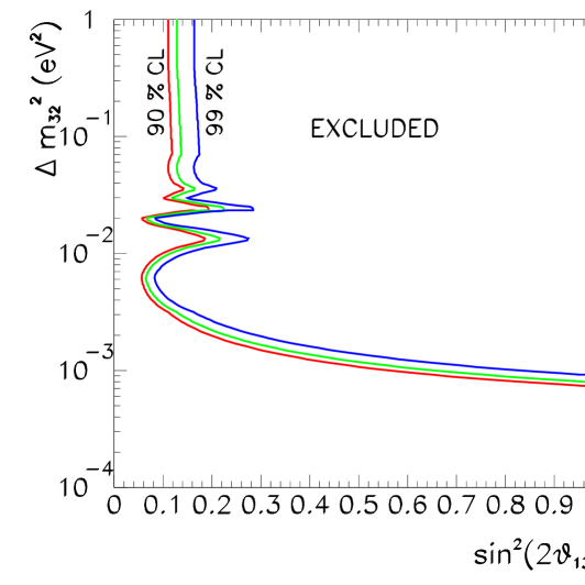
FIG. 1.: Excluded region in $\Delta{m}^{2}_{32}$ and $\sin^{2}(2\theta_{13})$ from the non observation of oscillations by the CHOOZ reactor experiment. The curves represent the 90, 95 and 99% CL excluded region defined with 2 d.o.f. for comparison with the CHOOZ published results.

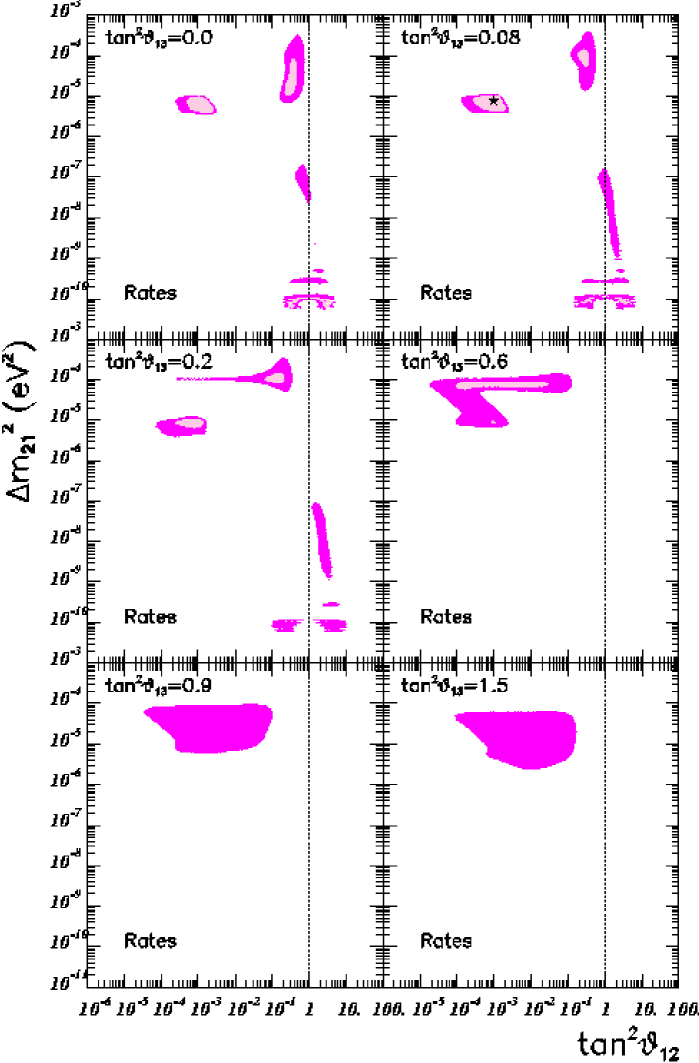
FIG. 2.: Allowed three–neutrino oscillation regions in $\Delta{m}^{2}_{21}$ and $\tan^{2}\theta_{12}$ from the measurements of the total event rates at Chlorine, Gallium, Kamiokande and Super–Kamiokande (1117-day data sample) experiments. The different panels represent the allowed regions at 99% (darker) and 90% CL (lighter) obtained as sections for fixed values of the mixing angle $\tan^{2}\theta_{13}$ of the three–dimensional volume defined by $\chi^{2}-\chi^{2}_{min}$=6.25 (90%), 11.36 (99%). The best–fit point is denoted as a star.

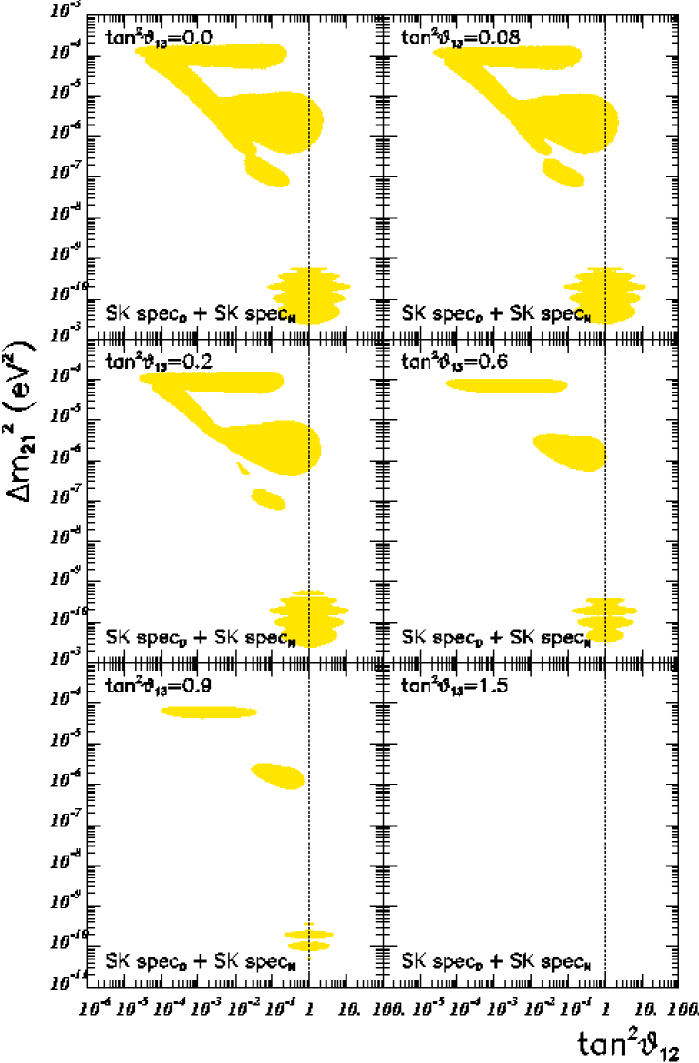
FIG. 3.: Excluded three–neutrino solar oscillation regions at 99% CL in $\Delta{m}^{2}_{21}$ and $\tan^{2}\theta_{12}$ from the measurement of the day–night spectra data by Super–Kamiokande (1117-day data sample).

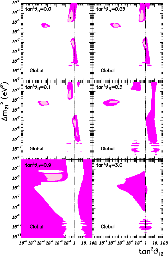
FIG. 4.: Allowed three–neutrino solar oscillation regions in $\Delta{m}^{2}_{21}$ and $\tan^{2}\theta_{12}$ from the global analysis of solar neutrino data. The best–fit point is denoted as a star.

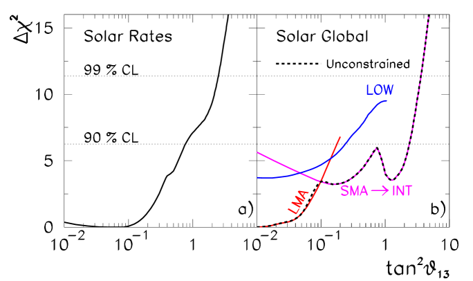
FIG. 5.: $\Delta\chi^{2}$ as a function of $\tan^{2}\theta_{13}$ from the three–neutrino analysis of the solar data. The left panel corresponds the analysis of total rates only and the right panel to the global analysis. The dotted horizontal lines correspond to the 90%, 99% CL limits.

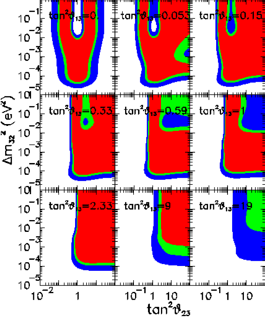
FIG. 6.: Allowed $(\tan^{2}\theta_{23},\Delta m^{2}_{32})$ regions for different $\tan^{2}\theta_{13}$ values, for the FINKS combination of atmospheric neutrino data. The regions refer to 90, 95 and 99% CL. The best–fit point in the three parameter space is denoted as a star.

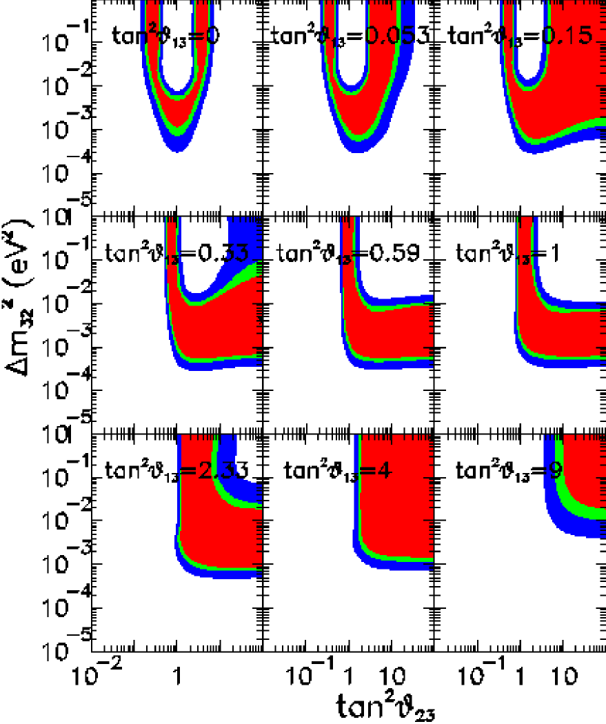
FIG. 7.: Allowed three–neutrino $(\tan^{2}\theta_{23},\Delta m^{2}_{32})$ regions for different $\tan^{2}\theta_{13}$ values, for the CONT–UNBIN combination of atmospheric neutrino data. The regions refer to 90, 95 and 99% CL. The best–fit point is denoted as a star.

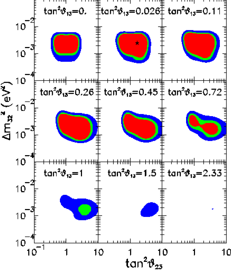
FIG. 8.: Allowed three–neutrino $(\tan^{2}\theta_{23},\Delta m^{2}_{32})$ regions for different $\tan^{2}\theta_{13}$ values, for the CONT–BIN combination of atmospheric neutrino events The regions refer to 90, 95 and 99% CL. The best–fit point is denoted as a star.

FIG. 9.: Zenith-angle distributions for the Super–Kamiokande $e$–like (left panels) and $\mu$–like (right-panels) events, both in the sub-GeV (upper panels) and multi-GeV (lower panels) energy range. The thick solid line is the expected distribution in the SM. The thin full line is the prediction for the overall best-fit point of ALL–ATM data $\tan^{2}\theta_{13}=0.025$, $\Delta m^{2}_{32}=3.3\times 10^{-3}$ eV² and $\tan^{2}\theta_{23}=1.6$. The dashed (dotted) histogram correspond to the distributions for $\Delta m^{2}_{32}=3.3\,(2.85)\times 10^{-3}$ eV², $\tan^{2}\theta_{23}=3.0\,(3.1)$ and $\tan^{2}\theta_{13}=0.33\,(0.54)$ which are allowed at 90 (99)% CL.

FIG. 10.: 90, 95 and 99% three–neutrino allowed regions in the $(\tan^{2}\theta_{23},\Delta m^{2}_{32})$ plane for different $\tan^{2}\theta_{13}$ values, for the combination of UP–$\mu$ events induced by atmospheric neutrinos from Super–Kamiokande (through–going and stopping) and MACRO (through–going only). The best–fit point is denoted as a star.

FIG. 11.: Zenith-angle distributions for upward-going muon events in Super–Kamiokande and MACRO. The thick solid line is the expected distribution in the SM. The thin full line is the prediction for the overall best-fit point of ALL–ATM data $\tan^{2}\theta_{13}=0.025$, $\Delta m^{2}_{32}=3.3\times 10^{-3}$ eV² and $\tan^{2}\theta_{23}=1.6$. The dashed (dotted) histogram correspond to the distributions for $\Delta m^{2}_{32}=3.3\,(2.85)\times 10^{-3}$ eV², $\tan^{2}\theta_{23}=3.0\,(3.1)$ and $\tan^{2}\theta_{13}=0.33\,(0.54)$ which are allowed at 90 (99)% CL.

FIG. 12.: Allowed $(\tan^{2}\theta_{23},\Delta m^{2}_{32})$ regions for different $\tan^{2}\theta_{13}$ values, for the combination of SK atmospheric neutrino events. The regions refer to 90, 95 and 99% CL. The best–fit point is denoted as a star.

FIG. 13.: 90, 95 and 99% CL three–neutrino allowed regions in $(\tan^{2}\theta_{23},~{}\Delta m^{2}_{32})$ for different $\tan^{2}\theta_{13}$ values, for the combination of ALL–ATM neutrino data. The best–fit point is denoted as a star.

FIG. 14.: Dependence of the $\Delta\chi^{2}$ function on $\tan^{2}\theta_{13}$ and on $\Delta m^{2}_{32}$ , for different combinations of atmospheric neutrino events. The dotted horizontal lines correspond to the 90%, 99% CL limits.

FIG. 15.: Dependence of the $\Delta\chi^{2}$ function on $\tan^{2}\theta_{13}$ and on $\Delta m^{2}_{32}$, for the combination ALL–ATM of atmospheric neutrino data. The dashed line includes also the data from CHOOZ. The dotted horizontal lines correspond to the 90%, 99% CL limits for 3 d.o.f.

FIG. 16.: Allowed $(\tan^{2}\theta_{23},~{}\tan^{2}\theta_{13})$ regions for different $\Delta m^{2}_{32}$ values, for the combination ALL–ATM of atmospheric neutrino data.

FIG. 17.: Same as Fig. 8, but including also the CHOOZ result. The best–fit point is denoted as a star.

FIG. 18.: Same as Fig. 13, but including also the CHOOZ result. The best–fit point is denoted as a star.

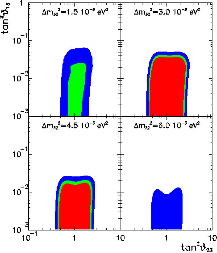
FIG. 19.: Same as Fig. 16, but including also the CHOOZ result.

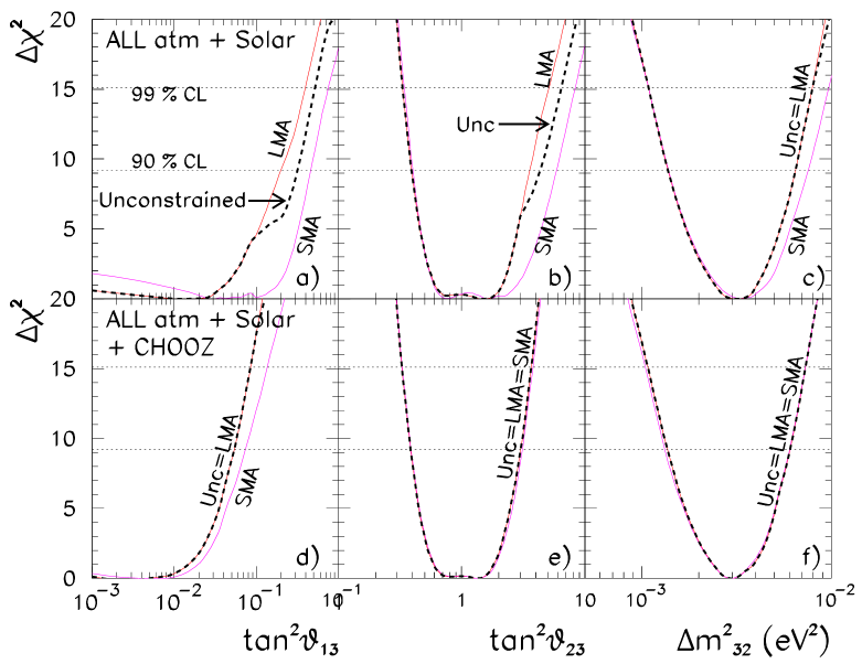
FIG. 20.: Dependence of $\Delta\chi^{2}$ on $\tan^{2}\theta_{13}$, $\tan^{2}\theta_{23}$ and on $\Delta m^{2}_{32}$ , for the analysis of atmospheric and solar neutrino events (upper panels) and atmospheric, solar and CHOOZ data (lower panels). The dotted horizontal lines correspond to the 90% and 99% CL limits for 5 d.o.f.

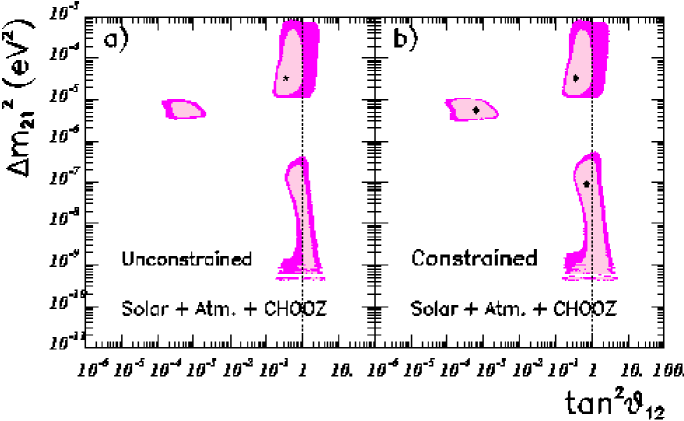
FIG. 21.: Allowed regions in $\Delta{m}^{2}_{21}$ and $\tan^{2}\theta_{12}$ from the global analysis of solar, atmospheric and reactor neutrino data. (a) Regions for the unconstrained analysis defined in terms of the increases of $\Delta\chi^{2}$ for 5 d.o.f. from the global best fit point denoted as a star. (b) Regions for the constrained analysis defined in terms of the increases of $\Delta\chi^{2}$ for 5 d.o.f. from the local best fit point denoted as a dot

.