hep-ph/0009343 VUTH 00-23 Transverse Momentum Dependence in Gluon Distribution and Fragmentation Functions

Abstract

We investigate the twist two gluon distribution functions for spin 1/2 hadrons, emphasizing intrinsic transverse momentum of the gluons. These functions are relevant in leading order in the inverse hard scale in scattering processes such as inclusive leptoproduction or Drell-Yan scattering, or more general in hard processes in which at least two hadrons are involved. They show up in azimuthal asymmetries. For future estimates of such observables, we discuss specific bounds on these functions.

I Introduction

Gluon distribution and fragmentation functions are fundamental quantities in the study of deep inelastic scattering processes. In fact, together with their quark and antiquark analogues, these process-independent quantities describe the soft parts of the scattering or, in other words, the deep structure of the hadrons. The partonic (distribution and fragmentation) functions cannot yet be calculated from first principles because we lack the non-perturbative treatment of the strong interactions. However, valuable information on these functions can be obtained via lattice calculations or theoretical models.

As soon as more than one hadron is involved in a hard scattering process, it is essential to take into account the transverse momentum of the partons. For instance, transverse momentum dependent quark distribution and fragmentation functions show up explicitly in several semi-inclusive cross sections, in particular in azimuthal asymmetries. In the calculation of QCD corrections for these cross sections, the inclusion of transverse momentum dependent gluon distributions and fragmentation functions will be necessary. This is our motivation to study in this paper the transverse momentum dependent gluon functions. We will follow the corresponding treatment for quarks developed by Mulders and Tangerman [1, 2], following earlier work by Ralston and Soper [3].

In a diagrammatic expansion of the hadronic tensor in powers of the strong coupling, one finds an infinite number of gluon correlators, which are essentially matrix elements of non-local products of gluons fields (and sometimes quark fields) between hadronic states. The simplest of these matrix elements are the ones that contain only two gluon fields. In the $A^{+}=0$ gauge, they completely define the twist two functions through the appropriate choice of Lorentz indices and projections. One has to make sure that the starting point is a gauge invariant object, which turns out to be a non-trivial matter.

More complicated correlators, namely with three gluon fields, must also be studied. Some of these correlators will precisely provide the link operator needed to define gauge invariant functions, and others will reduce to gluon-gluon and gluon-quark correlators using the QCD equations of motion. We will discard all correlators that contribute at order $1/Q^{2}$ or higher in the cross sections, $Q$ being the hard scale.

The paper is organized as follows. In the next section we start from the gauge invariant gluon-gluon correlation function and derive all twist two and three gluon distributions and we make an analysis of the link operator. We show that the link appears naturally when a certain class of diagrams is summed leading to a specific path. In section III we introduce a specific helicity basis for nucleons and give the spin representation of the twist two part of the gluon-gluon correlator, which can be used to derive the natural interpretation of the lower twist functions as gluon densities in the framework of the parton model. In section IV the formalism is extended to the gluon fragmentation functions, after which we discuss some bounds. We end up with some conclusions and suggestions for future investigations that can use the formalism developed in this paper.

II Gluon Correlation Functions

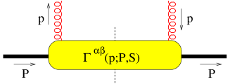
FIG. 1.: The gluon correlator

In order to connect gluons in a hard scattering process to hadrons appearing in the initial or final state, we will use (lightcone) correlation functions [4, 5, 6, 7]. Our starting point is the correlation function

$$S^{\mu\nu}(k;P,S;n)=\int{d^{4}\xi\over{(2\pi)}^{4}}\ e^{ik\cdot\xi}\langle P,S|A^{\mu}(0)A^{\nu}(\xi)|P,S\rangle,$$ (1)

diagrammatically represented in Fig. 1. The vectors $P$ and $S$ are respectively the momentum and the spin of the hadron, while $k$ stands for the momentum of the gluon. Additional dependence can come for instance from fixing the gauge using a vector $n$. A summation over color indices is understood. If, as done in this paper we use the notation $A_{\mu}(\xi)\equiv A^{a}_{\mu}(\xi)T^{a}$, where the $T^{a}$ are the generators of the $SU(3)$ color group, this summation is actually an appropriate tracing.

A corresponding gauge invariant object is the quantity

$$\Gamma^{\mu\nu;\rho\sigma}(k;P,S)=\int{d^{4}\xi\over(2\pi)^{4}}\ e^{ik\cdot\xi}\ \langle P,S|F^{\mu\nu}(0)\ {\cal U}(0,\xi)\ F^{\rho\sigma}(\xi)|P,S\rangle,$$ (2)

where $F_{\mu\nu}(\xi)\equiv F_{\mu\nu}^{a}(\xi)T^{a}$ is the field tensor, related to the potential by $F_{\mu\nu}=\partial_{\mu}A_{\nu}-\partial_{\nu}A_{\mu}-ig\left[A_{\mu},A_{\nu}\right]$. The link operator ${\cal U}$ will be studied in detail in one of the next sections.

A The Lorentz structure of the gluon correlator

The Lorentz structure of the gluon correlator is limited by constraints following from hermiticity and parity conservation. These are

$$\Gamma^{\rho\sigma;\mu\nu*}(k;P,S) = \Gamma^{\mu\nu;\rho\sigma}(k;P,S),$$ (3)

$$\Gamma^{\mu\nu;\rho\sigma}(k;P,S) = \Gamma_{\mu\nu;\rho\sigma}(\overline{k};\overline{P},-\overline{S}),$$ (4)

where $\overline{k}$ = $(k^{0},-k^{i})$. A possible parameterization of $\Gamma^{\mu\nu;\rho\sigma}$ compatible with these constraints is

$$\Gamma^{\mu\nu;\rho\sigma}(k;P,S) = X_{1}\epsilon^{\mu\nu\alpha\beta}\left.\epsilon^{\rho\sigma}\right._{\alpha\beta}+{X_{2}\over M^{2}}P^{\left[\mu\right.}g^{\left.\nu\right]\left[\rho\right.}P^{\left.\sigma\right]}+{X_{3}\over M^{2}}\ k^{\left[\mu\right.}g^{\left.\nu\right]\left[\rho\right.}k^{\left.\sigma\right]}$$ (16)

$$+{X_{4}+iX_{5}\over M^{2}}\ P^{\left[\mu\right.}g^{\left.\nu\right]\left[\rho\right.}k^{\left.\sigma\right]}+{X_{4}-iX_{5}\over M^{2}}\ k^{\left[\mu\right.}g^{\left.\nu\right]\left[\rho\right.}P^{\left.\sigma\right]}$$

$$+{X_{6}\over M^{4}}\ P^{\left[\mu\right.}k^{\left.\nu\right]}P^{\left[\rho\right.}k^{\left.\sigma\right]}-{2X_{7}\over M}\ \epsilon^{\mu\nu\rho\sigma}(k\cdot S)$$

$$+i{X_{8}\over M}\ \epsilon^{\mu\nu P\left[\sigma\right.}S^{\left.\rho\right]}+i{X_{9}\over M}\ \epsilon^{\mu\nu S\left[\sigma\right.}P^{\left.\rho\right]}$$

$$+i{X_{10}\over M}\ \epsilon^{\mu\nu k\left[\sigma\right.}S^{\left.\rho\right]}+i{X_{11}\over M}\ \epsilon^{\mu\nu S\left[\sigma\right.}k^{\left.\rho\right]}$$

$$+i{X_{12}\over M^{3}}\ \epsilon^{\mu\nu P\left[\sigma\right.}P^{\left.\rho\right]}(k\cdot S)+i{X_{13}\over M^{3}}\ \epsilon^{\mu\nu k\left[\sigma\right.}k^{\left.\rho\right]}(k\cdot S)$$

$$+i{X_{14}\over M^{3}}\ \epsilon^{\mu\nu P\left[\sigma\right.}k^{\left.\rho\right]}(k\cdot S)+i{X_{15}\over M^{3}}\ \epsilon^{\mu\nu k\left[\sigma\right.}P^{\left.\rho\right]}(k\cdot S)$$

$$+{X_{16}+iX_{17}\over M^{3}}\ \epsilon^{\mu\nu PS}\ k^{\left[\rho\right.}P^{\left.\sigma\right]}+{X_{16}-iX_{17}\over M^{3}}\ \epsilon^{\rho\sigma PS}\ k^{\left[\mu\right.}P^{\left.\nu\right]}$$

$$+{X_{18}+iX_{19}\over M^{3}}\ \epsilon^{\mu\nu kS}\ k^{\left[\rho\right.}P^{\left.\sigma\right]}+{X_{18}-iX_{19}\over M^{3}}\ \epsilon^{\rho\sigma kS}\ k^{\left[\mu\right.}P^{\left.\nu\right]}$$

$$+{X_{20}+iX_{21}\over M^{3}}\ \epsilon^{\mu\nu kP}\ P^{\left[\rho\right.}S^{\left.\sigma\right]}+{X_{20}-iX_{21}\over M^{3}}\ \epsilon^{\rho\sigma kP}\ P^{\left[\mu\right.}S^{\left.\nu\right]}$$

$$+{X_{22}+iX_{23}\over M^{3}}\ \epsilon^{\mu\nu kP}\ k^{\left[\rho\right.}S^{\left.\sigma\right]}+{X_{22}-iX_{23}\over M^{3}}\ \epsilon^{\rho\sigma kP}\ k^{\left[\mu\right.}S^{\left.\nu\right]}$$

$$+{X_{24}+iX_{25}\over M^{5}}\ \epsilon^{\mu\nu kP}\ k^{\left[\rho\right.}P^{\left.\sigma\right]}(k\cdot S)+{X_{24}-iX_{25}\over M^{5}}\ \epsilon^{\rho\sigma kP}\ k^{\left[\mu\right.}P^{\left.\nu\right]}(k\cdot S).$$

The amplitudes $X_{i}$ as well as the original correlator $\Gamma^{\mu\nu;\rho\sigma}(k;P,S)$ have dimensions $M^{-2}$. With the chosen parametrization, i.e. the appropriate introduction of factors 1 or $i$ for symmetric and antisymmetric tensors, hermiticity in Eq. (3) implies that one finds real amplitudes $X_{i}$. The parity constraint in Eq. (4) requires that even numbers of $\epsilon$-tensors are combined only with vectors $k$ and $P$, while odd numbers of $\epsilon$-tensors are combined with the axial vector $S$ besides vectors $k,P$. Since $S$ parametrizes the nucleon density matrix, it can only appear linearly.

Time reversal invariance, when applicable, imposes a third condition,

$$\Gamma_{\mu\nu;\rho\sigma}(\overline{k};\overline{P},\overline{S})={\Gamma^{\mu\nu;\rho\sigma}}^{*}(k;P,S),$$ (17)

which implies $X_{i}^{\ast}=-X_{i}$ for the amplitudes $X_{5}$, $X_{7}$, $X_{16}$, $X_{18}$, $X_{20}$, $X_{22}$ and $X_{24}$. For this reason, such amplitudes are called T-odd. They thus vanish when time-reversal can be used as a constraint.

B Twist expansion

Leading and non-leading contributions to the hadronic tensor are easier to identify if one uses a suitable parameterization of the hadron momentum and spin vectors in terms of two light-like directions, $n_{\scriptscriptstyle+}$ and $n_{\scriptscriptstyle-}$ (such that $n_{\scriptscriptstyle+}\cdot n_{\scriptscriptstyle-}=1$), and two transverse directions. They are chosen such that the hadrons have no transverse momentum, what means that $P$ can be written in terms of the light-like vectors. The momentum of the gluon and the spin vector of the hadron must include a transverse component:

$$P = P^{+}n_{\scriptscriptstyle+}+{M^{2}\over 2P^{+}}\ n_{\scriptscriptstyle-},$$ (18)

$$k = xP^{+}n_{\scriptscriptstyle+}+{k^{2}+{\mathchoice{{\hbox{\boldmath$\displaystyle k$}}}{{\hbox{\boldmath$\textstyle k$}}}{{\hbox{\boldmath$\scriptstyle k$}}}{{\hbox{\boldmath$\scriptscriptstyle k$}}}}_{\scriptscriptstyle T}^{2}\over 2xP^{+}}\ n_{\scriptscriptstyle-}+k_{\scriptscriptstyle T},$$ (19)

$$S = S_{\scriptscriptstyle L}{P^{+}\over M}\ n_{\scriptscriptstyle+}-S_{\scriptscriptstyle L}{M\over 2P^{+}}\ n_{\scriptscriptstyle-}+S_{\scriptscriptstyle T}.$$ (20)

The quantity $x$ represents the fraction of the light-cone momentum in the $+$ direction carried by the parton. The parameter $S_{\scriptscriptstyle L}$ and the two component vector ${\mathchoice{{\hbox{\boldmath$\displaystyle S$}}}{{\hbox{\boldmath$\textstyle S$}}}{{\hbox{\boldmath$\scriptstyle S$}}}{{\hbox{\boldmath$\scriptscriptstyle S$}}}}_{\scriptscriptstyle T}$ are such that $S_{\scriptscriptstyle L}^{2}+{\mathchoice{{\hbox{\boldmath$\displaystyle S$}}}{{\hbox{\boldmath$\textstyle S$}}}{{\hbox{\boldmath$\scriptstyle S$}}}{{\hbox{\boldmath$\scriptscriptstyle S$}}}}_{\scriptscriptstyle T}^{2}=1$. The quantity $S_{\scriptscriptstyle L}$ is referred to as the helicity. Having defined the $n_{\pm}$ vectors one has transverse tensors $g^{\mu\nu}_{\scriptscriptstyle T}$ and $\epsilon^{\mu\nu}_{\scriptscriptstyle T}$ defined as

$$g^{\mu\nu}_{\scriptscriptstyle T} \equiv g^{\mu\nu}-n_{\scriptscriptstyle+}^{\mu}n_{\scriptscriptstyle-}^{\nu}-n_{\scriptscriptstyle+}^{\nu}n_{\scriptscriptstyle-}^{\mu},$$ (21)

$$\epsilon^{\mu\nu}_{\scriptscriptstyle T} \equiv \epsilon^{n_{\scriptscriptstyle+}n_{\scriptscriptstyle-}\mu\nu}=\epsilon^{-+\mu\nu}.$$ (22)

The expansion in lightlike vectors shows its usefulness only when the correlation functions are used in a calculation of a hard scattering process in which a hard timelike or spacelike vector appears setting the hard scale. An example is the momentum transfer squared, $q^{2}=-Q^{2}$ in deep inelastic leptoproduction. For the soft part in the process, described with the correlation functions it implies that after all calculations are finished, the $P^{+}$ is of the same order of magnitude as the hard scattering scale $Q$. Simple power counting tells us that the most important contributions from $\Gamma^{\mu\nu;\rho\sigma}$ are the ones with the largest possible number of $+$ indices. Due to the antisymmetric character of the field tensor, these are obviously $\Gamma^{+i;+j}$ (referred to as twist two), followed by $\Gamma^{+i;+-}$ and $\Gamma^{ij;l+}$ (referred to as twist three), where $i,j,l,\ldots$ indicate transverse indices.

For deep inelastic scattering processes we always need the soft parts integrated over the momentum component $k^{-}$. Starting with the twist two part, we define

$$M\Gamma^{ij}(x,{\mathchoice{{\hbox{\boldmath$\displaystyle k$}}}{{\hbox{\boldmath$\textstyle k$}}}{{\hbox{\boldmath$\scriptstyle k$}}}{{\hbox{\boldmath$\scriptscriptstyle k$}}}}_{\scriptscriptstyle T})\equiv\int dk^{-}\ \Gamma^{+i;+j}(k;P,S)=\left.\int\frac{d\xi^{-}d^{2}\xi_{\scriptscriptstyle T}}{(2\pi)^{3}}\ e^{ik\cdot\xi}\,\langle P,S|F^{+i}(0)\,F^{+j}(\xi)|P,S\rangle\right|_{\xi^{+}=0}.$$ (23)

This quantity depends on the momentum fraction $x$ and the transverse momentum ${\mathchoice{{\hbox{\boldmath$\displaystyle k$}}}{{\hbox{\boldmath$\textstyle k$}}}{{\hbox{\boldmath$\scriptstyle k$}}}{{\hbox{\boldmath$\scriptscriptstyle k$}}}}_{\scriptscriptstyle T}$ besides the (suppressed) dependence on the target momentum and spin, and is conveniently expressed in terms of transverse tensors and vectors. Concerning the dependence on the hadron spin, we furthermore separate the unpolarized (O), longitudinally polarized (L) and transverse polarized (T) situations. This leads to

$$\Gamma_{O}^{ij}(x,{\mathchoice{{\hbox{\boldmath$\displaystyle k$}}}{{\hbox{\boldmath$\textstyle k$}}}{{\hbox{\boldmath$\scriptstyle k$}}}{{\hbox{\boldmath$\scriptscriptstyle k$}}}}_{\scriptscriptstyle T}) = {x\over 2}\ {P^{+}\over M}\left[-g^{ij}_{\scriptscriptstyle T}G(x,{\mathchoice{{\hbox{\boldmath$\displaystyle k$}}}{{\hbox{\boldmath$\textstyle k$}}}{{\hbox{\boldmath$\scriptstyle k$}}}{{\hbox{\boldmath$\scriptscriptstyle k$}}}}_{\scriptscriptstyle T}^{2})+\left({k_{\scriptscriptstyle T}^{i}k_{\scriptscriptstyle T}^{j}\over M^{2}}+g^{ij}_{\scriptscriptstyle T}{{\mathchoice{{\hbox{\boldmath$\displaystyle k$}}}{{\hbox{\boldmath$\textstyle k$}}}{{\hbox{\boldmath$\scriptstyle k$}}}{{\hbox{\boldmath$\scriptscriptstyle k$}}}}_{\scriptscriptstyle T}^{2}\over 2M^{2}}\right)H^{\perp}(x,{\mathchoice{{\hbox{\boldmath$\displaystyle k$}}}{{\hbox{\boldmath$\textstyle k$}}}{{\hbox{\boldmath$\scriptstyle k$}}}{{\hbox{\boldmath$\scriptscriptstyle k$}}}}_{\scriptscriptstyle T}^{2})\right],$$ (24)

$$\Gamma_{L}^{ij}(x,{\mathchoice{{\hbox{\boldmath$\displaystyle k$}}}{{\hbox{\boldmath$\textstyle k$}}}{{\hbox{\boldmath$\scriptstyle k$}}}{{\hbox{\boldmath$\scriptscriptstyle k$}}}}_{\scriptscriptstyle T}) = {x\over 2}\ {P^{+}\over M}\left[-i\epsilon^{ij}_{\scriptscriptstyle T}S_{\scriptscriptstyle L}\ \Delta G_{L}(x,{\mathchoice{{\hbox{\boldmath$\displaystyle k$}}}{{\hbox{\boldmath$\textstyle k$}}}{{\hbox{\boldmath$\scriptstyle k$}}}{{\hbox{\boldmath$\scriptscriptstyle k$}}}}_{\scriptscriptstyle T}^{2})+{\epsilon_{\scriptscriptstyle T}^{k_{\scriptscriptstyle T}\left\{i\right.}k_{\scriptscriptstyle T}^{\left.j\right\}}\over 2M^{2}}\ S_{\scriptscriptstyle L}\ \Delta H_{L}^{\perp}(x,{\mathchoice{{\hbox{\boldmath$\displaystyle k$}}}{{\hbox{\boldmath$\textstyle k$}}}{{\hbox{\boldmath$\scriptstyle k$}}}{{\hbox{\boldmath$\scriptscriptstyle k$}}}}_{\scriptscriptstyle T}^{2})\right],$$ (25)

$$\Gamma_{T}^{ij}(x,{\mathchoice{{\hbox{\boldmath$\displaystyle k$}}}{{\hbox{\boldmath$\textstyle k$}}}{{\hbox{\boldmath$\scriptstyle k$}}}{{\hbox{\boldmath$\scriptscriptstyle k$}}}}_{\scriptscriptstyle T}) = {x\over 2}\ {P^{+}\over M}\Biggl{[}-g^{ij}_{\scriptscriptstyle T}\ {\epsilon_{\scriptscriptstyle T}^{k_{\scriptscriptstyle T}S_{\scriptscriptstyle T}}\over M}\ G_{T}(x,{\mathchoice{{\hbox{\boldmath$\displaystyle k$}}}{{\hbox{\boldmath$\textstyle k$}}}{{\hbox{\boldmath$\scriptstyle k$}}}{{\hbox{\boldmath$\scriptscriptstyle k$}}}}_{\scriptscriptstyle T}^{2})-i\epsilon^{ij}_{\scriptscriptstyle T}\ {{\mathchoice{{\hbox{\boldmath$\displaystyle k$}}}{{\hbox{\boldmath$\textstyle k$}}}{{\hbox{\boldmath$\scriptstyle k$}}}{{\hbox{\boldmath$\scriptscriptstyle k$}}}}_{\scriptscriptstyle T}\cdot{\mathchoice{{\hbox{\boldmath$\displaystyle S$}}}{{\hbox{\boldmath$\textstyle S$}}}{{\hbox{\boldmath$\scriptstyle S$}}}{{\hbox{\boldmath$\scriptscriptstyle S$}}}}_{\scriptscriptstyle T}\over M}\ \Delta G_{T}(x,{\mathchoice{{\hbox{\boldmath$\displaystyle k$}}}{{\hbox{\boldmath$\textstyle k$}}}{{\hbox{\boldmath$\scriptstyle k$}}}{{\hbox{\boldmath$\scriptscriptstyle k$}}}}_{\scriptscriptstyle T}^{2})$$ (28)

$$\qquad\quad+{\epsilon_{\scriptscriptstyle T}^{k_{\scriptscriptstyle T}\{i}k_{\scriptscriptstyle T}^{j\}}\over 2M^{2}}{{\mathchoice{{\hbox{\boldmath$\displaystyle k$}}}{{\hbox{\boldmath$\textstyle k$}}}{{\hbox{\boldmath$\scriptstyle k$}}}{{\hbox{\boldmath$\scriptscriptstyle k$}}}}_{\scriptscriptstyle T}\cdot{\mathchoice{{\hbox{\boldmath$\displaystyle S$}}}{{\hbox{\boldmath$\textstyle S$}}}{{\hbox{\boldmath$\scriptstyle S$}}}{{\hbox{\boldmath$\scriptscriptstyle S$}}}}_{\scriptscriptstyle T}\over M}\ \Delta H_{T}^{\perp}(x,{\mathchoice{{\hbox{\boldmath$\displaystyle k$}}}{{\hbox{\boldmath$\textstyle k$}}}{{\hbox{\boldmath$\scriptstyle k$}}}{{\hbox{\boldmath$\scriptscriptstyle k$}}}}_{\scriptscriptstyle T}^{2})$$

$$\qquad\quad+{\epsilon_{\scriptscriptstyle T}^{k_{\scriptscriptstyle T}\left\{i\right.}S_{\scriptscriptstyle T}^{\left.j\right\}}+\epsilon_{\scriptscriptstyle T}^{S_{\scriptscriptstyle T}\left\{i\right.}k_{\scriptscriptstyle T}^{\left.j\right\}}\over 4M}\,\left[\Delta H_{T}(x,{\mathchoice{{\hbox{\boldmath$\displaystyle k$}}}{{\hbox{\boldmath$\textstyle k$}}}{{\hbox{\boldmath$\scriptstyle k$}}}{{\hbox{\boldmath$\scriptscriptstyle k$}}}}_{\scriptscriptstyle T}^{2})-\frac{{\mathchoice{{\hbox{\boldmath$\displaystyle k$}}}{{\hbox{\boldmath$\textstyle k$}}}{{\hbox{\boldmath$\scriptstyle k$}}}{{\hbox{\boldmath$\scriptscriptstyle k$}}}}_{\scriptscriptstyle T}^{2}}{2M^{2}}\,\Delta H_{T}^{\perp}(x,{\mathchoice{{\hbox{\boldmath$\displaystyle k$}}}{{\hbox{\boldmath$\textstyle k$}}}{{\hbox{\boldmath$\scriptstyle k$}}}{{\hbox{\boldmath$\scriptscriptstyle k$}}}}_{\scriptscriptstyle T}^{2})\right]\Biggr{]},$$

where the expressions of the functions in terms of the amplitudes $X_{i}$ can be found in the appendix. The factors in this parametrization are chosen in order that $G$ can be interpreted as the gluon momentum density [5], which will become clear when we discuss sum rules at the end of this section and in the next section. Actually also the use of the combination $\Delta H_{T}^{\prime}=\Delta H_{T}-\Delta H_{T}^{\perp(1)}$, where $\Delta H_{T}^{\perp(n)}\equiv({\mathchoice{{\hbox{\boldmath$\displaystyle k$}}}{{\hbox{\boldmath$\textstyle k$}}}{{\hbox{\boldmath$\scriptstyle k$}}}{{\hbox{\boldmath$\scriptscriptstyle k$}}}}_{\scriptscriptstyle T}^{2}/2M^{2})^{n}\Delta H_{T}^{\perp}$ (with similar definitions for other functions), is done because it is nicer for interpreting the functions.

When we use the soft parts in calculations up to ${\cal O}(1/Q)$ we need $\Gamma^{+i;+-}$ and $\Gamma^{ij;l+}$, again integrated over $dk^{-}$, which we refer to as twist three contributions,

$$M\Gamma^{i-}(x,{\mathchoice{{\hbox{\boldmath$\displaystyle k$}}}{{\hbox{\boldmath$\textstyle k$}}}{{\hbox{\boldmath$\scriptstyle k$}}}{{\hbox{\boldmath$\scriptscriptstyle k$}}}}_{\scriptscriptstyle T}) \equiv \int dk^{-}\ \Gamma^{+i;+-}(k;P,S),$$ (29)

$$M\Gamma^{ij,l}(x,{\mathchoice{{\hbox{\boldmath$\displaystyle k$}}}{{\hbox{\boldmath$\textstyle k$}}}{{\hbox{\boldmath$\scriptstyle k$}}}{{\hbox{\boldmath$\scriptscriptstyle k$}}}}_{\scriptscriptstyle T}) \equiv \int dk^{-}\ \Gamma^{ij;l+}(k;P,S).$$ (30)

They are again parametrized in terms of a number of functions. We obtain for the various hadron polarizations,

$$\Gamma_{O}^{i-}(x,{\mathchoice{{\hbox{\boldmath$\displaystyle k$}}}{{\hbox{\boldmath$\textstyle k$}}}{{\hbox{\boldmath$\scriptstyle k$}}}{{\hbox{\boldmath$\scriptscriptstyle k$}}}}_{\scriptscriptstyle T}) = {x\over 2}{k_{\scriptscriptstyle T}^{i}\over M}\ G_{3}^{\perp}(x,{\mathchoice{{\hbox{\boldmath$\displaystyle k$}}}{{\hbox{\boldmath$\textstyle k$}}}{{\hbox{\boldmath$\scriptstyle k$}}}{{\hbox{\boldmath$\scriptscriptstyle k$}}}}_{\scriptscriptstyle T}^{2}),$$ (31)

$$\Gamma_{L}^{i-}(x,{\mathchoice{{\hbox{\boldmath$\displaystyle k$}}}{{\hbox{\boldmath$\textstyle k$}}}{{\hbox{\boldmath$\scriptstyle k$}}}{{\hbox{\boldmath$\scriptscriptstyle k$}}}}_{\scriptscriptstyle T}) = {x\over 2}iS_{\scriptscriptstyle L}\ {\epsilon_{\scriptscriptstyle T}^{k_{\scriptscriptstyle T}i}\over M}\Delta G_{3L}^{\perp}(x,{\mathchoice{{\hbox{\boldmath$\displaystyle k$}}}{{\hbox{\boldmath$\textstyle k$}}}{{\hbox{\boldmath$\scriptstyle k$}}}{{\hbox{\boldmath$\scriptscriptstyle k$}}}}_{\scriptscriptstyle T}^{2}),$$ (32)

$$\Gamma_{T}^{i-}(x,{\mathchoice{{\hbox{\boldmath$\displaystyle k$}}}{{\hbox{\boldmath$\textstyle k$}}}{{\hbox{\boldmath$\scriptstyle k$}}}{{\hbox{\boldmath$\scriptscriptstyle k$}}}}_{\scriptscriptstyle T}) = {x\over 2}\left[i\epsilon_{\scriptscriptstyle T}^{S_{\scriptscriptstyle T}i}\ \Delta G_{3T}^{\prime}(x,{\mathchoice{{\hbox{\boldmath$\displaystyle k$}}}{{\hbox{\boldmath$\textstyle k$}}}{{\hbox{\boldmath$\scriptstyle k$}}}{{\hbox{\boldmath$\scriptscriptstyle k$}}}}_{\scriptscriptstyle T}^{2})+i{\epsilon_{\scriptscriptstyle T}^{k_{\scriptscriptstyle T}i}\over M}\ {{\mathchoice{{\hbox{\boldmath$\displaystyle k$}}}{{\hbox{\boldmath$\textstyle k$}}}{{\hbox{\boldmath$\scriptstyle k$}}}{{\hbox{\boldmath$\scriptscriptstyle k$}}}}_{\scriptscriptstyle T}\cdot{\mathchoice{{\hbox{\boldmath$\displaystyle S$}}}{{\hbox{\boldmath$\textstyle S$}}}{{\hbox{\boldmath$\scriptstyle S$}}}{{\hbox{\boldmath$\scriptscriptstyle S$}}}}_{\scriptscriptstyle T}\over M}\ \Delta G_{3T}^{\perp}(x,{\mathchoice{{\hbox{\boldmath$\displaystyle k$}}}{{\hbox{\boldmath$\textstyle k$}}}{{\hbox{\boldmath$\scriptstyle k$}}}{{\hbox{\boldmath$\scriptscriptstyle k$}}}}_{\scriptscriptstyle T}^{2})\right]$$ (33)

$$= {x\over 2}\left[i\epsilon_{\scriptscriptstyle T}^{S_{\scriptscriptstyle T}i}\ \Delta G_{3T}(x,{\mathchoice{{\hbox{\boldmath$\displaystyle k$}}}{{\hbox{\boldmath$\textstyle k$}}}{{\hbox{\boldmath$\scriptstyle k$}}}{{\hbox{\boldmath$\scriptscriptstyle k$}}}}_{\scriptscriptstyle T}^{2})+i\epsilon_{\scriptscriptstyle T}^{i\alpha}S_{\scriptscriptstyle T}^{\beta}\left({k_{{\scriptscriptstyle T}\alpha}k_{{\scriptscriptstyle T}\beta}\over M^{2}}+g_{T\alpha\beta}{{\mathchoice{{\hbox{\boldmath$\displaystyle k$}}}{{\hbox{\boldmath$\textstyle k$}}}{{\hbox{\boldmath$\scriptstyle k$}}}{{\hbox{\boldmath$\scriptscriptstyle k$}}}}_{\scriptscriptstyle T}^{2}\over 2M^{2}}\right)\Delta G_{3T}^{\perp}(x,{\mathchoice{{\hbox{\boldmath$\displaystyle k$}}}{{\hbox{\boldmath$\textstyle k$}}}{{\hbox{\boldmath$\scriptstyle k$}}}{{\hbox{\boldmath$\scriptscriptstyle k$}}}}_{\scriptscriptstyle T}^{2})\right],$$ (34)

and

$$\Gamma^{ij;l}_{O}(x,{\mathchoice{{\hbox{\boldmath$\displaystyle k$}}}{{\hbox{\boldmath$\textstyle k$}}}{{\hbox{\boldmath$\scriptstyle k$}}}{{\hbox{\boldmath$\scriptscriptstyle k$}}}}_{\scriptscriptstyle T}) = \ {x\over 2}\ {-g_{\scriptscriptstyle T}^{l\left[i\right.}k_{\scriptscriptstyle T}^{\left.j\right]}\over M}\ H_{3}^{\perp}(x,{\mathchoice{{\hbox{\boldmath$\displaystyle k$}}}{{\hbox{\boldmath$\textstyle k$}}}{{\hbox{\boldmath$\scriptstyle k$}}}{{\hbox{\boldmath$\scriptscriptstyle k$}}}}_{\scriptscriptstyle T}^{2}),$$ (35)

$$\Gamma^{ij;l}_{L}(x,{\mathchoice{{\hbox{\boldmath$\displaystyle k$}}}{{\hbox{\boldmath$\textstyle k$}}}{{\hbox{\boldmath$\scriptstyle k$}}}{{\hbox{\boldmath$\scriptscriptstyle k$}}}}_{\scriptscriptstyle T}) = {x\over 2}\ iS_{\scriptscriptstyle L}\epsilon^{ij}_{\scriptscriptstyle T}\ {k_{\scriptscriptstyle T}^{l}\over M}\ \Delta H_{3L}^{\perp}(x,{\mathchoice{{\hbox{\boldmath$\displaystyle k$}}}{{\hbox{\boldmath$\textstyle k$}}}{{\hbox{\boldmath$\scriptstyle k$}}}{{\hbox{\boldmath$\scriptscriptstyle k$}}}}_{\scriptscriptstyle T}^{2}),$$ (36)

$$\Gamma^{ij;l}_{T}(x,{\mathchoice{{\hbox{\boldmath$\displaystyle k$}}}{{\hbox{\boldmath$\textstyle k$}}}{{\hbox{\boldmath$\scriptstyle k$}}}{{\hbox{\boldmath$\scriptscriptstyle k$}}}}_{\scriptscriptstyle T}) = {x\over 2}\left[i\epsilon^{ij}_{\scriptscriptstyle T}S_{\scriptscriptstyle T}^{l}\ \Delta H_{3T}^{\prime}(x,{\mathchoice{{\hbox{\boldmath$\displaystyle k$}}}{{\hbox{\boldmath$\textstyle k$}}}{{\hbox{\boldmath$\scriptstyle k$}}}{{\hbox{\boldmath$\scriptscriptstyle k$}}}}_{\scriptscriptstyle T}^{2})+i\epsilon^{ij}_{\scriptscriptstyle T}\ {k_{\scriptscriptstyle T}^{l}\over M}\ {{\mathchoice{{\hbox{\boldmath$\displaystyle k$}}}{{\hbox{\boldmath$\textstyle k$}}}{{\hbox{\boldmath$\scriptstyle k$}}}{{\hbox{\boldmath$\scriptscriptstyle k$}}}}_{\scriptscriptstyle T}\cdot{\mathchoice{{\hbox{\boldmath$\displaystyle S$}}}{{\hbox{\boldmath$\textstyle S$}}}{{\hbox{\boldmath$\scriptstyle S$}}}{{\hbox{\boldmath$\scriptscriptstyle S$}}}}_{\scriptscriptstyle T}\over M}\ \Delta H_{3T}^{\perp}(x,{\mathchoice{{\hbox{\boldmath$\displaystyle k$}}}{{\hbox{\boldmath$\textstyle k$}}}{{\hbox{\boldmath$\scriptstyle k$}}}{{\hbox{\boldmath$\scriptscriptstyle k$}}}}_{\scriptscriptstyle T}^{2})\right]$$ (37)

$$= {x\over 2}\left[i\epsilon^{ij}_{\scriptscriptstyle T}S_{\scriptscriptstyle T}^{l}\ \Delta H_{3T}(x,{\mathchoice{{\hbox{\boldmath$\displaystyle k$}}}{{\hbox{\boldmath$\textstyle k$}}}{{\hbox{\boldmath$\scriptstyle k$}}}{{\hbox{\boldmath$\scriptscriptstyle k$}}}}_{\scriptscriptstyle T}^{2})-i\epsilon^{ij}_{\scriptscriptstyle T}\ S_{T\alpha}\left({k_{\scriptscriptstyle T}^{\alpha}k_{\scriptscriptstyle T}^{l}\over M^{2}}+g_{\scriptscriptstyle T}^{\alpha l}{{\mathchoice{{\hbox{\boldmath$\displaystyle k$}}}{{\hbox{\boldmath$\textstyle k$}}}{{\hbox{\boldmath$\scriptstyle k$}}}{{\hbox{\boldmath$\scriptscriptstyle k$}}}}_{\scriptscriptstyle T}^{2}\over 2M^{2}}\right)\ \Delta H_{3T}^{\perp}(x,{\mathchoice{{\hbox{\boldmath$\displaystyle k$}}}{{\hbox{\boldmath$\textstyle k$}}}{{\hbox{\boldmath$\scriptstyle k$}}}{{\hbox{\boldmath$\scriptscriptstyle k$}}}}_{\scriptscriptstyle T}^{2})\right]$$ (38)

Again the functions expressed in terms of the amplitudes are given in the appendix. While the functions for twist two are real functions, those for twist three are arranged in terms of complex functions in such a way that the T-even functions correspond to the real parts and the T-odd functions correspond to the imaginary parts. For twist two, the functions $G_{T}$, $\Delta H_{L}^{\perp}$, $\Delta H_{T}^{\perp}$, and $\Delta H_{T}$ are T-odd.

Let us make a short remark on the names of the functions, which follow for the indices in part the notations of quark distributions as introduced in [8] (and extended in [1, 2]). The distributions are represented by $G$, $H$, $\Delta G$ or $\Delta H$. The names $G$ and $\Delta G$ are reserved for functions that do not involve uncontracted momentum indices. These do not flip the gluon helicity, and represent unpolarized ($G$) and polarized ($\Delta G$) gluons, respectively. The functions $H$ and $\Delta H$ flip gluon helicity in unpolarized or polarized targets respectively, as we will discuss in detail below. We distinguish between the longitudinally polarized spin 1/2 target being multiplied by $S_{\scriptscriptstyle L}$, which acquire a subscript $L$ and those appearing in a transversely polarized spin 1/2 target being multiplied by the transverse spin of the hadron, which acquire a subscript $T$. If there is an uncontracted component of the transverse momentum of the gluon multiplying the function or if needed to avoid double names, we add a superscript $\perp$. Finally, twist three functions are given an additional subscript ‘3’.

In the next step we perform the integration over the transverse momentum of the gluon to arrive at the distribution functions which depend only on $x$ and are important in deep inelastic inclusive measurements. We define

$$\Gamma^{ij}(x)\equiv\int d^{2}{\mathchoice{{\hbox{\boldmath$\displaystyle k$}}}{{\hbox{\boldmath$\textstyle k$}}}{{\hbox{\boldmath$\scriptstyle k$}}}{{\hbox{\boldmath$\scriptscriptstyle k$}}}}_{\scriptscriptstyle T}\ \Gamma^{ij}(x,{\mathchoice{{\hbox{\boldmath$\displaystyle k$}}}{{\hbox{\boldmath$\textstyle k$}}}{{\hbox{\boldmath$\scriptstyle k$}}}{{\hbox{\boldmath$\scriptscriptstyle k$}}}}_{\scriptscriptstyle T})=\left.\int\frac{d\xi^{-}}{2\pi}\ e^{ik\cdot\xi}\,\langle P,S|F^{+i}(0)\,F^{+j}(\xi)|P,S\rangle\right|_{\xi^{+}=\xi_{\scriptscriptstyle T}=0},$$ (39)

and similarly for $\Gamma^{i-}(x)$ and $\Gamma^{ij;l}(x)$.

We find (combining the polarizations)

$$\Gamma^{ij}(x) = {x\over 2}\ {P^{+}\over M}\left[-g^{ij}_{\scriptscriptstyle T}G(x)-S_{\scriptscriptstyle L}i\epsilon^{ij}_{\scriptscriptstyle T}\ \Delta G(x)\right],$$ (40)

$$\Gamma^{i-}(x) = {x\over 2}\ i\epsilon_{\scriptscriptstyle T}^{S_{\scriptscriptstyle T}i}\ \Delta G_{3T}(x),$$ (41)

$$\Gamma^{ij,l}(x) = {x\over 2}\ i\epsilon_{\scriptscriptstyle T}^{ij}S_{\scriptscriptstyle T}^{l}\ \Delta H_{3T}(x).$$ (42)

where $G(x)=\int d^{2}{\mathchoice{{\hbox{\boldmath$\displaystyle k$}}}{{\hbox{\boldmath$\textstyle k$}}}{{\hbox{\boldmath$\scriptstyle k$}}}{{\hbox{\boldmath$\scriptscriptstyle k$}}}}_{\scriptscriptstyle T}\ G(x,{\mathchoice{{\hbox{\boldmath$\displaystyle k$}}}{{\hbox{\boldmath$\textstyle k$}}}{{\hbox{\boldmath$\scriptstyle k$}}}{{\hbox{\boldmath$\scriptscriptstyle k$}}}}_{\scriptscriptstyle T}^{2})$ and similarly for $\Delta G_{3T}$ and $\Delta H_{3T}$, while $\Delta G(x)=\int d^{2}{\mathchoice{{\hbox{\boldmath$\displaystyle k$}}}{{\hbox{\boldmath$\textstyle k$}}}{{\hbox{\boldmath$\scriptstyle k$}}}{{\hbox{\boldmath$\scriptscriptstyle k$}}}}_{\scriptscriptstyle T}\Delta G_{L}(x,{\mathchoice{{\hbox{\boldmath$\displaystyle k$}}}{{\hbox{\boldmath$\textstyle k$}}}{{\hbox{\boldmath$\scriptstyle k$}}}{{\hbox{\boldmath$\scriptscriptstyle k$}}}}_{\scriptscriptstyle T}^{2})$. The functions $\Delta G_{3T}$ and $\Delta H_{3T}$ are in essence the functions $H_{1}$ and $H_{2}$ of Ref. [6].

C Sum rules

Local hadronic matrix elements are obtained from the gluon correlation functions after integration over $dk^{+}$, e.g.

$$M^{2}\Gamma^{ij}\equiv M\int dk^{+}\ \Gamma^{ij}(x)=\langle P,S|F^{+\mu}(0)F^{+\nu}(0)|P,S\rangle.$$ (43)

The trace of this quantity is precisely the gluon part of the energy momentum tensor. Using the parametrization of $\Gamma^{ij}(x)$ in terms of the gluon distribution $G(x)$ one finds

$$M^{2}\Gamma^{ii}=2(P^{+})^{2}\int_{0}^{1}dx\ xG(x)=\langle P,S|\theta^{++}|P,S\rangle.$$ (44)

To derive this last relation we used the fact that the integral over $dx$ has a support between $-1$ and $+1$ and the symmetry relation $G(-x)=-G(x)$, which follows from the commutation relations for gluonic fields. The number

$$\epsilon_{g}=\int_{0}^{1}dx\ xG(x)$$ (45)

thus is identified with the fraction of light-cone momentum carried by the gluons, $0\leq\epsilon_{g}\leq 1$.

D Gauge Invariance

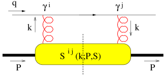
(a)

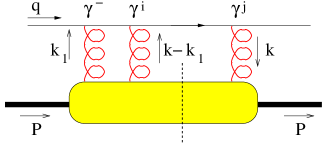
(b)

FIG. 2.: Some contributions to the fictitious highly virtual fermion-nucleon cross section

Of course the object appearing in the diagrammatic expansion, $S^{ij}(k;P,S)$, is not gauge invariant. We solved half of the problem by starting with $\Gamma^{\mu\nu;\rho\sigma}$. In particular, in the $A^{+}=0$ gauge one has $F^{+i}=\partial^{+}A_{T}^{i}$ and thus

$$\Gamma^{+i;+j}(k;P,S)=-(k^{+})^{2}\ S^{ij}(k;P,S).$$ (46)

In a general gauge, however, one also needs to consider matrix elements of the form $\langle A^{i}A^{+}A^{j}\rangle$, $\langle A^{i}A^{+}A^{+}A^{j}\rangle$, etc. Two simple leading contributions are shown in a fictitious highly virtual fermion-nucleon scattering process in Fig. 2. These will contribute at the same order in an expansion in the inverse hard scale. They will assure that in a general gauge one also finds other terms such as $[A^{+},A^{i}]$ terms in $F^{+i}$, and more importantly a gauge link operator. To be precise in a fictitious calculation as in Fig. 2 one finds that the field $A_{T}^{i}(\xi)$ appearing in the correlator in Eq. 1 is to be replaced by

$$A_{T}^{i}(\xi)=\int_{\infty}^{\xi^{-}}d\eta^{-}\ {\cal U}(\infty,\eta)\,F^{+i}(\eta),$$ (47)

where $\eta^{+}=\xi^{+}=0$, and $\eta_{\scriptscriptstyle T}$ = $\xi_{\scriptscriptstyle T}$ and

$${\cal U}(\infty,\xi)={\cal P}\ \exp\left(-ig\int_{\infty}^{\xi}ds^{\mu}A_{\mu}(s)\right),$$ (48)

where the path runs along the minus direction from the point $\xi^{-}=\infty$ to $\xi^{-}$ with $\xi^{+}$ = 0 and $\xi_{\scriptscriptstyle T}$ fixed, analogous to the path for quark correlators [9]. In the $k_{\scriptscriptstyle T}$ integrated correlators both links run along $\xi_{\scriptscriptstyle T}$ = 0 and a straight link between the lightlike separated points in the $\langle F^{+i}(0)\,F^{+j}(\xi)\rangle$ correlator in Eq. 39 remains. For the non-integrated correlator in Eq. 23 the links do not close, but with the physical assumption that hadronic matrix elements of the type $\langle A_{T}^{i}(0)A_{T}^{j}(\eta^{-}=\infty)A_{T}^{j}(\xi^{-})\rangle$ vanish this does not pose a problem. Furthermore when considering weighted $k_{\scriptscriptstyle T}$-integrated cross sections as was for instance done for quark field correlators in Ref. [10], one anyway reduces the matrix elements to lightlike separations.

We note that in different processes, e.g. lepton-hadron scattering or Drell-Yan scattering the paths will run from different points, that is $\xi^{-}$ = $\infty$ and $-\infty$, respectively. In $A^{+}=0$ gauge, the difference, however, is precisely $A^{i}_{\scriptscriptstyle T}(\xi^{-}=\infty)+A_{\scriptscriptstyle T}^{i}(\xi^{-}=-\infty)$, a quantity remaining to be fixed to fully fix the lightcone gauge [11, 12].

III The Twist Two Functions as densities

The fact that we in the gauge $A^{+}=0$ are left with $S^{ij}$, a matrix element bilinear in the gluonic fields, suggests that it might be possible to find a probabilistic interpretation for some distribution functions. This has been discussed in detail in several papers, expanding the transverse gluon fields in modes. We follow here a slightly different route that allows us to draw conclusions on the newly introduced leading twist transverse momentum dependent functions of the previous section.

The basic idea is the observation that $M^{ij}\equiv(2M/xP^{+})\Gamma^{ij}$ is a two by two matrix in the two transverse polarizations that for any diagonal element is a (positive-definite) density. Generalizing also to a matrix in the hadron spin space, one has

$$\Gamma^{ij}_{\Lambda\Lambda^{\prime}}(x) = \left.\int\frac{d\xi^{-}}{2\pi}\ e^{ik\cdot\xi}\langle P,\Lambda|F^{+i}(0)\,F^{+j}(\xi)|P,\Lambda^{\prime}\rangle\right|_{\xi^{+}=\xi_{\scriptscriptstyle T}=0}$$ (49)

$$= \sum_{n}\langle P_{n}|F^{+i}(0)|P,\Lambda\rangle^{*}\langle P_{n}|F^{+j}(0)|P,\Lambda^{\prime}\rangle\,\delta\left(P_{n}^{+}-(1-x)P^{+}\right).$$ (50)

In principle it does not matter for our considerations if we use the matrix for (real) linear polarizations or for the circular polarizations of the gluons. For interpretational purposes, the latter however is more common. Using the circular polarizations

$$|\pm\rangle=\mp\frac{1}{\sqrt{2}}\left(|x\rangle\pm i\,|y\rangle\right),$$ (51)

we obtain the matrix elements

$$M^{++} = {1\over 2}(M^{11}+M^{22})-{\cal I}m\,M^{12},$$ (52)

$$M^{+-} = -{1\over 2}(M^{11}-M^{22})+i\,{\cal R}e\,M^{12},$$ (53)

$$M^{-+} = -{1\over 2}(M^{11}-M^{22})-i\,{\cal R}e\,M^{12},$$ (54)

$$M^{--} = {1\over 2}(M^{11}+M^{22})+{\cal I}m\,M^{12}.$$ (55)

Explicitly we find from the parameterization in Eqs 24 - 28 the matrix elements (in gluon polarization space),

$$M^{++} = G+S_{\scriptscriptstyle L}\ \Delta G_{L}-S_{T}^{1}\ {|{\mathchoice{{\hbox{\boldmath$\displaystyle k$}}}{{\hbox{\boldmath$\textstyle k$}}}{{\hbox{\boldmath$\scriptstyle k$}}}{{\hbox{\boldmath$\scriptscriptstyle k$}}}}_{\scriptscriptstyle T}|\over M}(\sin\phi\ G_{T}-\cos\phi\ \Delta G_{T})+S_{T}^{2}\ {|{\mathchoice{{\hbox{\boldmath$\displaystyle k$}}}{{\hbox{\boldmath$\textstyle k$}}}{{\hbox{\boldmath$\scriptstyle k$}}}{{\hbox{\boldmath$\scriptscriptstyle k$}}}}_{\scriptscriptstyle T}|\over M}(\cos\phi\ G_{T}+\sin\phi\ \Delta G_{T}),$$ (56)

$$M^{+-} = -{{\mathchoice{{\hbox{\boldmath$\displaystyle k$}}}{{\hbox{\boldmath$\textstyle k$}}}{{\hbox{\boldmath$\scriptstyle k$}}}{{\hbox{\boldmath$\scriptscriptstyle k$}}}}_{\scriptscriptstyle T}^{2}\over 2M^{2}}\ e^{-2i\phi}H^{\perp}-iS_{\scriptscriptstyle L}\ {{\mathchoice{{\hbox{\boldmath$\displaystyle k$}}}{{\hbox{\boldmath$\textstyle k$}}}{{\hbox{\boldmath$\scriptstyle k$}}}{{\hbox{\boldmath$\scriptscriptstyle k$}}}}_{\scriptscriptstyle T}^{2}\over 2M^{2}}\ e^{-2i\phi}\Delta H_{L}^{\perp}-i(S_{T}^{1}+i\,S_{T}^{2}){{\mathchoice{{\hbox{\boldmath$\displaystyle k$}}}{{\hbox{\boldmath$\textstyle k$}}}{{\hbox{\boldmath$\scriptstyle k$}}}{{\hbox{\boldmath$\scriptscriptstyle k$}}}}_{\scriptscriptstyle T}^{2}\over 4M^{2}}\ e^{-3i\phi}{|{\mathchoice{{\hbox{\boldmath$\displaystyle k$}}}{{\hbox{\boldmath$\textstyle k$}}}{{\hbox{\boldmath$\scriptstyle k$}}}{{\hbox{\boldmath$\scriptscriptstyle k$}}}}_{\scriptscriptstyle T}|\over M}\ \Delta H_{T}^{\perp}$$ (58)

$$-ie^{-i\phi}\ {|{\mathchoice{{\hbox{\boldmath$\displaystyle k$}}}{{\hbox{\boldmath$\textstyle k$}}}{{\hbox{\boldmath$\scriptstyle k$}}}{{\hbox{\boldmath$\scriptscriptstyle k$}}}}_{\scriptscriptstyle T}|\over 2M}\ \Delta H_{T}(S_{T}^{1}-i\,S_{T}^{2}),$$

$$M^{-+} = -{{\mathchoice{{\hbox{\boldmath$\displaystyle k$}}}{{\hbox{\boldmath$\textstyle k$}}}{{\hbox{\boldmath$\scriptstyle k$}}}{{\hbox{\boldmath$\scriptscriptstyle k$}}}}_{\scriptscriptstyle T}^{2}\over 2M^{2}}\ e^{+2i\phi}H^{\perp}+iS_{\scriptscriptstyle L}\ {{\mathchoice{{\hbox{\boldmath$\displaystyle k$}}}{{\hbox{\boldmath$\textstyle k$}}}{{\hbox{\boldmath$\scriptstyle k$}}}{{\hbox{\boldmath$\scriptscriptstyle k$}}}}_{\scriptscriptstyle T}^{2}\over 2M^{2}}\ e^{+2i\phi}\Delta H_{L}^{\perp}+i(S_{T}^{1}-i\,S_{T}^{2}){{\mathchoice{{\hbox{\boldmath$\displaystyle k$}}}{{\hbox{\boldmath$\textstyle k$}}}{{\hbox{\boldmath$\scriptstyle k$}}}{{\hbox{\boldmath$\scriptscriptstyle k$}}}}_{\scriptscriptstyle T}^{2}\over 4M^{2}}\ e^{+3i\phi}{|{\mathchoice{{\hbox{\boldmath$\displaystyle k$}}}{{\hbox{\boldmath$\textstyle k$}}}{{\hbox{\boldmath$\scriptstyle k$}}}{{\hbox{\boldmath$\scriptscriptstyle k$}}}}_{\scriptscriptstyle T}|\over M}\ \Delta H_{T}^{\perp}$$ (60)

$$+ie^{+i\phi}\ {|{\mathchoice{{\hbox{\boldmath$\displaystyle k$}}}{{\hbox{\boldmath$\textstyle k$}}}{{\hbox{\boldmath$\scriptstyle k$}}}{{\hbox{\boldmath$\scriptscriptstyle k$}}}}_{\scriptscriptstyle T}|\over 2M}\ \Delta H_{T}(S_{T}^{1}+i\,S_{T}^{2}),$$

$$M^{--} = G-S_{\scriptscriptstyle L}\ \Delta G_{L}-S_{T}^{1}\ {|{\mathchoice{{\hbox{\boldmath$\displaystyle k$}}}{{\hbox{\boldmath$\textstyle k$}}}{{\hbox{\boldmath$\scriptstyle k$}}}{{\hbox{\boldmath$\scriptscriptstyle k$}}}}_{\scriptscriptstyle T}|\over M}(\sin\phi\ G_{T}+\cos\phi\ \Delta G_{T})+S_{T}^{2}\ {|{\mathchoice{{\hbox{\boldmath$\displaystyle k$}}}{{\hbox{\boldmath$\textstyle k$}}}{{\hbox{\boldmath$\scriptstyle k$}}}{{\hbox{\boldmath$\scriptscriptstyle k$}}}}_{\scriptscriptstyle T}|\over M}(\cos\phi\ G_{T}-\sin\phi\ \Delta G_{T}).$$ (61)

In order to make the nucleon spin explicit we use the connection

$$\Gamma^{ij}(x,{\mathchoice{{\hbox{\boldmath$\displaystyle k$}}}{{\hbox{\boldmath$\textstyle k$}}}{{\hbox{\boldmath$\scriptstyle k$}}}{{\hbox{\boldmath$\scriptscriptstyle k$}}}}_{\scriptscriptstyle T};P,S)=\sum_{\Lambda,\Lambda^{\prime}}\rho_{\Lambda^{\prime}\Lambda}({\bf S})\ \Gamma^{ij}_{\Lambda\Lambda^{\prime}}(x,{\mathchoice{{\hbox{\boldmath$\displaystyle k$}}}{{\hbox{\boldmath$\textstyle k$}}}{{\hbox{\boldmath$\scriptstyle k$}}}{{\hbox{\boldmath$\scriptscriptstyle k$}}}}_{\scriptscriptstyle T};P,S),$$ (62)

where $\rho({\bf S})$ is the spin density matrix for a spin $1/2$ particle characterized by the spin vector ${\bf S}=(S_{\scriptscriptstyle L},{\bf S}_{T})$, in its rest frame given by

$$\rho({\bf S})={1\over 2}({\bf 1}+{\bf S}\cdot\mathchoice{{\hbox{\boldmath$\displaystyle\sigma$}}}{{\hbox{\boldmath$\textstyle\sigma$}}}{{\hbox{\boldmath$\scriptstyle\sigma$}}}{{\hbox{\boldmath$\scriptscriptstyle\sigma$}}}).$$ (63)

Using the explicit form of the density matrix we can write (62) as

$$\Gamma^{ij}={1\over 2}\left(\Gamma^{ij}_{++}+\Gamma^{ij}_{--}\right)+{S_{\scriptscriptstyle L}\over 2}\left(\Gamma^{ij}_{++}-\Gamma^{ij}_{--}\right)+{S_{T}^{1}\over 2}\left(\Gamma^{ij}_{+-}+\Gamma^{ij}_{-+}\right)+{iS_{T}^{2}\over 2}\left(\Gamma^{ij}_{+-}-\Gamma^{ij}_{-+}\right).$$ (64)

We shall now apply this to the matrix $M^{ij}$, where we include also T-odd functions. We then obtain a $4\times 4$ matrix in the gluon $\otimes$ nucleon spin space [$|gluon;nucleon\rangle$ basis $|+;+\rangle$, $|+;-\rangle$, $|-;+\rangle$ and $|-;-\rangle$],

$$\left(\begin{array}[]{cccc}G+\Delta G_{L}&{|{\mathchoice{{\hbox{\boldmath$\displaystyle k$}}}{{\hbox{\boldmath$\textstyle k$}}}{{\hbox{\boldmath$\scriptstyle k$}}}{{\hbox{\boldmath$\scriptscriptstyle k$}}}}_{\scriptscriptstyle T}|e^{-i\phi}\over M}\left[\Delta G_{T}-iG_{T}\right]&-e^{-2i\phi}\left[H^{\perp(1)}+i\Delta H_{L}^{\perp(1)}\right]&-i{|{\mathchoice{{\hbox{\boldmath$\displaystyle k$}}}{{\hbox{\boldmath$\textstyle k$}}}{{\hbox{\boldmath$\scriptstyle k$}}}{{\hbox{\boldmath$\scriptscriptstyle k$}}}}_{\scriptscriptstyle T}|e^{-3i\phi}\over M}\ \Delta H_{T}^{\perp(1)}\\ {|{\mathchoice{{\hbox{\boldmath$\displaystyle k$}}}{{\hbox{\boldmath$\textstyle k$}}}{{\hbox{\boldmath$\scriptstyle k$}}}{{\hbox{\boldmath$\scriptscriptstyle k$}}}}_{\scriptscriptstyle T}|e^{i\phi}\over M}\left[\Delta G_{T}+iG_{T}\right]&G-\Delta G_{L}&-i{|{\mathchoice{{\hbox{\boldmath$\displaystyle k$}}}{{\hbox{\boldmath$\textstyle k$}}}{{\hbox{\boldmath$\scriptstyle k$}}}{{\hbox{\boldmath$\scriptscriptstyle k$}}}}_{\scriptscriptstyle T}|e^{-i\phi}\over M}\ \Delta H_{T}&-e^{-2i\phi}\left[H^{\perp(1)}-i\Delta H_{L}^{\perp(1)}\right]\\ -e^{2i\phi}\left[H^{\perp(1)}-i\Delta H_{L}^{\perp(1)}\right]&i{|{\mathchoice{{\hbox{\boldmath$\displaystyle k$}}}{{\hbox{\boldmath$\textstyle k$}}}{{\hbox{\boldmath$\scriptstyle k$}}}{{\hbox{\boldmath$\scriptscriptstyle k$}}}}_{\scriptscriptstyle T}|e^{i\phi}\over M}\ \Delta H_{T}&G-\Delta G_{L}&-{|{\mathchoice{{\hbox{\boldmath$\displaystyle k$}}}{{\hbox{\boldmath$\textstyle k$}}}{{\hbox{\boldmath$\scriptstyle k$}}}{{\hbox{\boldmath$\scriptscriptstyle k$}}}}_{\scriptscriptstyle T}|e^{-i\phi}\over M}\left[\Delta G_{T}+iG_{T}\right]\\ i{|{\mathchoice{{\hbox{\boldmath$\displaystyle k$}}}{{\hbox{\boldmath$\textstyle k$}}}{{\hbox{\boldmath$\scriptstyle k$}}}{{\hbox{\boldmath$\scriptscriptstyle k$}}}}_{\scriptscriptstyle T}|e^{3i\phi}\over M}\ \Delta H_{T}^{\perp(1)}&-e^{2i\phi}\left[H^{\perp(1)}+i\Delta H_{L}^{\perp(1)}\right]&-{|{\mathchoice{{\hbox{\boldmath$\displaystyle k$}}}{{\hbox{\boldmath$\textstyle k$}}}{{\hbox{\boldmath$\scriptstyle k$}}}{{\hbox{\boldmath$\scriptscriptstyle k$}}}}_{\scriptscriptstyle T}|e^{i\phi}\over M}\left[\Delta G_{T}-iG_{T}\right]&G+\Delta G_{L}\end{array}\right)$$ (69)

(70)

The matrix representation is also convenient to find the physical meaning of the distributions. Well known is $G$ which measures the number of gluons with momentum $(x,{\mathchoice{{\hbox{\boldmath$\displaystyle k$}}}{{\hbox{\boldmath$\textstyle k$}}}{{\hbox{\boldmath$\scriptstyle k$}}}{{\hbox{\boldmath$\scriptscriptstyle k$}}}}_{\scriptscriptstyle T})$ in a hadron. The functions $\Delta G_{L}$ ($\Delta G_{T}$) represents the difference of the numbers of gluons with opposite circular polarizations in a longitudinally (transversely) polarized nucleon. The off-diagonal function $H^{\perp}$ also is a difference of densities, but in this case of linearly polarized gluons in an unpolarized hadron. Using the circular polarizations, $H^{\perp}$ flips the polarization.

IV Gluon Fragmentation Functions

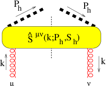
FIG. 3.: The gluon correlator

The procedure to analyse the gluon fragmentation functions is very similar to what has been done for the distributions in the previous sections.

Using as parameterization of the vectors

$$P_{h} = P_{h}^{-}n_{\scriptscriptstyle-}+{M_{h}^{2}\over 2P_{h}^{-}}n_{\scriptscriptstyle+},$$ (71)

$$k = {P_{h}^{-}\over z}n_{\scriptscriptstyle-}+{z(k^{2}+{\mathchoice{{\hbox{\boldmath$\displaystyle k$}}}{{\hbox{\boldmath$\textstyle k$}}}{{\hbox{\boldmath$\scriptstyle k$}}}{{\hbox{\boldmath$\scriptscriptstyle k$}}}}_{\scriptscriptstyle T}^{2})\over 2P_{h}^{-}}n_{\scriptscriptstyle+}+k_{\scriptscriptstyle T},$$ (72)

$$S_{h} = S_{h\scriptscriptstyle L}{P_{h}^{-}\over M_{h}}n_{\scriptscriptstyle-}-S_{h\scriptscriptstyle L}{M_{h}\over 2P_{h}^{-}}n_{\scriptscriptstyle+}+S_{hT}.$$ (73)

for a gluon with momentum $k$ fragmenting into a hadron with momentum $P_{h}$ and spin $S_{h}$, we consider the soft part (see Fig. 3)

$$\hat{S}^{\mu\nu}(k;P_{h},S_{h})=\sum_{X}\int\frac{d^{4}\xi}{(2\pi)^{4}}\,e^{ik\cdot\xi}\,\langle 0|A^{\nu}(\xi)|P_{h},S_{h};X\rangle\langle P_{h},S_{h};X|A^{\mu}(0)|0\rangle,$$ (74)

or the appropriate gauge-invariant object

$$\hat{\Gamma}^{\mu\nu;\rho\sigma}(k;P_{h},S_{h})=\sum_{X}\int\frac{d^{4}\xi}{(2\pi)^{4}}\,e^{ik\cdot\xi}\,\langle 0|F^{\rho\sigma}(\xi)|P_{h},S_{h};X\rangle\langle P_{h},S_{h};X|{\cal U}(\xi,0)\,F^{\mu\nu}(0)|0\rangle.$$ (75)

For the description of fragmentation in leading order in the inverse hard scale, we need this correlation function integrated over one lightcone direction, with the above choice for $P_{h}$, being the momentum $k^{+}$,

$$M_{h}\hat{\Gamma}^{ij}(z,\mathchoice{{\hbox{\boldmath$\displaystyle k$}}}{{\hbox{\boldmath$\textstyle k$}}}{{\hbox{\boldmath$\scriptstyle k$}}}{{\hbox{\boldmath$\scriptscriptstyle k$}}}_{\scriptscriptstyle T})=\int dk^{+}\ \Gamma^{-j;-i}(k;P_{h},S_{h}),$$ (76)

which, separating the polarizations, is parameterized as

$$\hat{\Gamma}_{O}^{ij}(z,{\mathchoice{{\hbox{\boldmath$\displaystyle k$}}}{{\hbox{\boldmath$\textstyle k$}}}{{\hbox{\boldmath$\scriptstyle k$}}}{{\hbox{\boldmath$\scriptscriptstyle k$}}}}_{\scriptscriptstyle T}) = {P_{h}^{-}\over M_{h}}\left[-g^{ij}_{\scriptscriptstyle T}\hat{G}(z,{\mathchoice{{\hbox{\boldmath$\displaystyle k$}}}{{\hbox{\boldmath$\textstyle k$}}}{{\hbox{\boldmath$\scriptstyle k$}}}{{\hbox{\boldmath$\scriptscriptstyle k$}}}}_{\scriptscriptstyle T}^{\prime 2})+\left({k_{\scriptscriptstyle T}^{i}k_{\scriptscriptstyle T}^{j}\over M_{h}^{2}}+g^{ij}_{\scriptscriptstyle T}{{\mathchoice{{\hbox{\boldmath$\displaystyle k$}}}{{\hbox{\boldmath$\textstyle k$}}}{{\hbox{\boldmath$\scriptstyle k$}}}{{\hbox{\boldmath$\scriptscriptstyle k$}}}}_{\scriptscriptstyle T}^{2}\over 2M_{h}^{2}}\right)\hat{H}^{\perp}(z,{\mathchoice{{\hbox{\boldmath$\displaystyle k$}}}{{\hbox{\boldmath$\textstyle k$}}}{{\hbox{\boldmath$\scriptstyle k$}}}{{\hbox{\boldmath$\scriptscriptstyle k$}}}}_{\scriptscriptstyle T}^{\prime 2})\right],$$ (77)

$$\hat{\Gamma}_{L}^{ij}(z,{\mathchoice{{\hbox{\boldmath$\displaystyle k$}}}{{\hbox{\boldmath$\textstyle k$}}}{{\hbox{\boldmath$\scriptstyle k$}}}{{\hbox{\boldmath$\scriptscriptstyle k$}}}}_{\scriptscriptstyle T}) = {P_{h}^{-}\over M_{h}}\left[i\epsilon^{ij}_{\scriptscriptstyle T}S_{h\scriptscriptstyle L}\ \Delta\hat{G}_{L}(z,{\mathchoice{{\hbox{\boldmath$\displaystyle k$}}}{{\hbox{\boldmath$\textstyle k$}}}{{\hbox{\boldmath$\scriptstyle k$}}}{{\hbox{\boldmath$\scriptscriptstyle k$}}}}_{\scriptscriptstyle T}^{\prime 2})-{\epsilon_{\scriptscriptstyle T}^{k_{\scriptscriptstyle T}\left\{i\right.}k_{\scriptscriptstyle T}^{\left.j\right\}}\over 2M_{h}^{2}}\ S_{h\scriptscriptstyle L}\ \Delta\hat{H}_{L}^{\perp}(z,{\mathchoice{{\hbox{\boldmath$\displaystyle k$}}}{{\hbox{\boldmath$\textstyle k$}}}{{\hbox{\boldmath$\scriptstyle k$}}}{{\hbox{\boldmath$\scriptscriptstyle k$}}}}_{\scriptscriptstyle T}^{\prime 2})\right],$$ (78)

$$\hat{\Gamma}_{T}^{ij}(z,{\mathchoice{{\hbox{\boldmath$\displaystyle k$}}}{{\hbox{\boldmath$\textstyle k$}}}{{\hbox{\boldmath$\scriptstyle k$}}}{{\hbox{\boldmath$\scriptscriptstyle k$}}}}_{\scriptscriptstyle T}) = {P_{h}^{-}\over M_{h}}\Biggl{[}g^{ij}_{\scriptscriptstyle T}\ {\epsilon_{\scriptscriptstyle T}^{k_{\scriptscriptstyle T}S_{\scriptscriptstyle hT}}\over M_{h}}\ \hat{G}_{T}(z,{\mathchoice{{\hbox{\boldmath$\displaystyle k$}}}{{\hbox{\boldmath$\textstyle k$}}}{{\hbox{\boldmath$\scriptstyle k$}}}{{\hbox{\boldmath$\scriptscriptstyle k$}}}}_{\scriptscriptstyle T}^{\prime 2})+i\epsilon^{ij}_{\scriptscriptstyle T}\ {{\mathchoice{{\hbox{\boldmath$\displaystyle k$}}}{{\hbox{\boldmath$\textstyle k$}}}{{\hbox{\boldmath$\scriptstyle k$}}}{{\hbox{\boldmath$\scriptscriptstyle k$}}}}_{\scriptscriptstyle T}\cdot{\mathchoice{{\hbox{\boldmath$\displaystyle S$}}}{{\hbox{\boldmath$\textstyle S$}}}{{\hbox{\boldmath$\scriptstyle S$}}}{{\hbox{\boldmath$\scriptscriptstyle S$}}}}_{hT}\over M_{h}}\ \Delta\hat{G}_{T}(z,{\mathchoice{{\hbox{\boldmath$\displaystyle k$}}}{{\hbox{\boldmath$\textstyle k$}}}{{\hbox{\boldmath$\scriptstyle k$}}}{{\hbox{\boldmath$\scriptscriptstyle k$}}}}_{\scriptscriptstyle T}^{\prime 2})$$ (81)

$$\qquad\quad-{\epsilon_{\scriptscriptstyle T}^{k_{\scriptscriptstyle T}\{i}k_{\scriptscriptstyle T}^{j\}}\over 2M_{h}^{2}}{{\mathchoice{{\hbox{\boldmath$\displaystyle k$}}}{{\hbox{\boldmath$\textstyle k$}}}{{\hbox{\boldmath$\scriptstyle k$}}}{{\hbox{\boldmath$\scriptscriptstyle k$}}}}_{\scriptscriptstyle T}\cdot{\mathchoice{{\hbox{\boldmath$\displaystyle S$}}}{{\hbox{\boldmath$\textstyle S$}}}{{\hbox{\boldmath$\scriptstyle S$}}}{{\hbox{\boldmath$\scriptscriptstyle S$}}}}_{hT}\over M_{h}}\ \Delta\hat{H}_{T}^{\perp}(z,{\mathchoice{{\hbox{\boldmath$\displaystyle k$}}}{{\hbox{\boldmath$\textstyle k$}}}{{\hbox{\boldmath$\scriptstyle k$}}}{{\hbox{\boldmath$\scriptscriptstyle k$}}}}_{\scriptscriptstyle T}^{\prime 2})$$

$$\qquad\quad-{\epsilon_{\scriptscriptstyle T}^{k_{\scriptscriptstyle T}\left\{i\right.}S_{\scriptscriptstyle hT}^{\left.j\right\}}+\epsilon_{\scriptscriptstyle T}^{S_{\scriptscriptstyle hT}\left\{i\right.}k_{\scriptscriptstyle T}^{\left.j\right\}}\over 4M_{h}}\,\left[\Delta\hat{H}_{T}(z,{\mathchoice{{\hbox{\boldmath$\displaystyle k$}}}{{\hbox{\boldmath$\textstyle k$}}}{{\hbox{\boldmath$\scriptstyle k$}}}{{\hbox{\boldmath$\scriptscriptstyle k$}}}}_{\scriptscriptstyle T}^{\prime 2})-\frac{{\mathchoice{{\hbox{\boldmath$\displaystyle k$}}}{{\hbox{\boldmath$\textstyle k$}}}{{\hbox{\boldmath$\scriptstyle k$}}}{{\hbox{\boldmath$\scriptscriptstyle k$}}}}_{\scriptscriptstyle T}^{2}}{2M^{2}}\,\Delta\hat{H}_{T}^{\perp}(z,{\mathchoice{{\hbox{\boldmath$\displaystyle k$}}}{{\hbox{\boldmath$\textstyle k$}}}{{\hbox{\boldmath$\scriptstyle k$}}}{{\hbox{\boldmath$\scriptscriptstyle k$}}}}_{\scriptscriptstyle T}^{\prime 2})\right]\Biggr{]},$$

where the argument of the fragmentation functions, $\mathchoice{{\hbox{\boldmath$\displaystyle k$}}}{{\hbox{\boldmath$\textstyle k$}}}{{\hbox{\boldmath$\scriptstyle k$}}}{{\hbox{\boldmath$\scriptscriptstyle k$}}}_{\scriptscriptstyle T}^{\prime}=-z\mathchoice{{\hbox{\boldmath$\displaystyle k$}}}{{\hbox{\boldmath$\textstyle k$}}}{{\hbox{\boldmath$\scriptstyle k$}}}{{\hbox{\boldmath$\scriptscriptstyle k$}}}_{\scriptscriptstyle T}$ is the transverse momentum of the hadron with respect to the gluon. The factors are chosen such that $\int dz\,d^{2}k_{\scriptscriptstyle T}^{\prime}\ z\hat{G}(z,{\mathchoice{{\hbox{\boldmath$\displaystyle k$}}}{{\hbox{\boldmath$\textstyle k$}}}{{\hbox{\boldmath$\scriptstyle k$}}}{{\hbox{\boldmath$\scriptscriptstyle k$}}}}_{\scriptscriptstyle T}^{\prime 2})=\langle z\rangle_{h}$ is the fraction of momentum of the struck gluon taken by the hadron $h$, for which we have $\sum_{h}\langle z\rangle_{h}=1$. While for distribution functions T-odd functions might appear via special mechanisms dealing with initial state interactions or gluonic poles, this is not the case for fragmentation functions [13, 14], where time-reversal symmetry cannot be used as a constraint because of the explicit appearance of out states $|P_{h};X\rangle$ in the definition. Thus one expects nonvanishing fragmentation functions $\hat{G}_{T}(z,{\mathchoice{{\hbox{\boldmath$\displaystyle k$}}}{{\hbox{\boldmath$\textstyle k$}}}{{\hbox{\boldmath$\scriptstyle k$}}}{{\hbox{\boldmath$\scriptscriptstyle k$}}}}_{\scriptscriptstyle T}^{\prime 2})$, $\Delta\hat{H}_{L}^{\perp}(z,{\mathchoice{{\hbox{\boldmath$\displaystyle k$}}}{{\hbox{\boldmath$\textstyle k$}}}{{\hbox{\boldmath$\scriptstyle k$}}}{{\hbox{\boldmath$\scriptscriptstyle k$}}}}_{\scriptscriptstyle T}^{\prime 2})$, $\Delta\hat{H}_{T}^{\perp}(z,{\mathchoice{{\hbox{\boldmath$\displaystyle k$}}}{{\hbox{\boldmath$\textstyle k$}}}{{\hbox{\boldmath$\scriptstyle k$}}}{{\hbox{\boldmath$\scriptscriptstyle k$}}}}_{\scriptscriptstyle T}^{\prime 2})$ and $\Delta\hat{H}_{T}(z,{\mathchoice{{\hbox{\boldmath$\displaystyle k$}}}{{\hbox{\boldmath$\textstyle k$}}}{{\hbox{\boldmath$\scriptstyle k$}}}{{\hbox{\boldmath$\scriptscriptstyle k$}}}}_{\scriptscriptstyle T}^{\prime 2})$.

V Bounds on the distribution and fragmentation functions

As discussed before, we can organize the distribution functions in a matrix representation in the gluon $\otimes$ nucleon spin space. For distribution functions one has (omitting the T-odd functions) a matrix

$$\frac{2}{x}\,\frac{M}{P^{+}}\,\Gamma(x,{\mathchoice{{\hbox{\boldmath$\displaystyle k$}}}{{\hbox{\boldmath$\textstyle k$}}}{{\hbox{\boldmath$\scriptstyle k$}}}{{\hbox{\boldmath$\scriptscriptstyle k$}}}}_{\scriptscriptstyle T})=\left(\begin{array}[]{cccc}G+\Delta G_{L}&{|{\mathchoice{{\hbox{\boldmath$\displaystyle k$}}}{{\hbox{\boldmath$\textstyle k$}}}{{\hbox{\boldmath$\scriptstyle k$}}}{{\hbox{\boldmath$\scriptscriptstyle k$}}}}_{\scriptscriptstyle T}|e^{-i\phi}\over M}\ \Delta G_{T}&-e^{-2i\phi}\ H^{\perp(1)}&0\\ {|{\mathchoice{{\hbox{\boldmath$\displaystyle k$}}}{{\hbox{\boldmath$\textstyle k$}}}{{\hbox{\boldmath$\scriptstyle k$}}}{{\hbox{\boldmath$\scriptscriptstyle k$}}}}_{\scriptscriptstyle T}|e^{i\phi}\over M}\ \Delta G_{T}&G-\Delta G_{L}&0&-e^{-2i\phi}\ H^{\perp(1)}\\ -e^{2i\phi}\ H^{\perp(1)}&0&G-\Delta G_{L}&-{|{\mathchoice{{\hbox{\boldmath$\displaystyle k$}}}{{\hbox{\boldmath$\textstyle k$}}}{{\hbox{\boldmath$\scriptstyle k$}}}{{\hbox{\boldmath$\scriptscriptstyle k$}}}}_{\scriptscriptstyle T}|e^{-i\phi}\over M}\ \Delta G_{T}\\ 0&-e^{2i\phi}\ H^{\perp(1)}&-{|{\mathchoice{{\hbox{\boldmath$\displaystyle k$}}}{{\hbox{\boldmath$\textstyle k$}}}{{\hbox{\boldmath$\scriptstyle k$}}}{{\hbox{\boldmath$\scriptscriptstyle k$}}}}_{\scriptscriptstyle T}|e^{i\phi}\over M}\ \Delta G_{T}&G+\Delta G_{L}\end{array}\right).$$ (82)

Requiring any diagonal element to be positive gives using the diagonal elements the trivial bound

$$|\Delta G_{L}(x,{\mathchoice{{\hbox{\boldmath$\displaystyle k$}}}{{\hbox{\boldmath$\textstyle k$}}}{{\hbox{\boldmath$\scriptstyle k$}}}{{\hbox{\boldmath$\scriptscriptstyle k$}}}}_{\scriptscriptstyle T}^{2})|\leq G(x,{\mathchoice{{\hbox{\boldmath$\displaystyle k$}}}{{\hbox{\boldmath$\textstyle k$}}}{{\hbox{\boldmath$\scriptstyle k$}}}{{\hbox{\boldmath$\scriptscriptstyle k$}}}}_{\scriptscriptstyle T}^{2}).$$ (83)

Using all possible 2 $\times$ 2 submatrices, positivity leads to bounds

$$|\Delta G_{T}^{(1)}|\leq\frac{|{\mathchoice{{\hbox{\boldmath$\displaystyle k$}}}{{\hbox{\boldmath$\textstyle k$}}}{{\hbox{\boldmath$\scriptstyle k$}}}{{\hbox{\boldmath$\scriptscriptstyle k$}}}}_{\scriptscriptstyle T}|}{2M}\,\sqrt{(G+\Delta G_{L})(G-\Delta G_{L})}\leq\frac{|{\mathchoice{{\hbox{\boldmath$\displaystyle k$}}}{{\hbox{\boldmath$\textstyle k$}}}{{\hbox{\boldmath$\scriptstyle k$}}}{{\hbox{\boldmath$\scriptscriptstyle k$}}}}_{\scriptscriptstyle T}|}{2M}\,G,$$ (84)

$$|H^{\perp(1)}|\leq\sqrt{(G+\Delta G_{L})(G-\Delta G_{L})}\leq G.$$ (85)

These bounds can still be sharpened by using the eigenvalues of the full 4 $\times$ 4 matrix in analogy to what was done for quark distributions in Ref. [15].

For fragmentation functions the matrix $(M_{h}/P_{h}^{-})\,\hat{\Gamma}(z,\mathchoice{{\hbox{\boldmath$\displaystyle k$}}}{{\hbox{\boldmath$\textstyle k$}}}{{\hbox{\boldmath$\scriptstyle k$}}}{{\hbox{\boldmath$\scriptscriptstyle k$}}}_{\scriptscriptstyle T})$ contains the various fragmentation functions, now including the T-odd functions. It thus is the same as the matrix in 70, but with hat functions depending on $z$ and $\mathchoice{{\hbox{\boldmath$\displaystyle k$}}}{{\hbox{\boldmath$\textstyle k$}}}{{\hbox{\boldmath$\scriptstyle k$}}}{{\hbox{\boldmath$\scriptscriptstyle k$}}}_{\scriptscriptstyle T}^{\prime}$. The constraints become

$$|\Delta\hat{G}_{L}(z,{\mathchoice{{\hbox{\boldmath$\displaystyle k$}}}{{\hbox{\boldmath$\textstyle k$}}}{{\hbox{\boldmath$\scriptstyle k$}}}{{\hbox{\boldmath$\scriptscriptstyle k$}}}}_{\scriptscriptstyle T}^{\prime 2})|\leq\hat{G}(z,{\mathchoice{{\hbox{\boldmath$\displaystyle k$}}}{{\hbox{\boldmath$\textstyle k$}}}{{\hbox{\boldmath$\scriptstyle k$}}}{{\hbox{\boldmath$\scriptscriptstyle k$}}}}_{\scriptscriptstyle T}^{\prime 2}),$$ (86)

$$|\Delta\hat{G}_{T}^{(1)}|^{2}+|\hat{G}_{T}^{(1)}|^{2}\leq\frac{|k_{\scriptscriptstyle T}|^{2}}{4M_{h}^{2}}\,(\hat{G}+\Delta\hat{G}_{L})(\hat{G}-\Delta\hat{G}_{L})\leq\frac{|k_{\scriptscriptstyle T}|^{2}}{4M_{h}^{2}}\,\hat{G}^{2},$$ (87)

$$|\hat{H}^{\perp(1)}|^{2}+|\Delta\hat{H}_{L}^{\perp(1)}|^{2}\leq(\hat{G}+\Delta\hat{G}_{L})(\hat{G}-\Delta\hat{G}_{L})\leq\hat{G}^{2},$$ (88)

$$|\Delta\hat{H}_{T}^{\perp(2)}|\leq\frac{|{\mathchoice{{\hbox{\boldmath$\displaystyle k$}}}{{\hbox{\boldmath$\textstyle k$}}}{{\hbox{\boldmath$\scriptstyle k$}}}{{\hbox{\boldmath$\scriptscriptstyle k$}}}}_{\scriptscriptstyle T}|}{2M_{h}}\,(\hat{G}+\Delta\hat{G}_{L}),$$ (89)

$$|\Delta\hat{H}_{T}^{(1)}|\leq\frac{|{\mathchoice{{\hbox{\boldmath$\displaystyle k$}}}{{\hbox{\boldmath$\textstyle k$}}}{{\hbox{\boldmath$\scriptstyle k$}}}{{\hbox{\boldmath$\scriptscriptstyle k$}}}}_{\scriptscriptstyle T}|}{2M_{h}}\,(\hat{G}-\Delta\hat{G}_{L}).$$ (90)

VI Conclusions

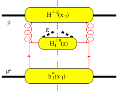
(a)

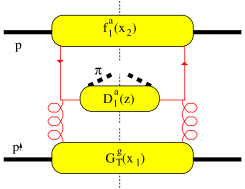
(b)

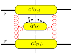
(c)

FIG. 4.: Gluon distribution and fragmentation functions contributing to the single spin asymmetry in $p^{\uparrow}p\rightarrow\pi X$ scattering cross section.

We have given a full classification of the gluon distributions and fragmentation functions relevant in hard scattering processes in leading order in the inverse hard scale including transverse momentum dependence. Some results for subleading (twist three) correlation functions have been given also. The inclusion of transverse momentum dependence is needed in processes involving at least two hadrons. Examples of such processes are 1-particle inclusive leptoproduction or Drell-Yan scattering. In these processes one can become sensitive to transverse momentum dependence, in particular when one considers azimuthal dependence in the final state [1, 2, 10, 16]. We note that in electroweak processes, the gluon correlation functions do not enter at tree level but only at higher order in $\alpha_{s}$. This also implies their relevance in the study of evolution of the transverse momentum dependent flavor-singlet quark distribution and fragmentation functions. Also in related processes, e.g. $\chi_{2}$-production in hadron-hadron scattering the relevance of gluon distribution functions has been emphasized and investigated [6]. Since we have discussed both distribution and fragmentation functions we have also classified the T-odd functions, important in the latter case. In single spin asymmetries at least one of the functions describing the soft physics is a T-odd function.

In order to illustrate the importance of also considering gluons, we consider the contributions to pion production in $pp^{\uparrow}$ scattering in which one of the protons is polarized [17, 18, 19, 20, 21]. In this process a large single spin asymmetry is found. We note that gluon correlation functions can play an important role here. This is another way of looking to the approach in Refs. [18, 19, 20, 21]. Since in this case several mechanisms are considered in these papers, we need both T-odd and T-even distribution and fragmentation functions. In Fig. 4 three contributions are shown of gluon correlation functions producing an asymmetry. Actually kinematics requires one of the three partons to be off-shell, which means that we need the asymptotic transverse momentum dependence of the soft parts, i.e. the evolution of the soft parts. Nevertheless the structure of the gluonic soft parts is sufficient to indicate that diagram (4a) will produce a $\sin(\phi_{\pi}+\phi_{S})$ asymmetry (being equivalent to the Collins asymmetry in leptoproduction). This asymmetry is proportional to $(h_{1}^{a}(x_{1})\times H^{\perp}(x_{2}))\times\hat{h}_{1}^{\perp}(z)$ involving the transverse momentum dependent gluon distribution function $H^{\perp}$, the transverse spin distribution $h_{1}^{a}$ and the Collins function $\hat{h}_{1}^{\perp}$ (we use here the hat-notation for the fragmentation function in order to avoid confusion between fragmentation functions and gluon distribution functions). Diagram (4b) will lead to a $\sin(\phi_{\pi}-\phi_{S})$ asymmetry proportional to $(G_{T}(x_{1})\times f_{1}^{a}(x_{2}))\times D_{1}^{a}(z)$ involving a T-odd gluon distribution function, the unpolarized quark distribution function $f_{1}^{a}$ and fragmentation function $D_{1}^{a}$. Diagram (4c) gives a similar asymmetry as (4b) with the unpolarized gluon distribution function $G$ and gluon fragmentation function $\hat{G}$.

A Gluon Distributions

Leading and subleading gluon correlations are distinguished via the Lorentz indices. It is therefore convenient to rewrite the covariant expression in Eq. 16 in terms of $(n_{\scriptscriptstyle+},n_{\scriptscriptstyle-},{\mathchoice{{\hbox{\boldmath$\displaystyle k$}}}{{\hbox{\boldmath$\textstyle k$}}}{{\hbox{\boldmath$\scriptstyle k$}}}{{\hbox{\boldmath$\scriptscriptstyle k$}}}}_{\scriptscriptstyle T},{\mathchoice{{\hbox{\boldmath$\displaystyle S$}}}{{\hbox{\boldmath$\textstyle S$}}}{{\hbox{\boldmath$\scriptstyle S$}}}{{\hbox{\boldmath$\scriptscriptstyle S$}}}}_{\scriptscriptstyle T})$. We start with the correlation functions with the maximal (that is two) number of plus indices. Distinguishing unpolarized (O), longitudinally polarized (L) and transversely polarized (T) situations (spin 1/2),

$$\Gamma^{+\mu;+\nu}=\Gamma_{O}^{+\mu;+\nu}+\Gamma_{L}^{+\mu;+\nu}+\Gamma_{T}^{+\mu;+\nu},$$ (A1)

one has, with the (dimensionless) invariants $\sigma=2k\cdot P/M^{2}$ and $\tau=k^{2}/M^{2}$, the result

$$\Gamma_{O}^{+\mu;+\nu} = \left({P^{+}\over M}\right)^{2}(-g^{\mu\nu}_{\scriptscriptstyle T})\left[(X_{2}+xX_{4})+x(X_{4}+xX_{3})\right]+\left({P^{+}\over M}\right)^{2}{k_{\scriptscriptstyle T}^{\mu}k_{\scriptscriptstyle T}^{\nu}\over M^{2}}\ X_{6}$$ (A4)

$$+{P^{+}\over M}\ {k_{\scriptscriptstyle T}^{\left\{\mu\right.}n_{\scriptscriptstyle-}^{\left.\nu\right\}}\over M}\left[(X_{4}+xX_{3})+\left({\sigma\over 2}-x\right)X_{6}\right]-{P^{+}\over M}\ {k_{\scriptscriptstyle T}^{\left[\mu\right.}n_{\scriptscriptstyle-}^{\left.\nu\right]}\over M}\ iX_{5}$$

$$+n_{\scriptscriptstyle-}^{\mu}n_{\scriptscriptstyle-}^{\nu}\left[2X_{1}+[(X_{2}+xX_{4})+x(X_{4}+xX_{3})]+2\left({\sigma\over 2}-x\right)(X_{4}+xX_{3})+\left({\sigma\over 2}-x\right)^{2}X_{6}\right],$$

$$\Gamma_{L}^{+\mu;+\nu} = iS_{\scriptscriptstyle L}\left({P^{+}\over M}\right)^{2}\epsilon^{\mu\nu}_{\scriptscriptstyle T}\left\{(X_{8}+xX_{10})+(X_{9}+xX_{11})+\left({\sigma\over 2}-x\right)\left[(X_{12}+xX_{14})+x(X_{15}+xX_{13})\right]\right.$$ (A10)

$$\left.-{{\mathchoice{{\hbox{\boldmath$\displaystyle k$}}}{{\hbox{\boldmath$\textstyle k$}}}{{\hbox{\boldmath$\scriptstyle k$}}}{{\hbox{\boldmath$\scriptscriptstyle k$}}}}_{\scriptscriptstyle T}^{2}\over M^{2}}\left[X_{19}+X_{23}+\left({\sigma\over 2}-x\right)X_{25}\right]\right\}$$

$$+S_{\scriptscriptstyle L}\left({P^{+}\over M}\right)^{2}{\epsilon_{\scriptscriptstyle T}^{k_{\scriptscriptstyle T}\left\{\mu\right.}k_{\scriptscriptstyle T}^{\left.\nu\right\}}\over M^{2}}\left[-(X_{18}+X_{22})-\left({\sigma\over 2}-x\right)X_{24}\right]$$

$$+iS_{\scriptscriptstyle L}\ {P^{+}\over M}\ {\epsilon^{k_{\scriptscriptstyle T}\left[\mu\right.}n_{\scriptscriptstyle-}^{\left.\nu\right]}\over M}\left[X_{10}+\left({\sigma\over 2}-x\right)(X_{15}+xX_{13})\right.$$

$$\left.-\left({\sigma\over 2}-x\right)(X_{19}+X_{23})-(X_{21}+xX_{23})-\left({\sigma\over 2}-x\right)^{2}X_{25}\right]$$

$$+S_{\scriptscriptstyle L}\ {P^{+}\over M}{\epsilon_{\scriptscriptstyle T}^{k_{\scriptscriptstyle T}\left\{\mu\right.}n_{\scriptscriptstyle-}^{\left.\nu\right\}}\over M}\left[-\left({\sigma\over 2}-x\right)(X_{18}+X_{22})-(X_{20}+xX_{22})-\left({\sigma\over 2}-x\right)^{2}X_{24}\right],$$

$$\Gamma_{T}^{+\mu;+\nu} = i\left({P^{+}\over M}\right)^{2}{{\mathchoice{{\hbox{\boldmath$\displaystyle k$}}}{{\hbox{\boldmath$\textstyle k$}}}{{\hbox{\boldmath$\scriptstyle k$}}}{{\hbox{\boldmath$\scriptscriptstyle k$}}}}_{\scriptscriptstyle T}\cdot{\mathchoice{{\hbox{\boldmath$\displaystyle S$}}}{{\hbox{\boldmath$\textstyle S$}}}{{\hbox{\boldmath$\scriptstyle S$}}}{{\hbox{\boldmath$\scriptscriptstyle S$}}}}_{\scriptscriptstyle T}\over M}\ \epsilon^{\mu\nu}_{\scriptscriptstyle T}\left[-(X_{12}+xX_{14})-x(X_{15}+xX_{13})\right.$$ (A17)

$$\left.+(X_{17}+xX_{19})+(X_{21}+xX_{23})+{{\mathchoice{{\hbox{\boldmath$\displaystyle k$}}}{{\hbox{\boldmath$\textstyle k$}}}{{\hbox{\boldmath$\scriptstyle k$}}}{{\hbox{\boldmath$\scriptscriptstyle k$}}}}_{\scriptscriptstyle T}^{2}\over M^{2}}\ X_{25}\right]$$

$$+\left({P^{+}\over M}\right)^{2}\left\{{\epsilon_{T}^{k_{\scriptscriptstyle T}\left\{\mu\right.}k_{\scriptscriptstyle T}^{\left.\nu\right\}}\over M^{2}}\ {{\mathchoice{{\hbox{\boldmath$\displaystyle k$}}}{{\hbox{\boldmath$\textstyle k$}}}{{\hbox{\boldmath$\scriptstyle k$}}}{{\hbox{\boldmath$\scriptscriptstyle k$}}}}_{\scriptscriptstyle T}\cdot{\mathchoice{{\hbox{\boldmath$\displaystyle S$}}}{{\hbox{\boldmath$\textstyle S$}}}{{\hbox{\boldmath$\scriptstyle S$}}}{{\hbox{\boldmath$\scriptscriptstyle S$}}}}_{\scriptscriptstyle T}\over M}\ X_{24}+{\epsilon_{T}^{k_{\scriptscriptstyle T}\left\{\mu\right.}S_{\scriptscriptstyle T}^{\left.\nu\right\}}\over M}\left(X_{20}+xX_{22}\right)+{\epsilon_{T}^{S_{\scriptscriptstyle T}\left\{\mu\right.}k_{\scriptscriptstyle T}^{\left.\nu\right\}}\over M}\left(X_{16}+xX_{18}\right)\right\}$$

$$+i{P^{+}\over M}\left\{{\epsilon_{\scriptscriptstyle T}^{k_{\scriptscriptstyle T}\left[\mu\right.}n_{\scriptscriptstyle-}^{\left.\nu\right]}\over M}\ {{\mathchoice{{\hbox{\boldmath$\displaystyle k$}}}{{\hbox{\boldmath$\textstyle k$}}}{{\hbox{\boldmath$\scriptstyle k$}}}{{\hbox{\boldmath$\scriptscriptstyle k$}}}}_{\scriptscriptstyle T}\cdot{\mathchoice{{\hbox{\boldmath$\displaystyle S$}}}{{\hbox{\boldmath$\textstyle S$}}}{{\hbox{\boldmath$\scriptstyle S$}}}{{\hbox{\boldmath$\scriptscriptstyle S$}}}}_{\scriptscriptstyle T}\over M}\left[-(X_{15}+xX_{13})+X_{19}+\left({\sigma\over 2}-x\right)X_{25}\right]\right.$$

$$\left.+\epsilon_{\scriptscriptstyle T}^{S_{\scriptscriptstyle T}\left[\mu\right.}n_{\scriptscriptstyle-}^{\left.\nu\right]}\left[(X_{9}+xX_{11})+\left({\sigma\over 2}-x\right)(X_{17}+xX_{19})-{{\mathchoice{{\hbox{\boldmath$\displaystyle k$}}}{{\hbox{\boldmath$\textstyle k$}}}{{\hbox{\boldmath$\scriptstyle k$}}}{{\hbox{\boldmath$\scriptscriptstyle k$}}}}_{\scriptscriptstyle T}^{2}\over M^{2}}\ X_{19}\right]\right\}$$

$$+{P^{+}\over M}\left\{{\epsilon_{T}^{k_{\scriptscriptstyle T}\left\{\mu\right.}n_{\scriptscriptstyle-}^{\left.\nu\right\}}\over M}\ {{\mathchoice{{\hbox{\boldmath$\displaystyle k$}}}{{\hbox{\boldmath$\textstyle k$}}}{{\hbox{\boldmath$\scriptstyle k$}}}{{\hbox{\boldmath$\scriptscriptstyle k$}}}}_{\scriptscriptstyle T}\cdot{\mathchoice{{\hbox{\boldmath$\displaystyle S$}}}{{\hbox{\boldmath$\textstyle S$}}}{{\hbox{\boldmath$\scriptstyle S$}}}{{\hbox{\boldmath$\scriptscriptstyle S$}}}}_{\scriptscriptstyle T}\over M}\left({\sigma\over 2}-x\right)X_{24}+\epsilon_{\scriptscriptstyle T}^{S_{\scriptscriptstyle T}\left\{\mu\right.}n_{\scriptscriptstyle-}^{\left.\nu\right\}}\left({\sigma\over 2}-x\right)(X_{16}+xX_{18})-{\epsilon^{n_{\scriptscriptstyle-}k_{\scriptscriptstyle T}S_{\scriptscriptstyle T}\left\{\mu\right.}k_{\scriptscriptstyle T}^{\left.\nu\right\}}\over M^{2}}\ X_{18}\right\}$$

$$-{\epsilon^{n_{\scriptscriptstyle-}k_{\scriptscriptstyle T}S_{\scriptscriptstyle T}\left\{\mu\right.}n_{\scriptscriptstyle-}^{\left.\nu\right\}}\over M}\left({\sigma\over 2}-x\right)X_{18},$$

We need the soft parts integrated over the momentum component $k^{-}$. Upon integration over $dk^{-}$ we find that the functions appearing in the decomposition of the quantity $M\Gamma^{ij}$ in Eq. 23 can be expressed in the amplitudes of Eq. 16. For this we use

$$M\Gamma^{ij}(x,{\mathchoice{{\hbox{\boldmath$\displaystyle k$}}}{{\hbox{\boldmath$\textstyle k$}}}{{\hbox{\boldmath$\scriptstyle k$}}}{{\hbox{\boldmath$\scriptscriptstyle k$}}}}_{\scriptscriptstyle T};P,S)\equiv\int dk^{-}\ \Gamma^{+i;+j}(k;P,S)={M^{2}\over 2P^{+}}\ \int[d\sigma d\tau]\ \Gamma^{+i;+j}(k;P,S),$$ (A18)

where we have introduced the shorthand notation

$$[d\sigma d\tau]\equiv d\sigma d\tau\ \delta\left(\tau-x\sigma+x^{2}+{{\mathchoice{{\hbox{\boldmath$\displaystyle k$}}}{{\hbox{\boldmath$\textstyle k$}}}{{\hbox{\boldmath$\scriptstyle k$}}}{{\hbox{\boldmath$\scriptscriptstyle k$}}}}_{\scriptscriptstyle T}^{2}\over M^{2}}\right),$$ (A19)

to indicate integration over $\sigma$ and $\tau$. The results for the twist two distributions in terms of the amplitudes $X_{i}$ are the following:

$$xG(x,{\mathchoice{{\hbox{\boldmath$\displaystyle k$}}}{{\hbox{\boldmath$\textstyle k$}}}{{\hbox{\boldmath$\scriptstyle k$}}}{{\hbox{\boldmath$\scriptscriptstyle k$}}}}_{\scriptscriptstyle T}^{2}) = \int[d\sigma d\tau]\ \left[[(X_{2}+xX_{4})+x(X_{4}+xX_{3})]+{{\mathchoice{{\hbox{\boldmath$\displaystyle k$}}}{{\hbox{\boldmath$\textstyle k$}}}{{\hbox{\boldmath$\scriptstyle k$}}}{{\hbox{\boldmath$\scriptscriptstyle k$}}}}_{\scriptscriptstyle T}^{2}\over 2M^{2}}\ X_{6}\right],$$ (A20)

$$xG_{T}(x,{\mathchoice{{\hbox{\boldmath$\displaystyle k$}}}{{\hbox{\boldmath$\textstyle k$}}}{{\hbox{\boldmath$\scriptstyle k$}}}{{\hbox{\boldmath$\scriptscriptstyle k$}}}}_{\scriptscriptstyle T}^{2}) = \int[d\sigma d\tau]\ \left[(X_{16}+xX_{18})-(X_{20}+xX_{22})\right],$$ (A21)

$$xH^{\perp}(x,{\mathchoice{{\hbox{\boldmath$\displaystyle k$}}}{{\hbox{\boldmath$\textstyle k$}}}{{\hbox{\boldmath$\scriptstyle k$}}}{{\hbox{\boldmath$\scriptscriptstyle k$}}}}_{\scriptscriptstyle T}^{2}) = \int[d\sigma d\tau]\ X_{6},$$ (A22)

$$x\Delta G_{L}(x,{\mathchoice{{\hbox{\boldmath$\displaystyle k$}}}{{\hbox{\boldmath$\textstyle k$}}}{{\hbox{\boldmath$\scriptstyle k$}}}{{\hbox{\boldmath$\scriptscriptstyle k$}}}}_{\scriptscriptstyle T}^{2}) = -\int[d\sigma d\tau]\ \left[(X_{8}+xX_{10})+(X_{9}+xX_{11})+\left({\sigma\over 2}-x\right)[(X_{12}+xX_{14})+x(X_{15}+xX_{13})]\right.$$ (A24)

$$\left.-{{\mathchoice{{\hbox{\boldmath$\displaystyle k$}}}{{\hbox{\boldmath$\textstyle k$}}}{{\hbox{\boldmath$\scriptstyle k$}}}{{\hbox{\boldmath$\scriptscriptstyle k$}}}}_{\scriptscriptstyle T}^{2}\over M^{2}}\left[X_{19}+X_{23}+\left({\sigma\over 2}-x\right)X_{25}\right]\right],$$

$$x\Delta G_{T}(x,{\mathchoice{{\hbox{\boldmath$\displaystyle k$}}}{{\hbox{\boldmath$\textstyle k$}}}{{\hbox{\boldmath$\scriptstyle k$}}}{{\hbox{\boldmath$\scriptscriptstyle k$}}}}_{\scriptscriptstyle T}^{2}) = \int[d\sigma d\tau]\ \left[(X_{12}+xX_{14})+x(X_{15}+xX_{13})-(X_{17}+xX_{19})-(X_{21}+xX_{23})-{{\mathchoice{{\hbox{\boldmath$\displaystyle k$}}}{{\hbox{\boldmath$\textstyle k$}}}{{\hbox{\boldmath$\scriptstyle k$}}}{{\hbox{\boldmath$\scriptscriptstyle k$}}}}_{\scriptscriptstyle T}^{2}\over M^{2}}\ X_{25}\right],$$ (A25)

$$x\ \Delta H_{L}^{\perp}(x,{\mathchoice{{\hbox{\boldmath$\displaystyle k$}}}{{\hbox{\boldmath$\textstyle k$}}}{{\hbox{\boldmath$\scriptstyle k$}}}{{\hbox{\boldmath$\scriptscriptstyle k$}}}}_{\scriptscriptstyle T}^{2}) = -2\int[d\sigma d\tau]\ \left[(X_{18}+X_{22})+\left({\sigma\over 2}-x\right)X_{24}\right],$$ (A26)

$$x\Delta H_{T}^{\perp}(x,{\mathchoice{{\hbox{\boldmath$\displaystyle k$}}}{{\hbox{\boldmath$\textstyle k$}}}{{\hbox{\boldmath$\scriptstyle k$}}}{{\hbox{\boldmath$\scriptscriptstyle k$}}}}_{\scriptscriptstyle T}^{2}) = 2\int[d\sigma d\tau]\ X_{24},$$ (A27)

$$x\Delta H_{T}(x,{\mathchoice{{\hbox{\boldmath$\displaystyle k$}}}{{\hbox{\boldmath$\textstyle k$}}}{{\hbox{\boldmath$\scriptstyle k$}}}{{\hbox{\boldmath$\scriptscriptstyle k$}}}}_{\scriptscriptstyle T}^{2}) = 2\int[d\sigma d\tau]\ \left[(X_{16}+xX_{18})+(X_{20}+xX_{22})-{{\mathchoice{{\hbox{\boldmath$\displaystyle k$}}}{{\hbox{\boldmath$\textstyle k$}}}{{\hbox{\boldmath$\scriptstyle k$}}}{{\hbox{\boldmath$\scriptscriptstyle k$}}}}_{\scriptscriptstyle T}^{2}\over 2M^{2}}\ X_{24}\right].$$ (A28)

From Eq. A4 we can also obtain the relation between the functions in the first quantity, $M\Gamma^{i-}$, relevant at twist three. We find that all functions have a real part (which is T-even) and an imaginary part (which is T-odd):

$${\cal R}e\left(xG_{3}^{\perp}(x,{\mathchoice{{\hbox{\boldmath$\displaystyle k$}}}{{\hbox{\boldmath$\textstyle k$}}}{{\hbox{\boldmath$\scriptstyle k$}}}{{\hbox{\boldmath$\scriptscriptstyle k$}}}}_{\scriptscriptstyle T}^{2})\right) = \int[d\sigma d\tau]\ \left[(X_{4}+xX_{3})+\left({\sigma\over 2}-x\right)X_{6}\right],$$ (A29)

$${\cal I}m\left(xG_{3}^{\perp}(x,{\mathchoice{{\hbox{\boldmath$\displaystyle k$}}}{{\hbox{\boldmath$\textstyle k$}}}{{\hbox{\boldmath$\scriptstyle k$}}}{{\hbox{\boldmath$\scriptscriptstyle k$}}}}_{\scriptscriptstyle T}^{2})\right) = \int[d\sigma d\tau]\ \left[-X_{5}\right],$$ (A30)

$${\cal R}e\left(x\Delta G_{3L}^{\perp}(x,{\mathchoice{{\hbox{\boldmath$\displaystyle k$}}}{{\hbox{\boldmath$\textstyle k$}}}{{\hbox{\boldmath$\scriptstyle k$}}}{{\hbox{\boldmath$\scriptscriptstyle k$}}}}_{\scriptscriptstyle T}^{2})\right) = \int[d\sigma d\tau]\ \left[X_{10}+\left({\sigma\over 2}-x\right)(X_{15}+xX_{13})-\left({\sigma\over 2}-x\right)(X_{19}+X_{23})\right.$$ (A32)

$$\left.-(X_{21}+xX_{23})-\left({\sigma\over 2}-x\right)^{2}X_{25}\right],$$

$${\cal I}m\left(x\Delta G_{3L}^{\perp}(x,{\mathchoice{{\hbox{\boldmath$\displaystyle k$}}}{{\hbox{\boldmath$\textstyle k$}}}{{\hbox{\boldmath$\scriptstyle k$}}}{{\hbox{\boldmath$\scriptscriptstyle k$}}}}_{\scriptscriptstyle T}^{2})\right) = \int[d\sigma d\tau]\ \left[\left({\sigma\over 2}-x\right)(X_{18}+X_{22})+(X_{20}+xX_{22})+\left({\sigma\over 2}-x\right)^{2}X_{24}\right],$$ (A33)

$${\cal R}e\left(x\Delta G_{3T}(x,{\mathchoice{{\hbox{\boldmath$\displaystyle k$}}}{{\hbox{\boldmath$\textstyle k$}}}{{\hbox{\boldmath$\scriptstyle k$}}}{{\hbox{\boldmath$\scriptscriptstyle k$}}}}_{\scriptscriptstyle T}^{2})\right) = \int[d\sigma d\tau]\ \left[(X_{9}+xX_{11})+\left({\sigma\over 2}-x\right)(X_{17}+xX_{19})\right.$$ (A35)

$$\left.+{{\mathchoice{{\hbox{\boldmath$\displaystyle k$}}}{{\hbox{\boldmath$\textstyle k$}}}{{\hbox{\boldmath$\scriptstyle k$}}}{{\hbox{\boldmath$\scriptscriptstyle k$}}}}_{\scriptscriptstyle T}^{2}\over 2M^{2}}\left[-(X_{15}+xX_{13})-X_{19}+\left({\sigma\over 2}-x\right)X_{25}\right]\right],$$

$${\cal I}m\left(x\Delta G_{3T}(x,{\mathchoice{{\hbox{\boldmath$\displaystyle k$}}}{{\hbox{\boldmath$\textstyle k$}}}{{\hbox{\boldmath$\scriptstyle k$}}}{{\hbox{\boldmath$\scriptscriptstyle k$}}}}_{\scriptscriptstyle T}^{2})\right) = \int[d\sigma d\tau]\ \left[-\left({\sigma\over 2}-x\right)(X_{16}+xX_{18})-{{\mathchoice{{\hbox{\boldmath$\displaystyle k$}}}{{\hbox{\boldmath$\textstyle k$}}}{{\hbox{\boldmath$\scriptstyle k$}}}{{\hbox{\boldmath$\scriptscriptstyle k$}}}}_{\scriptscriptstyle T}^{2}\over 2M^{2}}\left[X_{18}+\left({\sigma\over 2}-x\right)X_{24}\right]\right],$$ (A36)

$${\cal R}e\left(x\Delta G_{3T}^{\perp}(x,{\mathchoice{{\hbox{\boldmath$\displaystyle k$}}}{{\hbox{\boldmath$\textstyle k$}}}{{\hbox{\boldmath$\scriptstyle k$}}}{{\hbox{\boldmath$\scriptscriptstyle k$}}}}_{\scriptscriptstyle T}^{2})\right) = \int[d\sigma d\tau]\ \left[-(X_{15}+xX_{13})+X_{19}+\left({\sigma\over 2}-x\right)X_{25}\right]$$ (A37)

$${\cal I}m\left(x\Delta G_{3T}^{\perp}(x,{\mathchoice{{\hbox{\boldmath$\displaystyle k$}}}{{\hbox{\boldmath$\textstyle k$}}}{{\hbox{\boldmath$\scriptstyle k$}}}{{\hbox{\boldmath$\scriptscriptstyle k$}}}}_{\scriptscriptstyle T}^{2})\right) = \int[d\sigma d\tau]\ \left[X_{18}-\left({\sigma\over 2}-x\right)X_{24}\right].$$ (A38)

We now turn our attention to the different set of indices, namely $(ij;l+)$, and the corresponding correlator $\Gamma^{ij,l+}(k;P,S)$. We again decompose according to the spin of the hadron and find

$$\Gamma_{O}^{ij;l+} = {P^{+}\over M}\left\{{-g_{\scriptscriptstyle T}^{l\left[i\right.}k_{\scriptscriptstyle T}^{\left.j\right]}\over M}\left[(X_{4}+xX_{3})-iX_{5}\right]\right\},$$ (A39)

$$\Gamma_{L}^{ij;l+} = {P^{+}\over M}\left\{iS_{\scriptscriptstyle L}\epsilon^{ij}_{\scriptscriptstyle T}\ {k_{\scriptscriptstyle T}^{l}\over M}\left[X_{11}+\left({\sigma\over 2}-x\right)(X_{14}+xX_{13})-(X_{17}+xX_{19})\right.\right.$$ (A42)

$$\left.\left.-\left({\sigma\over 2}-x\right)(X_{19}+X_{23})-\left({\sigma\over 2}-x\right)^{2}X_{25}\right]\right.$$

$$\left.+S_{\scriptscriptstyle L}\epsilon^{ij}_{\scriptscriptstyle T}\ {k_{\scriptscriptstyle T}^{l}\over M}\left[-(X_{16}+xX_{18})-\left({\sigma\over 2}-x\right)(X_{18}+X_{22})-\left({\sigma\over 2}-x\right)^{2}X_{24}\right]\right\},$$

$$\Gamma_{T}^{ij;l+} = {P^{+}\over M}\left\{i\epsilon^{ij}_{\scriptscriptstyle T}\ {k_{\scriptscriptstyle T}^{l}\over M}\ {{\mathchoice{{\hbox{\boldmath$\displaystyle k$}}}{{\hbox{\boldmath$\textstyle k$}}}{{\hbox{\boldmath$\scriptstyle k$}}}{{\hbox{\boldmath$\scriptscriptstyle k$}}}}_{\scriptscriptstyle T}\cdot{\mathchoice{{\hbox{\boldmath$\displaystyle S$}}}{{\hbox{\boldmath$\textstyle S$}}}{{\hbox{\boldmath$\scriptstyle S$}}}{{\hbox{\boldmath$\scriptscriptstyle S$}}}}_{\scriptscriptstyle T}\over M}\left[-(X_{14}+xX_{13})+X_{23}+\left({\sigma\over 2}-x\right)X_{25}\right]+\epsilon^{ij}_{\scriptscriptstyle T}\ {k_{\scriptscriptstyle T}^{l}\over M}\ {{\mathchoice{{\hbox{\boldmath$\displaystyle k$}}}{{\hbox{\boldmath$\textstyle k$}}}{{\hbox{\boldmath$\scriptstyle k$}}}{{\hbox{\boldmath$\scriptscriptstyle k$}}}}_{\scriptscriptstyle T}\cdot{\mathchoice{{\hbox{\boldmath$\displaystyle S$}}}{{\hbox{\boldmath$\textstyle S$}}}{{\hbox{\boldmath$\scriptstyle S$}}}{{\hbox{\boldmath$\scriptscriptstyle S$}}}}_{\scriptscriptstyle T}\over M}\left[-X_{22}+\left({\sigma\over 2}-x\right)X_{24}\right]\right.$$ (A44)

$$\left.+i\epsilon^{ij}_{\scriptscriptstyle T}S_{\scriptscriptstyle T}^{l}\left[(X_{8}+xX_{10})+\left({\sigma\over 2}-x\right)(X_{21}+xX_{23})-{{\mathchoice{{\hbox{\boldmath$\displaystyle k$}}}{{\hbox{\boldmath$\textstyle k$}}}{{\hbox{\boldmath$\scriptstyle k$}}}{{\hbox{\boldmath$\scriptscriptstyle k$}}}}_{\scriptscriptstyle T}^{2}\over M^{2}}\ X_{23}\right]+\epsilon^{ij}_{\scriptscriptstyle T}S_{\scriptscriptstyle T}^{l}\left[\left({\sigma\over 2}-x\right)(X_{20}+xX_{22})+{{\mathchoice{{\hbox{\boldmath$\displaystyle k$}}}{{\hbox{\boldmath$\textstyle k$}}}{{\hbox{\boldmath$\scriptstyle k$}}}{{\hbox{\boldmath$\scriptscriptstyle k$}}}}_{\scriptscriptstyle T}^{2}\over M^{2}}\ X_{22}\right]\right\}.$$

Upon integration over $dk^{-}$, we find that the functions appearing in

$$M\Gamma^{ij,l}(x,{\mathchoice{{\hbox{\boldmath$\displaystyle k$}}}{{\hbox{\boldmath$\textstyle k$}}}{{\hbox{\boldmath$\scriptstyle k$}}}{{\hbox{\boldmath$\scriptscriptstyle k$}}}}_{\scriptscriptstyle T})\equiv\int dk^{-}\ \Gamma^{ij,l+}(k;P,S)={M^{2}\over 2P^{+}}\ \int[d\sigma d\tau]\ \Gamma^{ij,l+}(k;P,S)$$ (A45)

can be expressed in the amplitudes as follows:

$${\cal R}e\left(xH_{3}^{\perp}(x,{\mathchoice{{\hbox{\boldmath$\displaystyle k$}}}{{\hbox{\boldmath$\textstyle k$}}}{{\hbox{\boldmath$\scriptstyle k$}}}{{\hbox{\boldmath$\scriptscriptstyle k$}}}}_{\scriptscriptstyle T}^{2})\right) = \int[d\sigma d\tau]\ \left[X_{4}+xX_{3}\right],$$ (A46)

$${\cal I}m\left(xH_{3}^{\perp}(x,{\mathchoice{{\hbox{\boldmath$\displaystyle k$}}}{{\hbox{\boldmath$\textstyle k$}}}{{\hbox{\boldmath$\scriptstyle k$}}}{{\hbox{\boldmath$\scriptscriptstyle k$}}}}_{\scriptscriptstyle T}^{2})\right) = \int[d\sigma d\tau]\ \left[-X_{5}\right],$$ (A47)

$${\cal R}e\left(x\Delta H_{3L}^{\perp}(x,{\mathchoice{{\hbox{\boldmath$\displaystyle k$}}}{{\hbox{\boldmath$\textstyle k$}}}{{\hbox{\boldmath$\scriptstyle k$}}}{{\hbox{\boldmath$\scriptscriptstyle k$}}}}_{\scriptscriptstyle T}^{2})\right) = \int[d\sigma d\tau]\ \left[X_{11}+\left({\sigma\over 2}-x\right)(X_{14}+xX_{13})-(X_{17}+xX_{19})\right.$$ (A49)

$$\left.-\left({\sigma\over 2}-x\right)(X_{19}+X_{23})-\left({\sigma\over 2}-x\right)^{2}X_{25}\right],$$

$${\cal I}m\left(x\Delta H_{3L}^{\perp}(x,{\mathchoice{{\hbox{\boldmath$\displaystyle k$}}}{{\hbox{\boldmath$\textstyle k$}}}{{\hbox{\boldmath$\scriptstyle k$}}}{{\hbox{\boldmath$\scriptscriptstyle k$}}}}_{\scriptscriptstyle T}^{2})\right) = \int[d\sigma d\tau]\ \left[(X_{16}+xX_{18})+\left({\sigma\over 2}-x\right)(X_{18}+X_{22})+\left({\sigma\over 2}-x\right)^{2}X_{24}\right],$$ (A50)

$${\cal R}e\left(x\Delta H_{3T}^{\perp}(x,{\mathchoice{{\hbox{\boldmath$\displaystyle k$}}}{{\hbox{\boldmath$\textstyle k$}}}{{\hbox{\boldmath$\scriptstyle k$}}}{{\hbox{\boldmath$\scriptscriptstyle k$}}}}_{\scriptscriptstyle T}^{2})\right) = \int[d\sigma d\tau]\ \left[-(X_{14}+xX_{13})+X_{23}+\left({\sigma\over 2}-x\right)X_{25}\right],$$ (A51)

$${\cal I}m\left(x\Delta H_{3T}^{\perp}(x,{\mathchoice{{\hbox{\boldmath$\displaystyle k$}}}{{\hbox{\boldmath$\textstyle k$}}}{{\hbox{\boldmath$\scriptstyle k$}}}{{\hbox{\boldmath$\scriptscriptstyle k$}}}}_{\scriptscriptstyle T}^{2})\right) = \int[d\sigma d\tau]\ \left[X_{22}-\left({\sigma\over 2}-x\right)X_{24}\right],$$ (A52)

$${\cal R}e\left(x\Delta H_{3T}(x,{\mathchoice{{\hbox{\boldmath$\displaystyle k$}}}{{\hbox{\boldmath$\textstyle k$}}}{{\hbox{\boldmath$\scriptstyle k$}}}{{\hbox{\boldmath$\scriptscriptstyle k$}}}}_{\scriptscriptstyle T}^{2})\right) = \int[d\sigma d\tau]\ \left\{(X_{8}+xX_{10})+\left({\sigma\over 2}-x\right)(X_{21}+xX_{23})\right.$$ (A54)

$$\left.+{{\mathchoice{{\hbox{\boldmath$\displaystyle k$}}}{{\hbox{\boldmath$\textstyle k$}}}{{\hbox{\boldmath$\scriptstyle k$}}}{{\hbox{\boldmath$\scriptscriptstyle k$}}}}_{\scriptscriptstyle T}^{2}\over 2M^{2}}\left[-(X_{14}+xX_{13})-X_{23}+\left({\sigma\over 2}-x\right)X_{25}\right]\right\},$$

$${\cal I}m\left(x\Delta H_{3T}(x,{\mathchoice{{\hbox{\boldmath$\displaystyle k$}}}{{\hbox{\boldmath$\textstyle k$}}}{{\hbox{\boldmath$\scriptstyle k$}}}{{\hbox{\boldmath$\scriptscriptstyle k$}}}}_{\scriptscriptstyle T}^{2})\right) = \int[d\sigma d\tau]\ \left\{-\left({\sigma\over 2}-x\right)(X_{20}+xX_{22})-{{\mathchoice{{\hbox{\boldmath$\displaystyle k$}}}{{\hbox{\boldmath$\textstyle k$}}}{{\hbox{\boldmath$\scriptstyle k$}}}{{\hbox{\boldmath$\scriptscriptstyle k$}}}}_{\scriptscriptstyle T}^{2}\over 2M^{2}}\left[X_{22}+\left({\sigma\over 2}-x\right)X_{24}\right]\right\}.$$ (A55)

The integrated functions in terms of the amplitudes are given by

$$xG(x) = M^{2}\pi\int\{d\sigma d\tau\}\ \left[(X_{2}+xX_{4})+x(X_{4}+xX_{3})+(x\sigma-x^{2}-\tau){X_{6}\over 2}\right],$$ (A56)

$$x\Delta G(x) = -M^{2}\pi\int\{d\sigma d\tau\}\ \left\{(X_{8}+xX_{10})+(X_{9}+xX_{11})+\left({\sigma\over 2}-x\right)[(X_{12}+xX_{14})+x(X_{15}+xX_{13})]\right.$$ (A58)

$$\left.-(x\sigma-x^{2}-\tau)\left[X_{19}+X_{23}+\left({\sigma\over 2}-x\right)X_{25}\right]\right\},$$

$${\cal R}e\left(x\Delta G_{3T}(x)\right) = M^{2}\pi\int\{d\sigma d\tau\}\ \left\{.(X_{9}+xX_{11})+\left({\sigma\over 2}-x\right)(X_{17}+xX_{19})\right.$$ (A60)

$$\left.+{1\over 2}(x\sigma-x^{2}-\tau)\left[-(X_{15}+xX_{13})-X_{19}+\left({\sigma\over 2}-x\right)X_{25}\right]\right\},$$

$${\cal I}m\left(x\Delta G_{3T}(x)\right) = M^{2}\pi\int\{d\sigma d\tau\}\ \left\{-\left({\sigma\over 2}-x\right)(X_{16}+xX_{18})-{1\over 2}(x\sigma-x^{2}-\tau)\left[X_{18}+\left({\sigma\over 2}-x\right)X_{24}\right]\right\},$$ (A61)

$${\cal R}e\left(x\Delta H_{3T}(x)\right) = M^{2}\pi\int\{d\sigma d\tau\}\ \left\{(X_{8}+xX_{10})+\left({\sigma\over 2}-x\right)(X_{21}+xX_{23})\right.$$ (A63)

$$\left.+{1\over 2}(x\sigma-x^{2}-\tau)\left[-(X_{14}+xX_{13})-X_{23}+\left({\sigma\over 2}-x\right)X_{25}\right]\right\},$$

$${\cal I}m\left(x\Delta H_{3T}(x)\right) = M^{2}\pi\int\{d\sigma d\tau\}\ \left\{-\left({\sigma\over 2}-x\right)(X_{20}+xX_{22})-{1\over 2}(x\sigma-x^{2}-\tau)\left[X_{22}+\left({\sigma\over 2}-x\right)X_{24}\right]\right\},$$ (A64)

with the convention

$$\left\{d\sigma d\tau\right\}\equiv d\sigma d\tau\ \theta(x\sigma-x^{2}-\tau).$$ (A65)

REFERENCES

- [1] R.D. Tangerman and P.J. Mulders, Phys. Rev. D 51 (1995) 3357.
- [2] P.J. Mulders and R.D. Tangerman; Nucl. Phys. B 461 (1996) 197 and Erratum, Nucl. Phys. B 484 (1997) 538.
- [3] J.P. Ralston and D.E. Soper, Nucl. Phys. B152 (1979) 109.
- [4] D.E. Soper, Phys. Rev. D 15 (1977) 1141; Phys. Rev. Lett. 43 (1979) 1847.
- [5] J.C. Collins and D.E. Soper, Nucl. Phys. B194 (1982) 445.
- [6] R. Ali and P. Hoodbhoy; Z. Phys. C 57 (1993) 325.
- [7] S.V. Bashinsky and R.L. Jaffe, Nucl. Phys. B 536 (1998) 303.
- [8] R.L. Jaffe and X. Ji; Nucl. Phys. B 375 (1992) 527.
- [9] D. Boer and P.J. Mulders, Nucl. Phys. B 569 (2000) 505.
- [10] D. Boer and P.J. Mulders, Phys. Rev. D 57 (1998) 5780.
- [11] J.B. Kogut and D.E. Soper; Phys. Rev. D 1 (1970) 2901.
- [12] D. Boer, P.J. Mulders and O.V. Teryaev, Phys. Rev. D 57 (1998) 3057.
- [13] K. Hagiwara, K. Hikasa and N. Kai, Phys. Rev. D 27 (1983) 84;
- [14] R.L. Jaffe and X. Ji, Phys. Rev. Lett. 71 (1993) 2547.
- [15] A. Bacchetta, M. Boglione, A. Henneman and P.J. Mulders, Phys. Rev. Lett. 85 (2000) 712 .
- [16] D. Boer, R. Jakob and P.J. Mulders, Nucl. Phys. B 564 (2000) 471.
- [17] D.L. Adams et al., Phys. Lett. B 261 (1991) 201 and Phys. Lett. B 264 (1991) 462.
- [18] M. Anselmino and F. Murgia, Phys. Lett. B 442 (1998) 470.
- [19] M. Anselmino, M. Boglione and F. Murgia, Eur. Phys. J. C 13 (2000) 519.
- [20] D. Sivers, Phys. Rev. D 41 (1990) 83 and Phys. Rev. D 43 (1991) 261.
- [21] M. Boglione and P.J. Mulders, Phys. Rev. D 60 (1999) 054007.