A Study of the Thermodynamic Properties of a Hot, Dense Hadron Gas Using an Event Generator

Abstract

We investigate the equilibration and the equation of state of a hot hadron gas at finite baryon density using an event generator which is designed to approximately satisfy detailed balance at finite temperatures and finite baryon densities of the hadronic scale ($80$ MeV $<T<170$ MeV and $0.157$ fm${}^{-3}<n_{B}<0.315$ fm^-3). Molecular-dynamical simulations were performed for a system of hadrons in a box with periodic boundary conditions. Starting from an initial state composed of only nucleons with a uniform phase-space distribution, the evolution takes place through interactions such as collisions, productions and absorptions. The system approaches a stationary state of baryons, mesons and their resonances, which is characterized by the value of the exponent in the energy distribution common to the different particles, i.e., the temperature. After the equilibration, thermodynamic quantities, such as the energy density, particle density, entropy and pressure are calculated. Above $T\sim m_{\pi}$, the obtained equation of state exhibits a significant deviation from the naive mixed free gas model. Large values of the entropy per baryon are also notable. In our system, the excitation of heavy baryon resonances and meson production are enhanced simultaneously, and the increase of the temperature becomes moderate, but a Hagedorn-type artificial temperature saturation does not occur. The pressure exhibits a linear dependence on the energy density.

1 Introduction

From the viewpoint of microscopic dynamics, a hot, dense hadron gas has many unique properties, e.g., the coexistence of light relativistic particles and heavy non-relativistic particles, the production and absorption of particle–anti-particle pairs, and a large number of degrees of freedom of resonance states. Such features are quite different from those of ordinary classical molecular dynamical systems, and properties of hadron gases in on-equilibrium and off-equilibrium are highly nontrivial and a very interesting topic for theoretical study. In particular the equation of state (EOS) and transport coefficients of hot, dense hadron gases are quite important quantities both in high-energy nuclear physics and cosmology. In the ultra-relativistic heavy-ion experiments at CERN and BNL, though the primary purpose is the search for a quark-gluon plasma (QGP), the physics of a hadron gas dominates the resulting system, and knowledge of the EOS and transport coefficients of a hadron gas is highly necessary for a better understanding of the experimental results.[1]  In cosmology, inhomogeneous nucleosynthesis at an early stage of the universe is considered one of the possibilities for the origin of matter, and the baryon diffusion constant is a key quantity in this scenario.[2]

In spite of their great importance, the EOS and transport coefficients of hot, dense hadron gases are still poorly known, because of the nonperturbative nature of the strong interaction. Numerical simulations based on lattice QCD represent a powerful tool for non-perturbative QCD, and many calculations of EOS for hot quark-gluon plasma phase have been carried out.[3]ref:Boyd1  However, quantitative investigation of the hadron phase is very difficult, and only few useful results have been obtained. In spite of several novel approaches,[6, 7]  inclusion of the chemical potential is still difficult for SU(3) lattice QCD. Moreover, progress in the study of transport coefficients is very slow, and only a calculation for the pure gluonic matter has been completed.[8]

Phenomenologically, many thermodynamic models have been proposed. Though these models can describe some aspects of the properties of the hadronic matter, whether they are realistic enough or not is unclear. For example, Hagedorn proposed a bootstrap model many years ago, but the problem of the limiting temperature has been pointed out.[9]  A hot, dilute hadron gas is often regarded naively as an ideal gas of massless pions and massive baryons. Since a pion is the lightest mode to be predominantly excited, this picture seems to provide a reasonable starting point. However, residual interactions may not be negligible. This simple picture can be partly improved by taking the “size” of hadrons into account through an excluded volume effect, as in the van der Waals equation.[10]ref:Kou1  However, it is still not clear how appropriate such an approximation is. Although the excluded volume imitates the effect of the repulsion between hadrons, microscopic interactions of a hot, dense hadron gas are much more complicated, and their roles are not trivial. Thus, we need to investigate the thermodynamic properties of a hadron gas by using a microscopic model that includes realistic interactions among hadrons. In this work, we have adopted a relativistic collision event generator, URASiMA (ultra-relativistic AA collision simulator based on multiple scattering algorithm),[18]ref:Kuma1  and performed molecular-dynamical simulations for a system of a hadron gas.

In this paper, we focus our interest on the “hadronic scale” temperature ($80$ MeV $<T<170$ MeV) and baryon number density ($0.157$ fm${}^{-3}<n_{B}<0.315$ fm^-3), which are expected to be realized in high energy nuclear collisions. Thermodynamic properties and transport coefficients of hadronic matter in this region should play important roles in phenomenological models. Sets of statistical ensembles are prepared for the system of fixed energy density and baryon number density. Using these ensembles, the equation of state is investigated in detail. The statistical ensembles have already been applied to calculations of the diffusion constant of a hot, dense hadron gas.[14]  Calculations of viscosity and heat conductivity are also now in progress.[15]

In a previous work, we made a pilot study of the equation of state of a hot, dense hadron gas with the event generator URASiMA.[13]  In that work, an approximate saturation of the temperature, which behaves like the Hagedorn limiting temperature, appears. Recently, Belkacem et al. performed a similar calculation using a different event generator, UrQMD, and they also reported the saturation of the temperature.[21, 22]  Though those works have provided valuable information regarding the nature of the hadron gas, some results are misleading, because, in those simulations, the detailed balance of the processes is explicitly broken. Neither model includes multi-body absorptions, which are reverse processes of multi-particle production. For energetic hadrons in a closed system, we need both processes to ensure detailed balance. If detailed balance is broken, the reversibility of the equilibrated system is no longer realized. A luck of the reversal process of multi-particle production can cause one-way conversion of kinetic energy into particles, and artificial saturation of the temperature can occur. Although it is interesting and important to formulate these multi-body absorption processes exactly in our simulation, straightforward implementation of them is very difficult and not practical. In this work, avoiding this complicated problem, we employed a practical approach. We improved URASiMA to almost recover the detailed balance at temperatures of present interest by adopting an idea that is discussed in the next section.

In §2, we describe the method of our simulation. We also introduce URASiMA and explain the method to improve it so that it almost recovers detailed balance effectively. In §3, we discuss the equations of state of the hadron gas, and compare them with those of the free gas model. In order to confirm that the obtained result is insensitive to the system size, we also investigate the finite size effect. Section 4 is devoted to a summary and discussion of the outlook.

2 Tool and method

2.1 Method of simulation

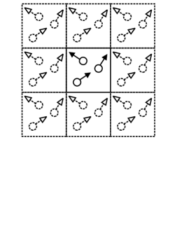
Figure 1: This picture depicts the idea of periodic boundary conditions. The box that is located in the center is the space of interest. We call this the ‘real box’.

In this work, we focus our investigation on the thermodynamic properties of a hadronic system. For this purpose, we consider a system in a cubic box and impose periodic boundary conditions in configuration space; i.e., if a particle leaves the box, another one with the same momentum enters from the opposite side. We display the boundary conditions pictorially in Fig. 1, where the box located in the center is the system we refer to as the ‘real box’ and the others are replicas. When we survey would-be collision points of the particles in the real box, we have to survey the collisions not only between particles in the real box but also with the particles in replicas.

The energy density $\varepsilon$ and the baryon number density $n_{B}$ in the box are fixed as input parameters, and these quantities are conserved throughout the simulation. The initial distributions of nucleons are given by uniform random distributions in phase space. The momenta of the particles are adjusted to satisfy the initial condition of energy, $\sum_{i=1}^{N}\sqrt{m^{2}_{i}+\mbox{\boldmath${p}$}^{2}_{i}}=\varepsilon\cdot V$, in the center-of mass system of the particles: $\sum_{i=1}^{N}\mbox{\boldmath${p}$}_{i}=\mbox{\boldmath${0}$}$. After setting the initial state in the above manner, time evolution as described by the event generator URASiMA takes place. Though the initial particles are only nucleons, many mesons are produced through interactions.

In order to confirm the realization of the stationarity of the system, we monitor particle densities and collision frequencies. We also check energy distributions of each particle. According to these methods of confirmation, as time increases, the system seems to become stationary. Whether the energy distributions approach the Boltzmann distribution is a fundamental question. If the system is in thermal equilibrium, the slope parameters of the energy distributions for all particles should converge to the same value, i.e., the inverse of temperature. In order to confirm this, we analyze the temporal evolution of the inverse slopes of various particles.

Running URASiMA many times with the same input parameters and taking the stationary configuration in equilibrium, we can obtain statistical ensembles with fixed temperature and fixed baryon number density. By using these ensembles, we can calculate thermodynamic quantities, such as the particle density, pressure, and so on, as functions of temperature and baryon number density.

2.2 Event generator URASiMA

URASiMA was originally designed to simulate ultra-relativistic AA collision experiments. (Here we call it URASiMA-A.)[20]  For this investigation, we improved URASiMA to study thermo-equilibrium systems in a box (URASiMA-B). In both models, collisions are realized when the distance between particles becomes smaller than their interaction range, which is defined by the relevant total cross-section. We describe the fully relativistic method to search for would-be collision points in Appendix A.1. The fundamental processes in the URASiMA-A/B are 2-body elastic and quasi-elastic collisions between hadrons, multi-particle productions, and strong decays of resonances. Hadronic experimental data are used as an input to the model.[29]  The processes which URASiMA-B includes are as follows:

$$NN\leftrightarrow NR,$$ (1)

$$NN\leftrightarrow\Delta_{1232}\Delta_{1232},$$ (2)

$$R\leftrightarrow N\pi,$$ (3)

$$R\leftrightarrow R^{\prime}\pi,$$ (4)

$$R\leftrightarrow Nr,$$ (5)

$$r\leftrightarrow\pi\pi,$$ (6)

$$NN\rightarrow NN+\;n\;\mbox{secondaries}\;(n\geq 3).$$ (7)

Here $R$ and $r$ denote baryon and meson resonances, respectively. The list of particles in URASiMA-B is given in Table 1. For the calculation of cross sections for quasi-2-body processes, we follow the work of Teis et al. [23]ref:Hub1  Cross sections of resonance absorptions such as $NR\rightarrow NN$ are calculated using the reciprocity of the S matrix. (See Appendix A.2.) [26]ref:Li1  A detailed explanation of multi-particle production is given in Appendix A.3.

Table 1: Baryons, mesons and their resonances included in URASiMA.

N	$N_{938}$	$N_{1440}$	$N_{1520}$	$N_{1535}$	$N_{1650}$	$N_{1675}$	$N_{1680}$	$N_{1720}$
$\Delta$	$\Delta_{1232}$	$\Delta_{1600}$	$\Delta_{1620}$	$\Delta_{1700}$	$\Delta_{1905}$	$\Delta_{1910}$	$\Delta_{1950}$
meson	$\pi$	$\sigma_{800}$	$\rho_{770}$

In the case of high-energy hadron/nuclear collisions, absorption processes are not so important. URASiMA-A includes direct multi-particle production ($n$ $\geq$ 1), and 1-$\pi$ production/absorption via $\Delta_{1232}$. In spite of the limited number of processes and particle species, URASiMA-A reproduces the global features of the experimental data quite well.[20]

However, in studies of thermo-equilibrium systems, whether detailed balance is maintained or not is an important property of the generator. Though the contributions of the multi-particle productions dominate the system at early stages of the non-equilibrated system, the reverse process plays an important role in the later, equilibration stage. The absence of reverse processes leads to one-way conversion of the energy to particles and an artificial temperature saturation in the equilibrated system.[13, 22]  However, the exact treatment of multi-particle absorption processes is very difficult. In order to treat them effectively with URASiMA-B, direct 1-$\pi$ and 2-$\pi$ productions are completely replaced by successive processes of quasi-elastic collisions and decays of resonances, and 1-$\pi$ and 2-$\pi$ absorptions through resonances are naturally included in the model. For this purpose, URASiMA-B contains $\Delta$ and $N^{*}$ particles whose masses are up to 2 GeV. We successfully reproduced 1-$\pi$, 2-$\pi$ and inelastic cross sections of $NN$ collisions up to $\sqrt{s}=$ 3 GeV without direct productions. This is the main difference between URASiMA-A and URASiMA-B. For $\sqrt{s}>3$ GeV, in order to obtain an appropriate total cross section, we need to take direct production processes into account. In our simulation, only at this point is detailed balance broken. Nevertheless, if the temperature is much smaller than 3 GeV, the influence of the breaking of detailed balance is negligibly small. For example, if the temperature of the system is 100 MeV, the occurrence of such a process is suppressed by a factor of exp($-30$), and thus the time scale to detect the violation of detailed balance is very much longer than the hadronic scale.

In order to demonstrate the descriptive ability of URASiMA-B, we compare its results with experimental data of the high energy nuclear collisions at BNL/AGS in Appendix A.4.

3 Results

3.1 Parameters

Table 2: Input parameters. Here $V$ is the volume of the box, $n_{B}$ is the baryon number density, and $\varepsilon$ is the total energy density.

$V$ [fm3]	$n_{B}$ [fm-3]	$\varepsilon$ [GeV/fm3]
$\;64.\;$	$\begin{array}[]{l}.156\\ .234\\ .313\end{array}$	$\begin{array}[]{l@{\s}l@{\s}l@{\s}l@{\s}l@{\s}l@{\s}l@{\s}l@{\s}l@{\s}l@{\s}l}.250\hfil\hskip 8.53581pt&.300\hfil\hskip 8.53581pt&.313\hfil\hskip 8.53581pt&.370\hfil\hskip 8.53581pt&.463\hfil\hskip 8.53581pt&.556\hfil\hskip 8.53581pt&.625\hfil\hskip 8.53581pt&.648\hfil\hskip 8.53581pt&.741\hfil\hskip 8.53581pt&.833\hfil\hskip 8.53581pt&.938\\ \hfil\hskip 8.53581pt&.300\hfil\hskip 8.53581pt&\hfil\hskip 8.53581pt&.370\hfil\hskip 8.53581pt&.463\hfil\hskip 8.53581pt&.556\hfil\hskip 8.53581pt&\hfil\hskip 8.53581pt&.648\hfil\hskip 8.53581pt&.741\hfil\hskip 8.53581pt&.833\hfil\hskip 8.53581pt&\\ \hfil\hskip 8.53581pt&\hfil\hskip 8.53581pt&\hfil\hskip 8.53581pt&.370\hfil\hskip 8.53581pt&.463\hfil\hskip 8.53581pt&.556\hfil\hskip 8.53581pt&\hfil\hskip 8.53581pt&.648\hfil\hskip 8.53581pt&.741\hfil\hskip 8.53581pt&.833\hfil\hskip 8.53581pt&\\ \end{array}$
$\;128.\;$	$\begin{array}[]{l}.156\\ .234\\ .313\end{array}$	$\begin{array}[]{l@{\s}l@{\s}l@{\s}l@{\s}l@{\s}l@{\s}l@{\s}l@{\s}l@{\s}l@{\s}l}.250\hfil\hskip 8.53581pt&.300\hfil\hskip 8.53581pt&\hfil\hskip 8.53581pt&.370\hfil\hskip 8.53581pt&.463\hfil\hskip 8.53581pt&.556\hfil\hskip 8.53581pt&\hfil\hskip 8.53581pt&.648\hfil\hskip 8.53581pt&.741\hfil\hskip 8.53581pt&.833\hfil\hskip 8.53581pt&\\ \hfil\hskip 8.53581pt&.300\hfil\hskip 8.53581pt&\hfil\hskip 8.53581pt&.370\hfil\hskip 8.53581pt&.463\hfil\hskip 8.53581pt&.556\hfil\hskip 8.53581pt&\hfil\hskip 8.53581pt&.648\hfil\hskip 8.53581pt&.741\hfil\hskip 8.53581pt&.833\hfil\hskip 8.53581pt&\\ \hfil\hskip 8.53581pt&\hfil\hskip 8.53581pt&\hfil\hskip 8.53581pt&.370\hfil\hskip 8.53581pt&.463\hfil\hskip 8.53581pt&.556\hfil\hskip 8.53581pt&\hfil\hskip 8.53581pt&.648\hfil\hskip 8.53581pt&.741\hfil\hskip 8.53581pt&.833\hfil\hskip 8.53581pt&\\ \end{array}$
$\;216.\;$	$\begin{array}[]{l}.157\\ .231\\ .315\end{array}$	$\begin{array}[]{l@{\s}l@{\s}l@{\s}l@{\s}l@{\s}l@{\s}l@{\s}l@{\s}l@{\s}l@{\s}l}\hfil\hskip 8.53581pt&\hfil\hskip 8.53581pt&\hfil\hskip 8.53581pt&.370\hfil\hskip 8.53581pt&.463\hfil\hskip 8.53581pt&.556\hfil\hskip 8.53581pt&\hfil\hskip 8.53581pt&.648\hfil\hskip 8.53581pt&.741\hfil\hskip 8.53581pt&.833\hfil\hskip 8.53581pt&\\ \hfil\hskip 8.53581pt&\hfil\hskip 8.53581pt&\hfil\hskip 8.53581pt&.370\hfil\hskip 8.53581pt&.463\hfil\hskip 8.53581pt&.556\hfil\hskip 8.53581pt&\hfil\hskip 8.53581pt&.648\hfil\hskip 8.53581pt&.741\hfil\hskip 8.53581pt&.833\hfil\hskip 8.53581pt&\\ \hfil\hskip 8.53581pt&\hfil\hskip 8.53581pt&\hfil\hskip 8.53581pt&.370\hfil\hskip 8.53581pt&.463\hfil\hskip 8.53581pt&.556\hfil\hskip 8.53581pt&\hfil\hskip 8.53581pt&.648\hfil\hskip 8.53581pt&.741\hfil\hskip 8.53581pt&.833\hfil\hskip 8.53581pt&\\ \end{array}$
$\;1000.\;$	$\begin{array}[]{l}.157\\ .231\\ .315\end{array}$	$\begin{array}[]{l@{\s}l@{\s}l@{\s}l@{\s}l@{\s}l@{\s}l@{\s}l@{\s}l@{\s}l@{\s}l}.250\hfil\hskip 8.53581pt&.300\hfil\hskip 8.53581pt&\hfil\hskip 8.53581pt&.370\hfil\hskip 8.53581pt&.463\hfil\hskip 8.53581pt&.556\hfil\hskip 8.53581pt&\hfil\hskip 8.53581pt&.648\hfil\hskip 8.53581pt&.741\hfil\hskip 8.53581pt&.833\hfil\hskip 8.53581pt&\\ \hfil\hskip 8.53581pt&.300\hfil\hskip 8.53581pt&\hfil\hskip 8.53581pt&.370\hfil\hskip 8.53581pt&.463\hfil\hskip 8.53581pt&.556\hfil\hskip 8.53581pt&\hfil\hskip 8.53581pt&.648\hfil\hskip 8.53581pt&.741\hfil\hskip 8.53581pt&.833\hfil\hskip 8.53581pt&\\ \hfil\hskip 8.53581pt&\hfil\hskip 8.53581pt&\hfil\hskip 8.53581pt&.370\hfil\hskip 8.53581pt&.463\hfil\hskip 8.53581pt&.556\hfil\hskip 8.53581pt&\hfil\hskip 8.53581pt&.648\hfil\hskip 8.53581pt&.741\hfil\hskip 8.53581pt&.833\hfil\hskip 8.53581pt&\\ \end{array}$

Focusing our interest on the region of temperature and baryon number density which is expected to be produced in high energy nuclear collisions, we used the input parameters given in Table 2. Here $n_{B}=0.156$ fm^-3 is taken as the baryon number density of normal nuclear matter. Thus, the baryon number density in our simulation corresponds to 1 – 2 times larger than that of normal nuclear matter. The total isospin of the system is set to zero, i.e., the number of protons is equal to the number of neutrons at the start.

In this paper we generated a statistical ensemble through two different methods, the phase average ($200$ event) and the long-time average ($1$ event). We compared the thermodynamic quantities obtained for the two ensembles in the case of $V=64.0$ fm³, and we confirmed that ergodicity holds to sufficient precision. In this paper, thermodynamic quantities are calculated from long-time averages, and the phase average is used when we study the time evolution of the system.

3.2 Chemical equilibration

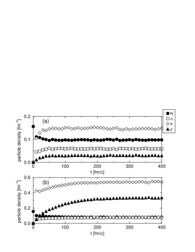
Figure 2: The time evolution of particle densities for each particle with $V=64.0$ fm³. Two results are shown, (a) that for $n_{B}=0.156$ fm^-3, $\varepsilon=0.313$ GeV/fm³, and (b) that for $n_{B}=0.156$ fm^-3, $\varepsilon=0.938$ GeV/fm³.

Figures 2 (a) and (b) display the time evolutions of particle densities. These figures show that the system approaches the stationary state with time. The saturation of particle densities indicates the realization of chemical equilibrium. In order to confirm the detailed balance of each reaction processes, we present time evolutions of collision frequencies for all kinds of reaction processes in Fig. 3. As seen them in the later stages, the collision frequency of the multi-particle production is less than $10^{-3}$ (fm/c)^-1, and the time scale of this process is much longer than that of other processes. Violation of reciprocity is important only for such long time-scale development. Actually, as shown in Fig. 4, no difference is observed in the time evolutions of particle densities when the multi-particle production is switched off after $t=150$ fm/c. Figure 5 shows that detailed balance actually holds on the time scale of several hundred fm/c. We conclude that chemical equilibrium in our system is realized.

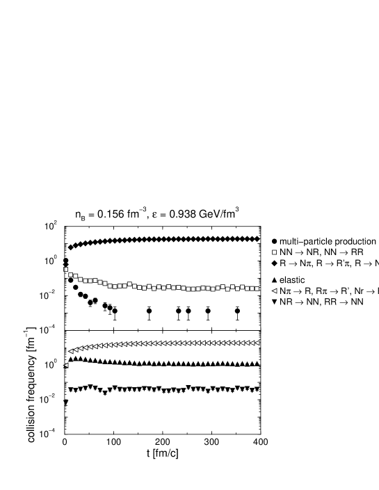
Figure 3: The time evolution of collision frequencies for various types of collisions: 2-body collisions and decays presented in Eqs. (1)–(6), multi-particle productions, and elastic collisions. Here $R$ denotes baryonic resonances, and $r$ denotes meson resonances. The calculation was done with $V=64.0$ fm³, $n_{B}=0.156$ fm^-3 and $\varepsilon=0.938$ GeV/fm³.

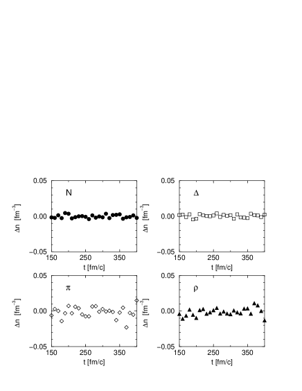
Figure 4: The difference between particle densities for the simulations with and without multi-particle production. The calculation without multi-particle production was realized by switching off the channel by hand at $t=150$ fm/c. The fact that the values in these figures are almost vanishing indicates that the contributions of the multi-particle productions are very small. The calculation was done with $V=64.0$ fm³, $n_{B}=0.156$ fm^-3 and $\varepsilon=0.938$ GeV/fm³.

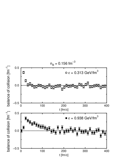
Figure 5: The time evolution of the balance of collision frequencies for two different energy densities, $\varepsilon=0.313$ GeV/fm³ and $\varepsilon=0.938$ GeV/fm³. In both calculations, the volume and baryon number density are $V=64.0$ fm³ and $n_{B}=0.156$ fm^-3. The vertical axes correspond to the difference between the frequencies of production processes and absorption processes. The fact that the quantities vanish for times greater than $t\sim 150$ fm/c indicates that the system satisfies detailed balance for $t\geq 150$ fm/c.

Here we briefly discuss the time scale of the chemical relaxation of the system. Figure 2 shows that the number density $n(t)$ seems to relax exponentially:

$$n(t) = (n_{B}-n(\infty))\cdot e^{-\frac{t}{\tau}}+n(\infty)\;\;\;\;\;\;\mbox{for}\;\;\;N,$$

$$n(t) = n(\infty)\cdot(1-e^{-\frac{t}{\tau}})\;\;\;\;\;\;\mbox{for}\;\;\;\Delta,\;\pi,\;\rho.$$ (8)

Based on this fact, we can easily estimate the relaxation time $\tau$ of particle densities that approach chemical equilibrium. We give the results for nucleon, pion and $\rho$ densities in Table 3. For the nucleon and pion, the obtained values of $\tau$ are in the range 7 – 20 fm/c, and they depend on the energy density. The values of $\tau$ obtained for $\rho$, however, are significantly larger.

Table 3: The relaxation time of particle densities for each particle with $n_{B}=0.156$ fm^-3.

$\varepsilon$ [GeV/fm3]	$N$ (=$\Delta$) [fm/c]	$\pi$ [fm/c]	$\rho$ [fm/c]
$0.313$	$7.1\pm 0.4$	$9.2\pm 0.3$	$21.2\pm 0.7$
$0.625$	$9.8\pm 0.5$	$13.3\pm 0.3$	$44.9\pm 1.0$
$0.938$	$10.6\pm 0.6$	$18.6\pm 0.4$	$68.5\pm 1.3$

Song and Koch calculated the chemical relaxation time of pions in hot hadron gas using the effective chiral Lagrangian.[34]  They estimated a chemical relaxation time for $\pi$ at $T\sim 150$ MeV as $10$ fm/c, which is close to the value obtained the present results. However, Table 3 shows the existence of several different time scales, and some of them are very long. Though these values may depend on the initial conditions of the simulation, our results indicate the possibility that hadronic systems have a long relaxation time in certain cases.

3.3 Thermal equilibration and temperature

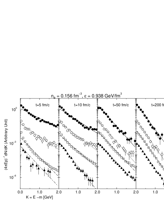
Figure 6: Energy distributions of $N_{938}$, $\Delta_{1232}$, $\pi$ and $\rho_{770}$ at four different values of time, $t=5$ fm/c, $t=10$ fm/c, $t=50$ fm/c and $t=200$ fm/c. The lines are the fitted results that are given by Boltzmann distributions, $C\exp(-\beta E)$. The calculation was done with $V=64.0$ fm³, $n_{B}=0.156$ fm^-3 and $\varepsilon=0.938$ GeV/fm³.

Figure 6 displays energy distributions of $N_{938},\Delta_{1232},\pi$ and $\rho_{770}$ at $t=5,\;10,\;50$ and $200$ fm/c. We plot the results as functions of the kinetic energy $K=E-m$, so that the horizontal axes for all particle species coincide. The energy distributions approach the Boltzmann distribution,

$$\frac{dN}{d^{3}\mbox{\boldmath${p}$}}=\frac{dN}{4\pi EpdE}=C\exp(-\beta E),$$ (9)

as time increases, where $\beta$ is the slope parameter of the distribution. Moreover, the slopes of the energy distributions converge to a common value. These results indicate that realization of thermal equilibrium.

Figure 7 (a) displays the time evolution of the quantities $\beta^{-1}$ that were calculated by fitting the energy distributions to a Boltzmann distribution. There, the dotted curves correspond to the time evolution of $\beta_{\pi}^{-1}$, i.e., the inverse slope of $\pi$. To confirm the establishment of the thermal equilibrium, the difference between the inverse slope and that of the pion at time $t$,

$$\Delta\beta_{j}^{-1}(t)=\beta_{j}^{-1}(t)-\beta_{\pi}^{-1}(t),$$ (10)

was calculated, where $j$ corresponds to $N_{938}$, $\Delta_{1232}$ and $\rho_{770}$. Figure 7 (b) shows the time evolution of these $\Delta\beta_{j}^{-1}$. From this figure, it is seen that the $\Delta\beta_{j}^{-1}$ become zero to within the accuracy of the statistics for times later than $150$ fm/c. Therefore, we conclude that thermal equilibrium is established at about $t=150$ fm/c; the values of the inverse slope parameters of the energy distribution for all particles become equal for later times. Thus we can regard this value as the temperature of the system. For later use, we define the temperature of the system as follows:

$$T(n_{B},\varepsilon)=\frac{\sum_{j}\beta_{j}^{-1}/\sigma_{j}^{2}}{\sum_{j}1/\sigma_{j}^{2}},\;\;\;\;\;\;j=N_{938},\Delta_{1232},\pi\;\;\mbox{and}\;\;\rho_{770},$$ (11)

where the $\beta_{j}^{-1}$ are calculated from energy distributions that are averaged over time after $t=200$ fm/c, and the $\sigma_{j}$ denote the errors of the $\beta_{j}^{-1}$.

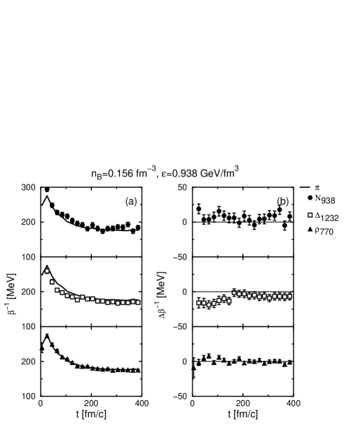
Figure 7: (a) The time evolution of the inverse slopes $\beta^{-1}$ for $N_{938}$, $\Delta_{1232}$, $\pi$ and $\rho_{770}$ with $V=64.0$ fm³, $n_{B}=0.156$ fm^-3, $\varepsilon=0.938$ GeV/fm³. The value of $\beta^{-1}$ was calculated from the fitting of energy distributions. Here the dotted curves represent the time evolution of $\beta^{-1}$ for $\pi$. (b) The time evolution of $\Delta\beta^{-1}$ for $N_{938}$, $\Delta_{1232}$ and $\rho_{770}$ with $V=64.0$ fm³, $n_{B}=0.156$ fm^-3, $\varepsilon=0.938$ GeV/fm³. Here $\Delta\beta^{-1}$ is defined in Eq. (10). The realization of thermal equilibrium can be concluded from these graphs.

3.4 Thermodynamic quantities

Figures 8–10 show the relations between the temperature and thermodynamic quantities such as energy density, $\varepsilon=\frac{1}{V}\sum_{i=1}^{\mbox{\scriptsize all particles}}E_{i}$, particle density, and pressure, $P=\frac{1}{3V}\sum_{i=1}^{\mbox{\scriptsize all particles}}\frac{\mbox{\boldmath${p}$}_{i}\cdot\mbox{\boldmath${p}$}_{i}}{E_{i}}$. In these figures, all curves correspond to the relativistic Fermi-Dirac or Bose-Einstein gas with a finite mass width; i.e., eq:eoset ε(T,μ) & = ∑_h d_h∫∫dmd3p(2π)3 ρR(m) EeE-μT±1,
eq:eospt n(T,μ) = ∑_h d_h∫∫dm d3p(2π)3 ρR(m)eE-μT±1,
eq:eosprt P(T,μ) = ∑_h d_h∫∫dm d3p(2π)3 p23E ρR(m)eE-μT±1, where $d_{h}$ is a degeneracy factor and $\rho_{R}(m)$ is the mass spectral function, which is given by the Breit-Wigner distribution for the resonances. In these calculation, the baryon chemical potential $\mu_{B}$ is adjusted to reproduce the total baryon number density, whereas the meson chemical potential $\mu_{m}$ is fixed to zero.

In Eq. (3.4), anti-baryons are ignored, because our event generator does not contain anti-baryons. However, their contributions to thermodynamic quantities are negligible if the temperature is below 170 MeV, since the ratio of the anti-baryon number to the baryon number is suppressed by $e^{-\frac{2\mu_{B}}{T}}$. Even at the smallest value of the chemical potential, $\mu_{B}=250$ MeV ($n_{B}=0.157$ fm^-3, $T=170$ MeV), the factor is about 5% at most. Therefore, quantitative error caused by ignoring anti-baryons should be only about several percent.

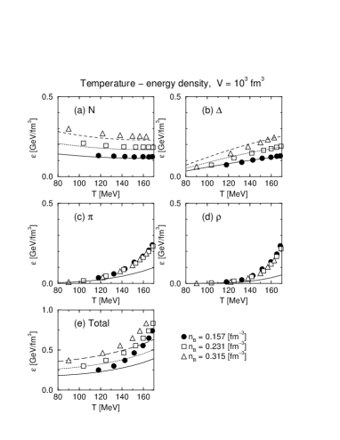
Figure 8: The equation of state of a mixed hadron gas at finite temperature ($80$ MeV $<T<170$ MeV) and finite baryon density ($0.157$ fm${}^{-3}<n_{B}<0.315$ fm^-3). The energy densities of (a) $N$, (b) $\Delta$ (the sum of all resonances), (c) $\pi$, (d) $\rho_{770}$ and (e) total are plotted as functions of the temperature. The curves correspond to the free gas model represented by Eq. (LABEL:eq:eoset).

Figures 8–10 (a) and (b) display the equations of state of baryons. In these figures, it is difficult to see the difference between our results and those for the calculation of the free gas model. This is the result for the when it is under the strict constraint of baryon number conservation, which fixes the total number densities of the $N$ and $\Delta$ particles. Thus a close look at the fractions of baryon resonances is necessary in order to recognize the difference between our model and free gas model.

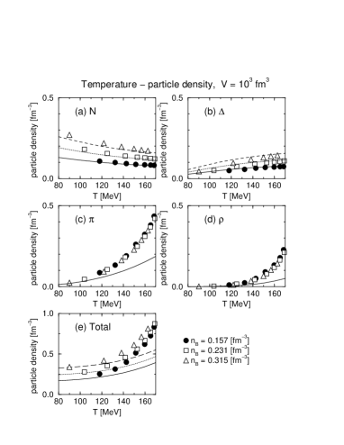
Figure 9: Particle densities of (a) $N$, (b) $\Delta$ (the sum of all resonances), (c) $\pi$, (d) $\rho_{770}$ and (e) total are plotted as functions of the temperature. The curves correspond to the free gas model represented by Eq. (LABEL:eq:eospt).

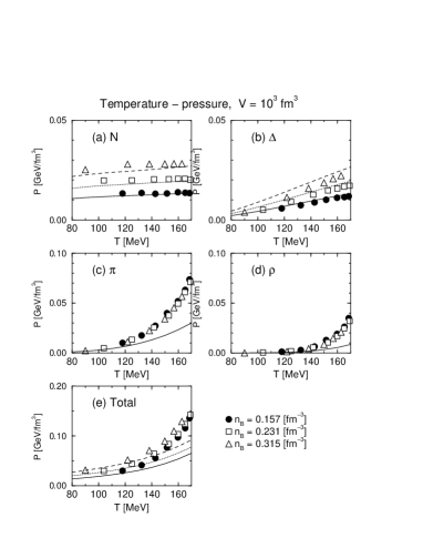
Figure 10: Pressures of (a) $N$, (b) $\Delta$ (the sum of all resonances), (c) $\pi$, (d) $\rho_{770}$ and (e) total are plotted as functions of the temperature. The curves correspond to the free gas model represented by Eq. (LABEL:eq:eosprt).

Figure 11 displays the particle ratios of $N_{938}$, $\Delta_{1232}$ and other heavy resonances, $N^{*}$ and $\Delta^{*}$. At lower temperature ($T=125$ MeV), the difference between our results and those of the free gas calculations is small. However, at higher temperature ($T>150$ MeV), the ratios of light baryons ($N_{938}$ and $\Delta_{1232}$) become smaller, and those of heavy resonances, conversely, become larger. Thus we find that the influence of interactions clearly appears above $T\sim m_{\pi}$. Such an enhancement of heavy baryons grows as the temperature increases. The maximum value of the enhancement reaches 12–15% near $T=170$ MeV.

Figures 8–10 (c) and (d) display the equations of state of mesons. As in the case of baryons, the deviation from the free gas model appears at temperatures above

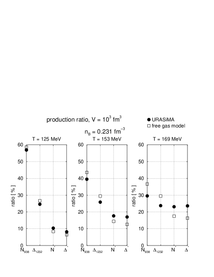
Figure 11: The production ratio of $N_{938}$, $\Delta_{1232}$ and other heavy resonances, $N^{*}$ and $\Delta^{*}$. Calculations were done with $n_{B}=0.231$ fm^-3 and temperatures $T=125$ MeV, $153$ MeV, $169$ MeV, respectively.

$T\sim m_{\pi}$. Above this temperature, meson production is large, and the increase of the temperature becomes moderate.

In a previous study,[13]  the saturation of the temperature appeared, and there we called it the “Hagedorn-like limiting temperature.” However, it was an artificial saturation of the temperature, because of the luck of the reversal process of multi-particle production. In the calculation of the improved URASiMA, this limiting temperature does not appear, and we believe that this is an important result of taking detailed balance into account.

Moreover, our results indicate that the equations of state of baryons and mesons are closely related through meson-baryon interactions, such as $\pi N\rightarrow R$ and their inverse processes. The enhancement of heavy baryon resonances causes the increase in the abundances of mesons, and vice versa. Heavy resonances readily produce 2$\pi$, and thus the enhancement of heavy baryon resonances promotes meson production. Therefore, interactions between mesons and baryons are very important in the study of the properties of a mixed hadron gas.

3.5 Entropy

Figure 12 plots the entropy per baryon versus the temperature. Here the curves correspond to free gas calculations. In order to define the entropy, we divide the phase space into small cells whose volumes are equal to $(\hbar c)^{3}$fm³(GeV/c)³. We distinguish each cell by the index $l$. The density operator of a cell $\rho_{l}=\rho(\mbox{\boldmath${x}$}^{l},\mbox{\boldmath${p}$}^{l})$ is defined as follows:

$$\rho_{l}=\left\{\begin{array}[]{ll}1:&\mbox{Particle exists in the {\it l}-th cell.}\\ 0:&\mbox{The {\it l}-th cell is empty.}\end{array}\right.$$ (12)

The definition of the entropy is given by

$$S = -\mbox{Tr}\left\{\langle\rho_{l}\rangle\ln\langle\rho_{l}\rangle\right\},$$ (13)

$$= -\sum_{l}^{\mbox{\scriptsize all cells in phase space}}\langle\rho_{l}\rangle\ln\langle\rho_{l}\rangle,$$

where $\langle\rho_{l}\rangle$ is the ensemble average of the density operator of a cell,

$$\langle\rho_{l}\rangle=\frac{1}{\mbox{number of ensemble states}}\sum_{\mbox{{\scriptsize ensemble}}}\rho_{l},$$ (14)

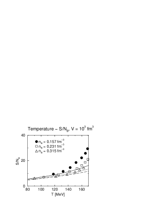
Figure 12: The entropy per baryon plotted as a function of the temperature. The curves correspond to the free gas model.

and the trace constitutes the average over phase space. Figure 12 shows that the hadron gas has a larger value of $S/N_{B}$ in the present model than in the free gas model for $T>m_{\pi}$, because a large part of the energy of the system goes into particle (entropy) production. Moreover, our results show a clear dependence on the baryon density. Thus, the frequently assumed ansatz that $S/N_{B}$ is insensitive to $n_{B}$ seems unreasonable. Therefore, our results indicate that the free gas model provides a poor description for these quantities above $T=m_{\pi}$. Hence, we should be more careful in using a free gas model in the interpretation of ultra-relativistic heavy ion experiments, even if some corrections, such as the excluded volume effect, are considered.[35]ref:Mun3

Furthermore, some models seem insufficient in counting the dynamical degrees of freedom per baryon. For example, EOS based on the $\sigma$-$\omega$ model[38] predicts $S/N_{B}\sim 5$ (see Ref. ref:Rei1) independently of the temperature, while our result gives $S/N_{B}\sim 18.6\pm 0.2$ at $T=150$ MeV and $29.2\pm 0.1$ at $T=170$ MeV for the normal nuclear matter density.

3.6 Energy density dependence of the pressure

From Fig. 13 (a), we find that our results and those of the free gas calculations exhibit almost a linear dependence of the pressure on the energy density within the range of the present study. Our results can be fitted by the following function with parameters $b$ and $\varepsilon_{0}$:

$$P(\varepsilon)=b\cdot(\varepsilon-\varepsilon_{0}).$$ (15)

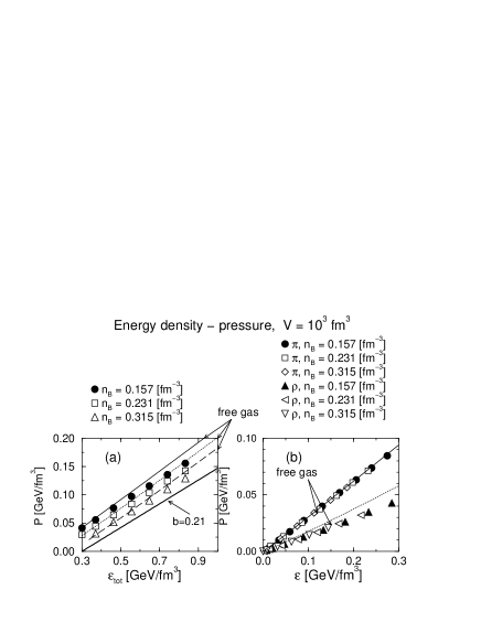
Figure 13: (a) Pressures are plotted as functions of the energy density. Free gas results and a line with slope 0.21 are also shown. (b) Partial pressures of mesons as functions of their partial energy densities.

The values of these parameters at three different baryon number densities are shown in Table 4.

To clarify the situation further, we now investigate partial pressures. As shown in Figs. 8–10, pressures and energy densities of baryons as functions of the temperature do not deviate from their forms for the free gas. Contrastingly, the partial pressure of the mesons shows a clear deviation from that of the free gas model. In Fig. 13 (b) the partial pressures of mesons are plotted as functions of the corresponding partial energy densities. It is interesting that pions behave like a free gas with regard to this quantity. On the other hand, the slope of the $\rho$ meson is smaller in the present case than in the free gas. This result indicates that the $\rho$ meson and its interactions play an important role in determining the thermodynamic properties of a hadron gas.

Table 4: Fitting parameters for Fig. 13.

$n_{B}$ [fm-3]	$b$	$\varepsilon_{0}$ [GeV/fm3]
$0.157$	$0.2171\pm 0.0009$	$0.1163\pm 0.0026$
$0.231$	$0.2122\pm 0.0008$	$0.1633\pm 0.0023$
$0.315$	$0.2083\pm 0.0007$	$0.2188\pm 0.0021$

3.7 Finite size effect

Finally, we check the finite size effect of our calculation. To see this, we prepared four different sizes of the boxes, $64.0$ fm³, $128.0$ fm³, $216.0$ fm³ and $1000.0$ fm³. The volume dependence of the total particle density is shown in Fig. 14. We were not able to find any differences among the four sizes of the box. Other thermodynamic quantities yield the same result. As concerns thermodynamic quantities, we can regard $64.0$ fm³ as a sufficiently large spatial size.

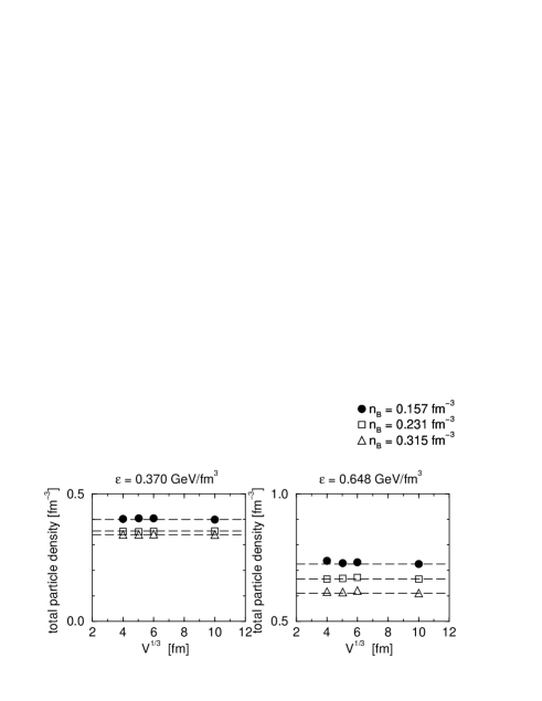
Figure 14: Volume dependence of the total particle density for $\varepsilon=0.370$, $0.648$ GeV/fm³.

We also compared relaxation lengths for various spatial box sizes. In a previous paper, we investigated the baryon diffusion constant.[14]  First, the fluctuation-dissipation theorem tells us that diffusion constant $D$ is given by the current (velocity) correlation,[40]

$$D=\frac{1}{3}\int_{0}^{\infty}\langle\mbox{\boldmath${v}$}(t)\cdot\mbox{\boldmath${v}$}(t+t^{\prime})\rangle dt^{\prime}.$$ (16)

In our definition, the correlation function $\langle\cdots\rangle$ is given by

$$\langle\cdots\rangle=\frac{1}{\mbox{number of ensemble states}}\sum_{\mbox{{\scriptsize ensemble}}}\frac{1}{\mbox{number of baryons}}\sum_{\mbox{{\scriptsize baryons}}}\cdots.$$ (17)

The correlation functions are damped exponentially with time (see Fig. 15):

$$\langle\mbox{\boldmath${v}$}(t)\cdot\mbox{\boldmath${v}$}(t+t^{\prime})\rangle\propto\exp{\left(-\frac{t^{\prime}}{\tau_{B}}\right)}.$$ (18)

Thus the diffusion constant can be rewritten in the simple form

$$D=\frac{1}{3}\langle\mbox{\boldmath${v}$}(t)\cdot\mbox{\boldmath${v}$}(t)\rangle\tau_{B},$$ (19)

where $\tau_{B}$ is the relaxation time of the baryon current. Figure 16 shows the volume dependence of $\tau_{B}\cdot\langle v_{B}\rangle$, where $\langle v_{B}\rangle$ denotes the average speed of baryons, and thus $\tau_{B}\cdot\langle v_{B}\rangle$ has dimensions of length. Though this quantity has a clear dependence on the size of the box at low energy density ($\varepsilon=0.370$ GeV/fm³), this box size dependence seems to disappear for volumes larger than about $6^{3}$ fm³. In this work, to be safe, we used a box of volume $V=1000$ fm³. Therefore, the result in this paper can be considered free of any box-size effect.

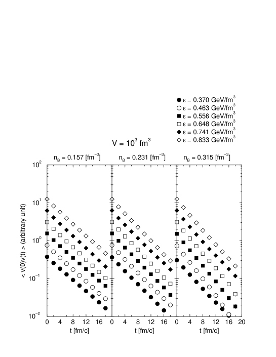
Figure 15: Velocity correlation of the baryons as a function of time. The normalization of the data is arbitrary.

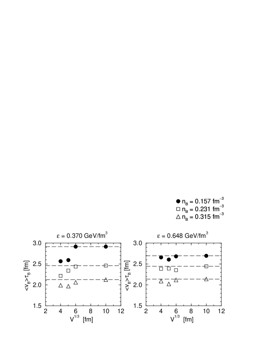
Figure 16: The relaxation time multiplied by average velocity as a function of the volume of the system.

4 Summary

In this paper, we studied the equilibration and the equation of state of hot ($80$ MeV $<T<170$ MeV) hadron gas with finite baryon number density ($0.157$ fm^-3 $<n_{B}<0.315$ fm^-3) by using the event generator URASiMA, which maintains detailed balance in the practical sense in the hadronic energy scale. We performed molecular dynamical calculations for a system of hadrons in a box with periodic boundary conditions. The energy density and baryon number in our simulation correspond to those of a hot hadron fluid, which is believed to be produced in high energy nuclear collisions. Our results for thermodynamic quantities can be related to experimental data through statistical models and hydrodynamic models.[16]

Collision frequencies and particle densities exhibit saturation as the time evolution proceeds. These results indicate that the system reaches chemical equilibration. We also studied the thermal equilibration of the system from the time evolution of the inverse slopes of the energy distributions. To confirm that thermal equilibrium is established, it was demonstrated that the slope parameters of $N_{938}$, $\Delta_{1232}$, $\pi$ and $\rho_{770}$ become almost identical for times greater than $t\sim 150$ fm/c. Thus the temperature of the system can be defined after this time.

After the equilibration, thermodynamic quantities were evaluated, and the equation of state was investigated. Energy densities, number densities, pressures and entropies per baryon were plotted as functions of the temperature. Deviations from the free gas model were manifestly observed above $T\sim m_{\pi}$. Above this temperature, the excitation of heavy baryon resonances were found to be enhanced, and meson production was found to be significant. Those effects suppress the increase of the temperature, but the saturation of the temperature, as in the case of Hagedorn’s limiting temperature, never occurs. These notable differences from previous works[22, 13] are important results of the proper maintenance detailed balance between production processes and absorption processes. For a reliable simulation of a statistical system, detailed balance is essentially important. In our study, we found large values of the entropy per baryon. This depends strongly on the baryon density above $T\sim m_{\pi}$. The pressures exhibit linear dependences on the energy densities within the range of present study. Such behavior was analyzed in detail by looking at relations between partial pressures and partial energy densities of mesons. We find that the $\rho$ meson and its interactions play an important role in the thermodynamic properties of the hadron gas.

Because the temperature in this investigation (80–170 MeV) is much lower than the mass of a $K\bar{K}$ pair, the hadron gas is mainly composed of non-strange particles. For this reason, strange particles are not considered in our model. However, in the early stages of the AA collision, the energy density can be very high, and the strangeness degree of freedom should play an important role. Including strange particles in our model is the next task, and we are now in process of doing so.

The investigation reported in this paper was focused on “hadronic scale” energy densities and baryon number densities. However, it would be interesting to perform calculations at higher energy densities and baryon number densities. Our EOS without a phase transition can work as a helpful reference to the equation of state with a QGP phase transition.

Appendix A Event Generator URASiMA

A.1 The search for would-be collision points

After a collision at the space-time point $x_{0\,i}^{\mu}=(t_{0\,i},\mbox{\boldmath${x}$}_{0\,i})$, the trajectory of the $i$-th particle is given by the straight line

$$x_{i}^{\mu}=(t_{i},\mbox{\boldmath${x}$}_{i})=\frac{p_{i}^{\mu}}{m_{i}}\xi_{i}+x_{0\,i}^{\mu},$$ (20)

where $p_{i}^{\mu}=(E_{i},\mbox{\boldmath${p}$}_{i})$ and $m_{i}$ are the momentum and the mass of the particle after the collision, and $\xi_{i}$ represents the proper time:

$$\xi_{i}\equiv\frac{m_{i}}{E_{i}}(t_{i}-t_{0\,i}).$$ (21)

Figure 17: The condition for which the collision occurs in the CM frame of two particles. In this frame, the momentum vector $p^{*}_{1}$ $\|$ $p^{*}_{2}$ and the difference between positions $x^{*}_{1}(t^{*}_{1})-x^{*}_{2}(t^{*}_{2})$ become perpendicular at the point of nearest approach. In this situation, a collision occurs if Eq. (22) is satisfied.

Equation (20) holds until the next interaction occurs.

We adopt a hard sphere approximation for binary collisions; that is, a collision occurs whenever the condition

$$\pi\mbox{\boldmath${b}$}^{*\,2}<\sigma$$ (22)

is satisfied, where $|\mbox{\boldmath${b}$}^{*}|$ is the impact parameter in the CM frame of two particles, and $\sigma$ is the total cross section. For the manifestly relativistic formulation, it is important to express the collision condition (22) in a covariant way. For this purpose, we consider the CM frame of two particles, 1 and 2 (see Fig. 17). When two particles are at the points of their closest approach, the impact parameter $\mbox{\boldmath${b}$}^{*}\equiv\mbox{\boldmath${x}$}^{*}_{1}(t^{*}_{1})-\mbox{\boldmath${x}$}^{*}_{2}(t^{*}_{2})$ and the time $t^{*}_{c}$ are defined as

$$(\mbox{\boldmath${x}$}^{*}_{1}(t^{*}_{1})-\mbox{\boldmath${x}$}^{*}_{2}(t^{*}_{2}))\cdot\mbox{\boldmath${p}$}^{*}_{j} = 0,\;\;\;\;\;\;(j=1,2)$$

$$t^{*}_{1}=t^{*}_{2}\equiv t^{*}_{c},$$ (23)

where $t^{*}_{c}$ denotes the time at which a collision may occur. Here, we define the total momentum $Q^{\mu*}$ and the difference of momenta $K^{\mu*}$ as

$$Q^{\mu*} \equiv p_{1}^{\mu*}+p_{2}^{\mu*}=(E_{1}^{*}+E_{2}^{*},0),$$

$$K^{\mu*} \equiv p_{1}^{\mu*}-p_{2}^{\mu*}=(E_{1}^{*}-E_{2}^{*},\mbox{\boldmath${p}$}^{*}_{1}-\mbox{\boldmath${p}$}^{*}_{2}).$$ (24)

Using $Q^{\mu*}$ and $K^{\mu*}$, Eq. (23) can be rewritten as

$$(\mbox{\boldmath${x}$}^{*}_{1}(t^{*}_{1})-\mbox{\boldmath${x}$}^{*}_{2}(t^{*}_{2}))\cdot\mbox{\boldmath${K}$}^{*} = 0,$$

$$(t^{*}_{1}-t^{*}_{2})Q^{0*} = 0.$$ (25)

The invariant expressions of Eq. (25) are easily obtained as follows:

$$(x_{1}-x_{2})\cdot Q = 0,$$

$$(x_{1}-x_{2})\cdot K = 0.$$ (26)

Replacing $x_{1}$ and $x_{2}$ in Eq. (26) by their forms in Eq. (20), we find the equations

$$\frac{p_{1}\cdot Q}{m_{1}}\xi_{1}-\frac{p_{2}\cdot Q}{m_{2}}\xi_{2}+X_{0}\cdot Q = 0,$$

$$\frac{p_{1}\cdot K}{m_{1}}\xi_{1}-\frac{p_{2}\cdot K}{m_{2}}\xi_{2}+X_{0}\cdot K = 0,$$ (27)

where $X^{\mu}_{0}=x^{\mu}_{0\,1}-x^{\mu}_{0\,2}$. The solutions of these equations are easily obtained as

$$\left(\begin{array}[]{c}\xi_{1}\\ \xi_{2}\end{array}\right)=\frac{-1}{J}\left(\begin{array}[]{cc}-\frac{p_{2}\cdot K}{m_{2}}&\frac{p_{2}\cdot Q}{m_{2}}\\ -\frac{p_{1}\cdot K}{m_{1}}&\frac{p_{1}\cdot Q}{m_{1}}\end{array}\right)\left(\begin{array}[]{c}X_{0}\cdot Q\\ X_{0}\cdot K\\ \end{array}\right),$$ (28)

where $J$ is defined as

$$J \equiv -\frac{(p_{1}\cdot Q)(p_{2}\cdot K)-(p_{1}\cdot K)(p_{2}\cdot Q)}{m_{1}m_{2}},$$ (29)

$$= -2\frac{(p_{1}\cdot p_{2})^{2}-(m_{1}m_{2})^{2}}{m_{1}m_{2}}.$$

Using Eqs. (20) and (28), the invariant expression for the impact parameter is given by

$$b^{2} \equiv (x_{1}-x_{2})^{2}$$ (30)

$$= X^{2}_{0}-\frac{(X_{0}\cdot Q)^{2}}{Q^{2}}-\frac{[(X_{0}\cdot K)-\frac{(K\cdot Q)(X_{0}\cdot Q)}{Q^{2}}]^{2}}{(K-\frac{(K\cdot Q)}{Q^{2}}Q)^{2}}.$$

This expression enables us to specify the collision point in terms of momenta and space-time coordinates of the starting points (the previous collision points). In the simulation, all candidates for collision are searched for using Eq. (30), and the earliest collision in the rest frame of the box is generated.

A.2 Absorption cross sections

By using the reciprocity of the S matrix, the absorption cross section can be related to the production cross section

$$\sigma_{N^{\prime\prime}R\rightarrow NN^{\prime}}=\frac{2}{g_{R}}\frac{1}{1+\delta_{NN^{\prime}}}\frac{p_{f}^{2}}{p_{i}^{2}}\sigma_{NN^{\prime}\rightarrow N^{\prime\prime}R},$$ (31)

with $\delta_{NN^{\prime}}$ the Kronecker $\delta$, which is equal to 1 when the final state nucleons belong to the same state. The relation Eq. (31) is limited to particles with definite masses. Extension of Eq. (31) to take into account the width of resonance mass is straightforward, [26]ref:Li1  and we have

$$\sigma_{N^{\prime\prime}R\rightarrow NN^{\prime}}=\frac{2}{g_{R}}\frac{m_{R}p^{2}_{f}}{1+\delta_{NN^{\prime}}}\frac{\sigma_{NN^{\prime}\rightarrow N^{\prime\prime}R}}{p_{i}\int^{\sqrt{s}-m_{N}}_{m_{\pi}+m_{N}}\frac{dm^{{}^{\prime}}_{R}}{2\pi}m^{{}^{\prime}}_{R}\rho_{R}(m^{{}^{\prime}}_{R})p^{{}^{\prime}}_{i}},$$ (32)

where $\rho_{R}(m^{{}^{\prime}}_{R})$ is the mass distribution function, which is given by the Breit-Wigner distribution.

A.3 Multi-particle productions

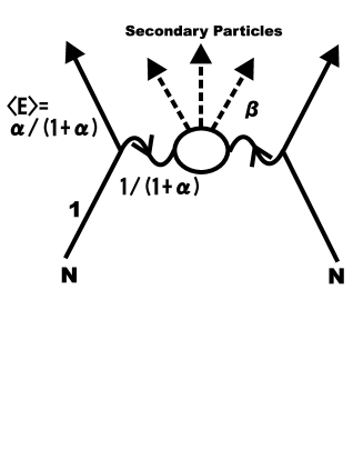
Figure 18: The diagram of the multi-particle production process for an $N+N$ inelastic collision. Here $\langle E\rangle$ denotes the average of the energy fraction that the primary nucleon carries after the collision. This quantity is related to the value of $\alpha$, which is one of the adjustable parameters. The remainder of the energy fraction is consumed by the production of secondary particles, whose momenta are determined according to the distribution characterized by $\beta$.

In high energy hadron-hadron collisions, n-particle ($n\geq 3)$ productions may occur. In our model, such multi-particle productions are treated as direct processes. Such processes are very important in the early stages, where energetic particles dominate the system. In the present simulation, initial states include many energetic nucleons, and multi-particle production takes place frequently. In the later stages, however, they seldom occur, and their effect is negligibly small.

In URASiMA, a multi-particle production process is realized by use of the multi-chain model,[17]ref:Kan1  where the exchange of a hadronic chain causes the direct emission of multipions. Figure 18 displays a diagram of $N+N$ inelastic collisions. In this figure, nucleons exchange a chain, which produces secondary particles. Such multi-particle production is specified by parameters as follows. The probability distribution of a light-like longitudinal momentum fraction $x_{N}$ that is carried by nucleons after collisions is given by

$$P(x_{N})=\alpha\cdot x^{\alpha-1}_{N}.$$ (33)

Table 5: Parameters of multi-particle production.

$\;\;\;\;\;\;\alpha\;\;\;\;\;\;$	$\;\;\;\;\;\;\beta\;\;\;\;\;\;$	$\;\;\;\;\;\;\tau_{0}$ [fm/c]
1	1.0	1.0

The average energy that is carried by nucleons is $\alpha/(\alpha+1)$ times the initial energy. The remainder, which is on average equal to $1/(\alpha+1)$, is consumed by the production of secondary particles.

In the C.M. frame of produced particles, the longitudinal momentum of the secondary particle behaves according to the distribution

$$\frac{dN}{dy}\propto\left(1-\frac{2m_{T}\cosh{y}}{\sqrt{\hat{s}}}\right)^{\beta},$$ (34)

with $m_{T}$ and $y$ the transverse mass and the rapidity of the secondary particle. The quantity $\sqrt{\hat{s}}$ stands for the energy deposited in the blob of the diagram.

Transverse momentum distributions of primary and secondary particles are given by gamma distributions:

$$\frac{dN_{j}}{dp_{T}}\propto p_{T}e^{-B_{j}\cdot p_{T}}.\;\;\;\;\;(j=\mbox{nucleon},\;\;\pi,\;\;\mbox{etc}.)$$ (35)

Here $p_{T}$ denotes the transverse momentum, and the slope parameter $B_{j}$ is another parameter of the model.

Secondary particles propagate freely without any interaction during the formation time $\tau$ after the emission,

$$\tau=\gamma\cdot\tau_{0}=\frac{E}{m}\cdot\tau_{0},$$ (36)

where the proper formation time $\tau_{0}$ is also one of the parameters of URASiMA. Values of the parameters $\alpha$, $\beta$ and $\tau_{0}$ are listed in Table 5.

A.4 Comparisons with data of nucleus-nucleus collisions at high energies

In order to examine the descriptive power of the event generator URASiMA-B, we made comparisons with the data of high-energy nuclear collision experiments. In this case, the initial state is given by the energetic nucleons forming the nuclei in free space. All parameters of the model are tuned to reproduce the data of hadron-hadron collisions.[29]ref:Zab1

The results of our simulations are compared with the experimental data of the E802 collaboration for the Si + Al central collision at $14.6$ GeV/nucleon.[33]  Figure 19 displays the rapidity distributions for the proton (left) and $\pi^{+}$ (right), where the squares denote the results of our simulation and the filled circles denote the experimental results. Figure 20 shows the rapidity dependence of the inverse slopes of transverse momentum distributions for the proton (left) and $\pi^{+}$ (right). In both figures, URASiMA-B reproduces global features of experimental data quite well.

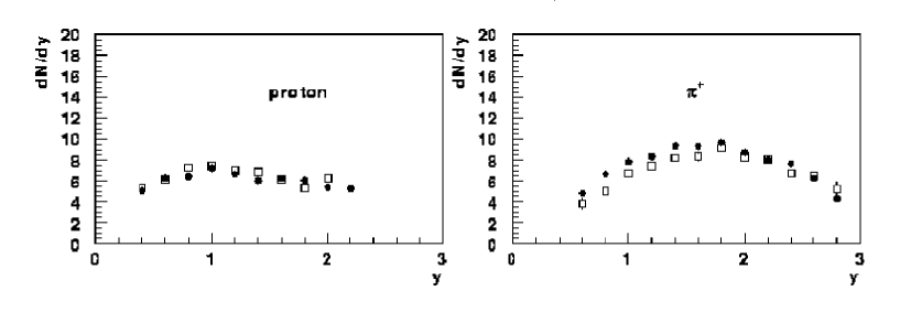
Figure 19: A comparison between experimental results and our simulations. We plot the rapidity distributions of the proton (left) and $\pi$ (right) for Si + Al central collisions at 14.6 GeV/nucleon obtained in the E802 collaboration. Here, the squares denote the results of our simulation, and the filled circles denote the experimental results.

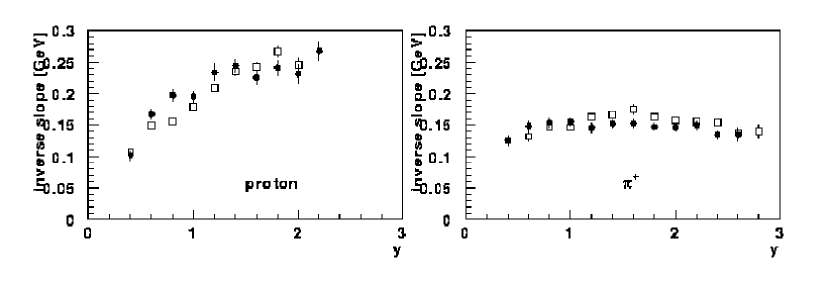
Figure 20: A comparison between experimental results and our simulations. We plot inverse slopes of transverse momentum distributions of the proton (left) and $\pi$ (right) for Si + Al central collisions at 14.6 GeV/nucleon obtained in the E802 collaboration. Here, the squares denote the results of our simulation, and the filled circles denote the experimental results.

References

- [1] For example, see the Proceedings of Quark Matter ’99, Nucl. Phys. A 661 (1999), 3c.
- [2] T. Kajino, Phys. Rev. Lett. 66 (1991), 125.
- [3] F. Karsch, E. Laermann and A. Peikert, Phys. Lett. B 478 (2000), 447.
- [4] M. Okamoto, A. Ali Khan, S. Aoki, R. Burkhalter, S. Ejiri, M. Fukugita, S. Hashimoto, N. Ishizuka, Y. Iwasaki, K. Kanaya, T. Kaneko, Y. Kuramashi, T. Manke, K. Nagai, M. Okawa, A. Ukawa and T. Yoshie, Phys. Rev. D 60 (1999), 4510.
- [5] G. Boyd, J. Engels, F. Karsch, E. Laermann, C. Legeland, M. Lütgemeier and B. Petersson, Nucl. Phys. B 469 (1996), 419.
- [6] I. M. Barbour, Nucl. Phys. A 642 (1998), 251.
- [7] O. Kaczmarek, J. Engels, F. Karsch and E. Laermann, in Proceedings of 17th International Symposium on Lattice Field Theory (LATTICE 99), Nucl. Phys. B Proc. Suppl. 83 (2000), 369.
- [8] S. Sakai, A. Nakamura and T. Saito, Nucl. Phys. A 638 (1998), 535c.
- [9] R. Hagedorn, cern-th-7190-94 (1994).
- [10] M. I. Gorenstein, A. P. Kostyuk and Ya. D. Krivenko, J. of Phys. G 25 (1999), 75.
- [11] C. P. Singh, B. K. Patra and K. K. Singh, Phys. Lett. B 387 (1996), 680.
- [12] H. Kouno and F. Takagi, Z. Phys. C 45 (1989), 43.
- [13] N. Sasaki and O. Miyamura, Prog. Theor. Phys. Suppl. No. 129 (1997), 39.
-
[14]
N. Sasaki, O. Miyamura, S. Muroya and C. Nonaka,
Phys. Rev. C 62 (2000), 1901.
N. Sasaki, O. Miyamura, S. Muroya and C. Nonaka, Europhys. Lett. 54 (2001), 38. - [15] N. Sasaki, O. Miyamura, S. Muroya and C. Nonaka, in preparation.
- [16] C. Nonaka, E. Honda and S. Muroya, Eur. Phys. J. C 17 (2000), 663.
- [17] A. Capella and A. Krzywicki, Phys. Rev. D 18 (1978), 3357.
- [18] K. Kinoshita, A. Minaka and H. Sumiyoshi, Prog. Theor. Phys. 61 (1979), 165.
- [19] T. Kanki, K. Kinoshita, H. Sumiyoshi and F. Takagi, Prog. Theor. Phys. Suppl. No. 97A (1988); T. Kanki, K. Kinoshita, H. Sumiyoshi and F. Takagi, Prog. Theor. Phys. Suppl. No. 97B (1989).
- [20] S. Daté, K. Kumagai, O. Miyamura, H. Sumiyoshi and X. Z. Zhang, J. Phys. Soc. Jpn. 64 (1995), 766.
- [21] S. A. Bass, M. Belkacem, M. Bleicher, M. Brandstetter, L. Bravina, C. Ernst, L. Gerland, M. Hofmann, S. Hofmann, J. Konopka, G. Mao, L. Neise, S. Soff, C. Spieles, H. Weber, L. A. Winckelmann, H. Stöcker, W. Greiner, C. Hartnack, J. Aichelin and N. Amelin, Prog. Part. Nucl. Phys. 41 (1998), 225.
- [22] M. Belkacem, M. Brandstetter, S. A. Bass, M. Bleicher, L. Bravina, M. I. Gorenstein, J. Konopka, L. Neise, C. Spieles, S. Soff, H. Weber, H. Stöcker and W. Greiner, Phys. Rev. C 58 (1998), 1727.
- [23] S. Teis, W. Cassing, M. Effenberger, A. Hombach, U. Mosel and Gy. Wolf, Z. Phys. A 356 (1997), 421.
- [24] V. Dmitriev, O. Sushkov and C. Gaarde, Nucl. Phys. A 459 (1986), 503.
- [25] S. Huber and J. Aichelin, Nucl. Phys. A 573 (1994), 587.
- [26] P. Danielewicz and G. F. Bertsch, Nucl. Phys. A 533 (1991), 712.
- [27] Gy. Wolf, W. Cassing and U. Mosel, Nucl. Phys. A 545 (1992), 139.
- [28] B.-A. Li, Nucl. Phys. A 552 (1993), 605.
- [29] D. E. Groom et al., Eur. Phys. J. C 15 (2000), 1.
- [30] T. Kafka, R. Singer, Y. Cho, R. Engelmann, T. Fields, R. Godbole, J. Hanlon, L. G. Hyman, M. Pratap, L. Voyvodic, H. Wahl, R. Walker and J. Whitmore, Phys. Rev. D 16 (1977), 1261.
- [31] S. Dado, S. J. Barish, A. Engler, R. W. Kraemer, J. E. A. Lys, C. T. Murphy, A. Brody, J. Hanlon, T. Kafka, F. Lo Pinto and S. Sommars, Phys. Rev. D 20 (1979), 1589.
- [32] E. E. Zabrodin, L. V. Bravina, O. L. Kodolova, N. A. Kruglov, A. S. Proskuryakov, L. I. Sarycheva, M. Yu. Bogolyubsky, M. S. Levitsky, V. V. Maksimov, A. A. Minaenko, A. M. Moiseev and S. V. Chekulaev, Phys. Rev. D 52 (1995), 1316.
- [33] T. Abbott et al., E-802 Collaboration, Phys. Rev. C 50 (1994), 1024.
- [34] C. Song and V. Koch, Phys. Rev. C 55 (1997), 3026.
- [35] P. Braun-Munzinger, J. Stachel, J. P. Wessels and N. Xu, Phys. Lett. B 344 (1995), 43.
- [36] P. Braun-Munzinger, J. Stachel, J. P. Wessels and N. Xu, Phys. Lett. B 365 (1996), 1.
- [37] P. Braun-Munzinger, I. Heppe and J. Stachel, Phys. Lett. B 465 (1999), 15.
- [38] D. H. Rischke, Y. Pürsün and J. A. Maruhn, Nucl. Phys. A 595 (1995), 383.
- [39] M. Reiter, A. Dumitru, J. Brachmann, J. A. Maruhn, H. Stöcker and W. Greiner, Nucl. Phys. A 643 (1998), 99.
- [40] R. Kubo, Rep. Prog. Phys. 29 (1966), Part I, 255.