$\varepsilon^{\prime}/\varepsilon$ in the standard model

Abstract

I discuss the estimate of the $CP$-violating ratio $\varepsilon^{\prime}/\varepsilon$ by stressing the role played by the chiral quark model in predicting the experiment and in showing that the same dynamical mechanism at work in the $\Delta I=1/2$ rule also explains the larger value obtained for $\varepsilon^{\prime}/\varepsilon$ in this model with respect to other estimates.

1 Introduction

The $CP$-violating ratio $\varepsilon^{\prime}/\varepsilon$ (for a review see, e.g., [1, 2, 3]) is computed as

$$\mathop{\mbox{Re}}\;\varepsilon^{\prime}/\varepsilon=e^{i\phi}\ \frac{G_{F}\omega}{2\left|\epsilon\right|\mathop{\mbox{Re}}{A_{0}}}\>\mbox{Im}\,\lambda_{t}\>\>\left[\Pi_{0}-\frac{1}{\omega}\>\Pi_{2}\right]\;,$$ (1)

where, $\lambda_{t}=V_{td}V^{*}_{ts}$ is a combination of Cabibbo–Kobayashi-Maskawa (CKM) matrix elements,

$$\Pi_{0} = \frac{1}{\cos\delta_{0}}\sum_{i}y_{i}\,\mathop{\mbox{Re}}\,\langle Q_{i}\rangle_{0}\ (1-\Omega_{\eta+\eta^{\prime}})\;,$$ (2)

$$\Pi_{2} = \frac{1}{\cos\delta_{2}}\sum_{i}y_{i}\,\mathop{\mbox{Re}}\,\langle Q_{i}\rangle_{2}\;,$$ (3)

and $\langle Q_{i}\rangle_{I}=\langle 2\pi,I|Q_{i}|K\rangle$. The $\Delta S=1$ effective lagrangian ${\cal L}_{W}$ is given by

$${\cal L}_{W}=-\sum_{i}C_{i}(\mu)\;Q_{i}(\mu)\;,$$ (4)

where

$$C_{i}(\mu)=\frac{G_{F}}{\sqrt{2}}V_{ud}\,V^{*}_{us}\Bigl{[}z_{i}(\mu)+\tau\ y_{i}(\mu)\Bigr{]}\;.$$ (5)

In (5), $G_{F}$ is the Fermi coupling, the functions $z_{i}(\mu)$ and $y_{i}(\mu)$ are the Wilson coefficients and $\tau=-V_{td}V_{ts}^{*}/V_{ud}V_{us}^{*}$. According to the standard parameterization of the CKM matrix, in order to determine $\varepsilon^{\prime}/\varepsilon$ , we only need to consider the $y_{i}(\mu)$ components, which control the $CP$-violating part of the lagrangian. The coefficients $y_{i}(\mu)$, and $z_{i}(\mu)$ contain all the dependence of short-distance physics, and depend on the $t,W,b,c$ masses, the intrinsic QCD scale $\Lambda_{\rm QCD}$, the $\gamma_{5}$-scheme used in the regularization and the renormalization scale $\mu$. They are known to the next-to-leading order (NLO) order in $\alpha_{s}$ and $\alpha_{e}$ [4].

The $Q_{i}$ in eq. (4) are the effective four-quark operators obtained in the standard model by integrating out the vector bosons and the heavy quarks $t,\,b$ and $c$. A convenient and by now standard basis includes the following ten operators:

$$\begin{array}[]{rcl}Q_{1}&=&\left(\overline{s}_{\alpha}u_{\beta}\right)_{\rm V-A}\left(\overline{u}_{\beta}d_{\alpha}\right)_{\rm V-A}\,,\\[4.30554pt] Q_{2}&=&\left(\overline{s}u\right)_{\rm V-A}\left(\overline{u}d\right)_{\rm V-A}\,,\\[4.30554pt] Q_{3,5}&=&\left(\overline{s}d\right)_{\rm V-A}\sum_{q}\left(\overline{q}q\right)_{\rm V\mp A}\,,\\[4.30554pt] Q_{4,6}&=&\left(\overline{s}_{\alpha}d_{\beta}\right)_{\rm V-A}\sum_{q}(\overline{q}_{\beta}q_{\alpha})_{\rm V\mp A}\,,\\[4.30554pt] Q_{7,9}&=&\frac{3}{2}\left(\overline{s}d\right)_{\rm V-A}\sum_{q}\hat{e}_{q}\left(\overline{q}q\right)_{\rm V\pm A}\,,\\[4.30554pt] Q_{8,10}&=&\frac{3}{2}\left(\overline{s}_{\alpha}d_{\beta}\right)_{\rm V-A}\sum_{q}\hat{e}_{q}(\overline{q}_{\beta}q_{\alpha})_{\rm V\pm A}\,,\end{array}$$ (6)

where $\alpha$, $\beta$ denote color indices ($\alpha,\beta=1,\ldots,N_{c}$) and $\hat{e}_{q}$ are the quark charges ($\hat{e}_{u}=2/3$, $\hat{e}_{d}=\hat{e}_{s}=-1/3$). Color indices for the color singlet operators are omitted. The labels $(V\pm A)$ refer to the Dirac structure $\gamma_{\mu}(1\pm\gamma_{5})$.

Notice the explicit presence of the final-state-interaction (FSI) phases $\delta_{I}$ in eqs. (2) and (3). Their presence is a consequence of writing the absolute values of the amplitudes in term of their dispersive parts.

Finally, $\Omega_{\eta+\eta^{\prime}}$ is the isospin breaking (for $m_{u}\neq m_{d}$) contribution of the mixing of $\pi$ with $\eta$ and $\eta^{\prime}$.

Experimentally the ratio $\varepsilon^{\prime}/\varepsilon$ is extracted, by collecting $K_{L}$ and $K_{S}$ decays into pairs of $\pi^{0}$ and $\pi^{\pm}$, from the relation

$$\left|\frac{\eta_{+-}}{\eta_{00}}\right|^{2}\simeq 1+6\;\mathop{\mbox{Re}}\>\frac{\varepsilon^{\prime}}{\varepsilon}\,,$$ (7)

where

$$\eta_{00}\equiv\frac{\langle\pi^{0}\pi^{0}|{\cal L}_{W}|K_{L}\rangle}{\langle\pi^{0}\pi^{0}|{\cal L}_{W}|K_{S}\rangle}$$ (8)

and

$$\eta_{+-}\equiv\frac{\langle\pi^{+}\pi^{-}|{\cal L}_{W}|K_{L}\rangle}{\langle\pi^{+}\pi^{-}|{\cal L}_{W}|K_{S}\rangle}\,.$$ (9)

The announcement last year of the preliminary result from the KTeV collaboration (FNAL) [5] based on data collected in 1996-97, and the present result from the NA48 collaboration (CERN), based on data collected in 1997 and 1998 [6], settle the long-standing issue of the presence of direct $CP$ violation in kaon decays. However, a clearcut determination the actual value of $\varepsilon^{\prime}$ at the precision of a few parts in $10^{4}$ must wait for further statistics and scrutiny of the experimental systematics. By computing the average among the two 1992 experiments (NA31 [7] and E731 [8]) and the KTeV and NA48 data we obtain

$$\mathop{\mbox{Re}}\>\varepsilon/\varepsilon^{\prime}=(1.9\pm 0.46)\times 10^{-3}\,,$$ (10)

where the error has been inflated according to the Particle Data Group procedure ($\sigma\to\sigma\times\sqrt{\chi^{2}/3}$), to be used when averaging over experimental data—in our case four sets—with substantially different central values.

The value in eq. (10) can be considered the current experimental result. Such a result will be tested within the next year by the full data analysis from KTeV and NA48 and (hopefully) the first data from KLOE at DA$\Phi$NE (Frascati); at that time, the experimental uncertainty will be reduced to a few parts in $10^{4}$.

2 Hadronic matrix elements

If there is no sizable cancellation between the relevant effective operators, the order of magnitude of $\varepsilon^{\prime}/\varepsilon$ is bound to be of the order of $10^{-3}$. A simple argument for this is presented in [9]. The problem is that any cancellation, or the lack thereof, among the operators heavily depends on the size of the hadronic matrix elements and there is no available estimate of them that is free of hard-to-control assumptions. To estimate the hadronic matrix elements in a systematic manner without having first to solve QCD (not even by lattice simulation) we needed a model that is simple enough to understand its dynamics and, at the same time, not too simple so as to still include the relevant physics. We chose the chiral quark model ($\chi$QM) [10] in which all coefficients of the relevant chiral lagrangian are parameterized in terms of just three parameters: the quark and gluon condensates, and the quark constituent mass. The model makes possible a complete estimate of all matrix elements, it includes non-factorizable effects, chiral corrections and final-state interaction, all of which we thought to be relevant.

The $\chi$QM [11] is an effective quark model of QCD which can be derived in the framework of the extended Nambu-Jona-Lasinio model of chiral symmetry breaking (for a review, see, e.g., [12]). In the $\chi$QM an effective interaction between the $u,d,s$ quarks and the meson octet is introduced via the term

$${\cal{L}}_{\chi\mbox{\scriptsize QM}}=-M\left(\overline{q}_{R}\,\Sigma\;q_{L}+\overline{q}_{L}\,\Sigma^{\dagger}q_{R}\right)\ ,$$ (11)

which is added to an effective low-energy QCD lagrangian whose dynamical degrees of freedom are the $u,d,s$ quarks propagating in a soft gluon background. The matrix $\Sigma$ in (11) is the same as that used in chiral perturbation theory and it contains the pseudo-scalar meson multiplet. The quantity $M$ is interpreted as the constituent quark mass in mesons (current quark masses are also included in the effective lagrangian).

The hadronic matrix elements are matched with the NLO Wilson coefficients at the scale $\Lambda_{\chi}\simeq 0.8$ ($\simeq m_{\rho}$) as the best compromise between the range of validity of chiral perturbation and that of strong coupling expansion.

3 The fit of the $\Delta I=1/2$ rule

In order to assign the values of the model-dependent parameters $M$, $\left\langle\bar{q}q\right\rangle$ and $\left\langle\alpha_{s}GG/\pi\right\rangle$ , we consider the $CP$-conserving amplitudes in the $\Delta I=1/2$ selection rule of $K\to\pi\pi$ decays. In practice, we compute the amplitudes

$$A_{0} = \frac{G_{F}}{\sqrt{2}}V_{ud}\,V^{*}_{us}\frac{1}{\cos\delta_{0}}\sum_{i}z_{i}(\mu)\,\mathop{\mbox{Re}}\langle Q_{i}(\mu)\rangle_{0}\;,$$

$$A_{2} = \frac{G_{F}}{\sqrt{2}}V_{ud}\,V^{*}_{us}\frac{1}{\cos\delta_{2}}\sum_{i}z_{i}(\mu)\,\mathop{\mbox{Re}}\langle Q_{i}(\mu)\rangle_{2}$$ (12)

$$+\omega\ A_{0}\ \Omega_{\eta+\eta^{\prime}}\;,$$

within the $\chi$QM approach and vary the parameters in order to reproduce their experimental values.

This procedure combines a model for low-energy QCD—which allow us to compute all hadronic matrix elements in terms of a few basic parameters—with the phenomenological determination of such parameters. In this way, some shortcomings of such a naive model (in particular, the matching between long- and short-distance components) are absorbed in the phenomenological fit. As a check, we eventually verify the stability of the computed observables against renormalization scale and scheme dependence.

The fit of the $CP$-conserving involves the determination of the FSI phases. The absorptive components of the hadronic matrix elements appear when chiral loops are included. In our approach the direct determination of the rescattering phases gives at $O(p^{4})$ $\delta_{0}\simeq 20^{0}$ and $\delta_{2}\simeq-12^{0}$. Although these results show features which are in qualitative agreement with the phases extracted from pion-nucleon scattering the deviation from the experimental data is sizeable, especially in the $I=0$ component. On the other hand, at $O(p^{4})$ the absorptive parts of the amplitudes are determined only at $O(p^{2})$ and disagreement with the measured phases should be expected. As a matter of fact, the authors of ref. [13] find that at $O(p^{6})$ the absorptive part of the hadronic matrix elements are substantially modified to give values of the rescattering phases quite close to those extracted from pion-nucleon scattering. At the same time the $O(p^{6})$ corrections to the dispersive part of the hadronic matrix elements are very small. This result corroborates our ansatz [10] of trusting the real parts of the $O(p^{4})$ matrix elements while inputting the experimental values of the rescattering phases in all parts of our analysis, which amounts to taking $\cos\delta_{0}\approx 0.8$ and $\cos\delta_{2}\approx 1$.

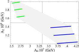
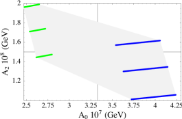
Figure 1: Dependence of $A_{0}$ and $A_{2}$ on $\left\langle\bar{q}q\right\rangle$, $\left\langle GG\right\rangle$, $\Lambda^{(4)}_{\rm QCD}$ and $M$ at $\mu=0.8$ GeV. The gray and black sets of lines correspond to the extreme values of $\Lambda_{\rm QCD}$ and $M$. The length of the lines represents the effect of varying $\left\langle\bar{q}q\right\rangle$, while keeping all other parameters fixed. The vertical spread corresponds to varying $\left\langle\alpha_{s}GG/\pi\right\rangle$, with the central line corresponding to the central value of $\left\langle GG\right\rangle$. The gray area denotes the region spanned by varying all the parameters without correlations in a $\pm$ 30% box around the experimental values of $A_{0}$ and $A_{2}$ given by the cross hairs. The figure shows the HV and NDR results, corresponding to varying $\left\langle\bar{q}q\right\rangle$, $\left\langle GG\right\rangle$, $\Lambda^{(4)}_{\rm QCD}$ and $M$ in the ranges given in eqs. (13)–(14).

Hadronic matrix elements in the $\chi$QM depend on the $\gamma_{5}$-scheme utilized [10]. Their dependence partially cancels that of the short-distance NLO Wilson coefficients. Because this compensation is only numerical, and not analytical, we take it as part of our phenomenological approach. A formal $\gamma_{5}$-scheme matching can only come from a model more complete than the $\chi$QM. Nevertheless, the result, as shown in Fig. 2, is rather convincing.

By taking

$$\Lambda^{(4)}_{\rm QCD}=340\pm 40\ \mbox{MeV}$$

and fitting at the scale $\mu=0.8$ GeV the amplitudes in eqs. (3)–(12) to their experimental values, allowing for a $\pm$ 30% systematic uncertainty, we find (see Fig. 1)

$$M = 195^{+25}_{-15}\;\mbox{MeV}\,,$$

$$\langle\alpha_{s}GG/\pi\rangle = \left(330\pm 5\>\>\mbox{MeV}\right)^{4}\,,$$

$$\langle\bar{q}q\rangle = \left(-235\pm 25\>\>\mbox{MeV}\right)^{3}\;.$$ (13)

in the HV-scheme, and

$$M = 195^{+15}_{-10}\;\mbox{MeV}\,,$$

$$\langle\alpha_{s}GG/\pi\rangle = \left(333^{+7}_{-6}\>\>\mbox{MeV}\right)^{4}\,,$$

$$\langle\bar{q}q\rangle = \left(-245\pm 15\>\>\mbox{MeV}\right)^{3}\;.$$ (14)

in the NDR-scheme.

As shown by the light (NDR) and dark (HV) curves in Fig. 2, the $\gamma_{5}$-scheme dependence is controlled by the value of $M$, the range of which is fixed thereby. The $\gamma_{5}$ scheme dependence of both amplitudes is minimized for $M\simeq 190-200$ MeV. The good $\gamma_{5}$-scheme stability is also enjoyed by $\varepsilon^{\prime}/\varepsilon$ and $\hat{B}_{K}$.

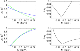
Figure 2: Test of the $\gamma_{5}$-scheme stability of the $A_{0}$ and $A_{2}$ amplitudes as functions of $M$. The light (dark) curves correspond to the NDR (HV) results, while the horizontal lines mark the experimental values. The two figures on the right plot $\Delta A_{I}\equiv 2|(A_{I}^{HV}-A_{I}^{NDR})/(A_{I}^{HV}+A_{I}^{NDR})|$. For the values of $\left\langle\bar{q}q\right\rangle$ and $\left\langle\alpha_{s}GG/\pi\right\rangle$ in eqs. (13)–(14) we find $\gamma_{5}$-scheme independence for $M\simeq 190-200$ MeV.

The fit of the amplitude $A_{0}$ and $A_{2}$ is obtained for values of the quark and gluon condensates which are in agreement with those found in other approaches, i.e. QCD sum rules and lattice, although the relation between the gluon condensate of QCD sum rules and lattice and that of the $\chi$QM is far from obvious. The value of the constituent quark mass $M$ is in good agreement with that found by fitting radiative kaon decays [14].

In Fig. 3 we present the anatomy of the relevant operator contributions to the $CP$ conserving amplitudes. It is worth noticing that, because of the NLO enhancement of the $I=0$ matrix elements (mainly due to the chiral loops), the gluon penguin contribution to $A_{0}$ amounts to about 20% of the amplitude.

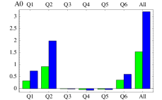
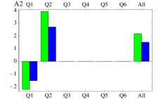
Figure 3: Operator-by-operator contributions to $A_{0}\times 10^{7}$ and $A_{2}\times 10^{8}$ (GeV) in the HV scheme. In (light) dark the (LO) NLO value. Notice the $O(p^{4})$ enhancement of the gluon penguin operator in the $I=0$ amplitude.

Turning now to the $\Delta S=2$ Lagrangian, by using the input values found by fitting the $\Delta I=1/2$ rule we obtain in both $\gamma_{5}$-schemes

$$\hat{B}_{K}=1.1\pm 0.2\,.$$ (15)

The result (15) includes chiral corrections up to $O(p^{4})$ and it agrees with what we found in [10].

Notice that no estimate of $\varepsilon^{\prime}/\varepsilon$ can be considered complete unless it also gives a value for $\hat{B}_{K}$. The case of the $\chi$QM, for instance, is telling insofar as the enhancement of $B_{6}$ is partially compensated for by a large $\hat{B}_{K}$ (and accordingly a smaller $\mathop{\mbox{Im}}\lambda_{t}$).

3.1 The bag parameters $B_{i}$

The bag parameters $B_{i}$, defined as

$$B_{i}\equiv\langle Q_{i}\rangle^{\rm model}/\langle Q_{i}\rangle^{\rm VSA}\,,$$ (16)

have become a standard way of displaying the values of the hadronic matrix elements in order to compare them among various approaches. However they must be used with care because of their dependence on the renormalization scheme and scale, as well as on the choice of the VSA parameters.

	HV	NDR
$B^{(0)}_{1}$	$9.3$	$9.7$
$B^{(0)}_{2}$	$2.8$	$2.9$
$B^{(2)}_{1}=B^{(2)}_{2}$	$0.42$	$0.39$
$B_{3}$	$-2.3$	$-3.0$
$B_{4}$	1.9	1.3
$B_{5}\simeq B_{6}$	$1.8\times\frac{(-240\ {\rm MeV})^{3}}{\left\langle\bar{q}q\right\rangle}$	$1.3\times\frac{(-240\ {\rm MeV})^{3}}{\left\langle\bar{q}q\right\rangle}$
$B_{7}^{(0)}\simeq B_{8}^{(0)}$	$2.6$	$2.4$
$B_{9}^{(0)}$	$3.5$	$3.4$
$B_{10}^{(0)}$	$4.3$	$5.2$
$B_{7}^{(2)}\simeq B_{8}^{(2)}$	$0.89$	$0.84$
$B_{9}^{(2)}=B_{10}^{(2)}$	$0.42$	$0.39$

Table 1: Central values of the $B_{i}$ factors in the HV and NDR renormalization schemes. For $B_{5,6}$ the leading scaling dependence on $\left\langle\bar{q}q\right\rangle$ is explicitly shown for a conventional value of the condensate. All other $B_{i}$ factors are either independent or very weakly dependent on $\left\langle\bar{q}q\right\rangle$. The dependence on $\left\langle\alpha_{s}GG/\pi\right\rangle$ in the ranges of eqs. (13)–(14) remains always below 10%.

They are given in the $\chi$QM in table 1 in the HV and NDR schemes, at $\mu=0.8$ GeV, for the central value of $\Lambda_{\rm QCD}^{(4)}$. The uncertainty in the matrix elements of the penguin operators $Q_{5-8}$ arises from the variation of $\left\langle\bar{q}q\right\rangle$. This affects mostly the $B_{5,6}$ parameters because of the leading linear dependence on $\left\langle\bar{q}q\right\rangle$ of the $Q_{5,6}$ matrix elements in the $\chi$QM, contrasted to the quadratic dependence of the corresponding VSA matrix elements. Accordingly, $B_{5,6}$ scale as $\langle\bar{q}q\rangle^{-1}$, or via PCAC as $m_{q}$, and therefore are sensitive to the value chosen for these parameters. For this reason, we have reported the corresponding values of $B_{5,6}$ when the quark condensate in the VSA is fixed to its PCAC value. It should however be stressed that such a dependence is not physical and is introduced by the arbitrary normalization on the VSA result. The estimate of $\varepsilon^{\prime}$ is therefore almost independent of $m_{q}$, which only enters the NLO corrections and the determination of $\hat{B}_{K}$.

The enhancement of the $Q_{5,6}$ matrix elements with respect to the VSA values—the conventional normalization of the VSA matrix elements corresponds to taking $\left\langle\bar{q}q\right\rangle$$(0.8\ {\rm GeV})\simeq(-220\ {\rm MeV})^{3}$—is mainly due to the NLO chiral loop contributions. Such an enhancement, due to final state interactions, has been found in $1/N_{c}$ analyses beyond LO [15, 16], as well as old and recent dispersive studies [17].

4 Bounds on $\mathop{\mbox{Im}}\lambda_{t}$

The updated measurements for the CKM elements $|V_{ub}/V_{cb}|$ implies a change in the determination of the Wolfenstein parameter $\eta$ that enter in $\mathop{\mbox{Im}}\lambda_{t}$. This is of particular relevance because it affects proportionally the value of $\varepsilon^{\prime}/\varepsilon$.

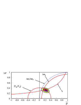
Figure 4: Bounds on the Wolfenstein parameters $\bar{\eta}\equiv(1-\lambda^{2}/2)$ and $\bar{\rho}\equiv(1-\lambda^{2}/2)$ and distribution of $\mathop{\mbox{Im}}\lambda_{t}$ according to Parodi et al. for the input parameters in [22].

The allowed values for $\mathop{\mbox{Im}}\lambda_{t}\simeq\eta|V_{us}||V_{cb}|^{2}$ are found by imposing the experimental constraints for $\varepsilon$, $|V_{ub}/V_{cb}|$, $\Delta m_{d}$ and $\Delta m_{s}$. By using the method of Parodi, Roudeau and Stocchi [18], who have run their program starting from our inputs listed in [22], it is found that

$$\mathop{\mbox{Im}}\lambda_{t}=(1.14\pm 0.11)\times 10^{-4}\,,$$ (17)

where the error is determined by the Gaussian distribution in Fig. 4.

5 Estimating $\varepsilon^{\prime}/\varepsilon$ 

The value of $\varepsilon^{\prime}$ computed by taking all input parameters at their central values is shown in Fig. 5. The figure shows the contribution to $\varepsilon^{\prime}$ of the various operators in two $\gamma_{5}$ renormalization schemes at $\mu=0.8$ GeV and $1.0$ GeV. The advantage of such a histogram is that, contrary to the $B_{i}$, the size of the individual contributions does not depend on some conventional normalization.

As the histogram makes it clear, the gluon-penguin operator $Q_{6}$ dominates and there is very little cancellation with the electroweak penguin operator $Q_{8}$. The dominance of the $I=0$ components in the $\chi$QM originates from the $O(p^{4})$ chiral corrections, the detailed size of which is determined by the fit of the $\Delta I=1/2$ rule. It is a nice feature of the approach that the renormalization scheme stability imposed on the $CP$ conserving amplitudes is numerically preserved in $\varepsilon^{\prime}/\varepsilon$. The comparison of the two figures shows also the remarkable renormalization scale stability of the central value once the perturbative running of the quark masses and the quark condensate is taken into account.

In what follows, the model-dependent parameters $M$, $\left\langle\alpha_{s}GG/\pi\right\rangle$ and $\left\langle\bar{q}q\right\rangle$ are uniformly varied in their given ranges (flat scanning), while the others are sampled according to their normal distributions. Values of $\varepsilon^{\prime}/\varepsilon$ found in the HV and NDR schemes are included with equal weight.

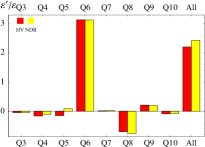
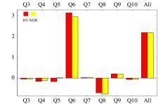
Figure 5: Contribution to $\varepsilon^{\prime}/\varepsilon$  (in units of $10^{-3}$) of each penguin operator in the HV and NDR $\gamma_{5}$-schemes. The figure on the left (right) corresponds to $\mu=0.8$ ($1.0$) GeV.

For a given set, a distribution is obtained by collecting the values of $\varepsilon^{\prime}/\varepsilon$ in bins of a given range. This is shown in Fig. 6 for a particular choice of bins. Because the skewness of the distribution is less than one, the mean and the standard deviation are a good estimate of the central value and the dispersion of values around it.

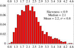
Figure 6: Distribution of values of $\varepsilon^{\prime}/\varepsilon$ (in units of $10^{-3}$). Normalized bins are plotted against the values of $\varepsilon^{\prime}/\varepsilon$ of each bin.

This statistical analysis yields

$$\varepsilon^{\prime}/\varepsilon=(2.2\pm 0.8)\times 10^{-3}\,.$$ (18)

A more conservative estimate of the uncertainties is obtained via the flat scanning of the input parameters, which gives

$$0.9\times 10^{-3}<\mathop{\mbox{Re}}\>\varepsilon^{\prime}/\varepsilon<4.8\times 10^{-3}\,.$$ (19)

In both estimates a theoretical systematic error of $\pm 30\%$ is included in the fit of the $CP$ conserving amplitudes $A_{0}$ and $A_{2}$.

The stability of the numerical outcomes is only marginally affected by shifts in the value of $\Omega_{\eta+\eta^{\prime}}$. Any effective variation of $\Omega_{\eta+\eta^{\prime}}$ is anti-correlated to the value of $\left\langle\alpha_{s}GG/\pi\right\rangle$ obtained in the fit of $A_{2}$. We have verified that this affects the calculation of $\hat{B}_{K}$ and the consequent determination of $\mathop{\mbox{Im}}\lambda_{t}$ in such a way to compensate numerically in $\varepsilon^{\prime}/\varepsilon$ the change of $\Omega_{\eta+\eta^{\prime}}$. Waiting for a confident assessment of the NLO isospin violating effects in the $K\to\pi\pi$ amplitudes, we have used for $\Omega_{\eta+\eta^{\prime}}$ the ‘LO’ value $0.25\pm 0.10$.

The weak dependence on some poorly-known parameters is a welcome outcome of the correlation among hadronic matrix elements enforced in our semi-phenomenological approach by the fit of the $\Delta I=1/2$ rule.

While the $\chi QM$ approach to the hadronic matrix elements relevant in the computation of $\varepsilon^{\prime}/\varepsilon$ has many advantages over other techniques and has proved its value in the prediction of what has been then found in the experiments, it has a severe short-coming insofar as the matching scale has to be kept low, around 1 GeV and therefore the Wilson coefficients have to be run down at scales that are at the limit of the applicability of the renormalization-group equations. Moreover, the matching itself suffers of ambiguities that have not be completely solved. For these reasons we have insisted all along that the approach is semi-phenomenological and that the above shortcomings are to be absorbed in the values of the input parameters on which the fit to the $CP$ conserving amplitudes is based. Because of its simplicity, the $\chi$QM is clearly not the final word and it can now been abandoned—as a ladder used to climb a wall after we are on the other side—as we work for better estimates, in particular, those from the lattice simulations.

6 Other estimates

Figure 7 summarizes the present status of theory versus experiment. In addition to the current $\chi$QM calculation (and an independent estimate similarly based on the $\chi$QM), there are eight estimates of $\varepsilon^{\prime}/\varepsilon$ published in the last year. Trieste’s, München’s and Roma’s ranges are updates of their respective older estimates, while the others are altogether new.

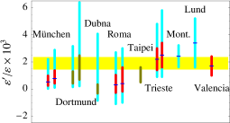
Figure 7: Theory vs. experiment in the year 2000. The gray band is the average experimental result. See [19], [20], [15], [13], [21], [24], [25], [23] for details on the various estimates.

The estimates reported are discussed in [22]. The effects first pointed out by the $\chi$QM have been taken up and refined by some of the other approaches, in particular: non-factorizable corrections [15, 13, 21, 25] and FSI [15, 13, 23]. Figure 7 makes clear that, except for estimates heavily based on VSA for the crucial operator $Q_{6}$, all other estimates are in agreement with the experiments.

References

- [1] B. Winstein and L. Wolfenstein, Rev. Mod. Phys. 65 (1993) 1113.
- [2] G. Buchalla and A. J. Buras and M. E. Lautenbacher Rev. Mod. Phys. 68 (1996) 1125.
- [3] S. Bertolini, J. Eeg and M. Fabbrichesi Rev. Mod. Phys. 72 (2000) 65.
- [4] A. J. Buras et al, Nucl. Phys. B370 (1992) 69 and Nucl. Phys. B400 (1993) 37; A. J. Buras, M. Jamin and M.E. Lautenbacher Nucl. Phys. B400 (1993) 75 and Nucl. Phys. B408 (1993) 209; M. Ciuchini et al. Nucl. Phys. B415 (1994) 403.
- [5] KTeV Collaboration (A. Alavi-Harati et al.) Phys. Rev. Lett. 83 (1999) 22.
- [6] NA48 Collaboration (V. Fanti et al.) Phys. Lett. B465 (1999) 335; (A. Ceccucci) http://www.cern.ch/NA48/Welcome.html.
- [7] NA31 Collaboration (G. D. Barr et al.) Phys. Lett. B317 (1993) 233.
- [8] E731 Collaboration (L. K. Gibbons et al.) Phys. Rev. D55 (1997) 6625.
- [9] M. Fabbrichesi, hep-ph/9909224, published in Nucl. Phys. Proc. Suppl. 86 (200) 322.
- [10] S. Bertolini et al. Nucl. Phys. B514 (1998) 63 and 93.
- [11] K. Nishijima N. Cim. 11 (1959) 698; F. Gursey N. Cim. 16 (1960) 23 and Ann. Phys. 12 (1961) 91; J. A. Cronin Phys. Rev. 161 (1967 1483; S. Weinberg Physica 96A (1979) 327; A. Manohar and H. Georgi Nucl. Phys B234 (1984) 189; A. Manohar and G. Moore Nucl. Phys B243 (1984) 55; D. Espriu et al. Nucl. Phys B345 (1990) 22.
- [12] Y. Nambu and G. Jona-Lasinio Phys. Rev. 122 (1961) 345; J. Bijnens Phys. Rept. 265 (1996) 369.
- [13] A. A. Bel’kov et al. hep-ph/9907335.
- [14] J. Bijnens Int. J. Mod. Phys. A8 (1993) 3045.
- [15] T. Hambye et al. Nucl. Phys. B564 (2000) 391; hep-ph/0001088.
- [16] J. Bijnens and J. Prades JHEP 9901 (1999) 023.
- [17] T. N. Troung Phys. Lett B207 (1988) 495; E. Pallante and A. Pich Phys. Rev. Lett. 84 (2000) 2568 and hep-ph/0007208; J. F. Donoghue and E. Golowich Phys. Lett. B 478 (2000) 172; E. A. Paschos hep-ph/9912230.
- [18] P. Paganini et al. Phys. Scripta 58 (1998) 556; F. Parodi, P. Roudeau and A. Stocchi N. Cim. A112 (1999) 833.
- [19] S. Bosch et al. Nucl. Phys. B565 (2000) 3.
- [20] M. Ciuchini et al. Nucl. Phys. B573 (2000) 201.
- [21] H.-Y. Cheng Mod. Phys. Lett. A14 (1999) 2453.
- [22] S. Bertolini et al.hep-ph/0002234; M. Fabbrichesi hep-ph/0002235.
- [23] E. Pallante and A. Pich, hep-ph/0007208.
- [24] S. Narison, hep-ph/0004247.
- [25] J. Bijnens and J. Prades hep-ph/0005189.