LYCEN 2000-93

September 2000

Damping of the HERA effect in DIS ?

P. Desgrolard ^a,, A. Lengyel ^b,, E. Martynov ^c,

^a Institut de Physique Nucléaire de Lyon, IN2P3-CNRS et Université Claude Bernard, 43 boulevard du 11 novembre 1918, F-69622 Villeurbanne Cedex, France

^b Institute of Electron Physics, National Academy of Sciences of Ukraine, 08015 Uzhgorod-015, Universitetska 21, Ukraine

^c Bogoliubov Institute for Theoretical Physics, National Academy of Sciences of Ukraine, 03143 Kiev-143, Metrologicheskaja 14b, Ukraine

Abstract The drastic rise of the proton structure function $F_{2}(x,Q^{2})$ when the Björken variable $x$ decreases, seen at HERA for a large span of $Q^{2}$, negative values for the 4-momentum transfer, may be damped when $Q^{2}$ increases beyond $\sim$ several hundreds GeV². A new data analysis and a comparison with recent models for the proton structure function is proposed to discuss this phenomenon in terms of the derivative $\partial{\ell nF_{2}(x,Q^{2})}/\partial{\ell n(1/x)}$.

1 Introduction

The so-called ”HERA effect” discovered some years ago by the experimentalists in deep inelastic scattering (DIS) and anticipated by a number of theoreticians has arisen a great interest in the community (see e.g.[1] and references therein). It concerns the strong rise of the proton structure functions (SF) $F_{2}(x,Q^{2})$ when the Björken variable $x$ decreases, for the experimentally investigated $Q^{2}$, negative values for the 4-momentum transfer.

A slow-down of a further rise is inevitable, as a consequence of unitarity, if however the Froissart-Martin [2] bound is valid for $\gamma^{*}p$ interaction at least at $x\to 0$. In this case a power-like behavior of SF at small-$x$ must be transformed into a logarithmic-like one (like in hadron amplitudes, when a procedure of unitarization or eikonalization is applied). Evidently, such an evolution leads to a damping of the fast growth of SF at $x\to 0$.

A natural question arises : will this HERA effect still subsist in any $x-Q^{2}$ region to be investigated, or more pragmatically in which kinematical region a damping is to be expected ?

It is not easy to exhibit this interesting tendency in the behavior of $F_{2}(x,Q^{2})$ at small $x$ and rising $Q^{2}$. This effect is very weak because a sufficient amount of data at high $Q^{2}$ is still lacking. Furthermore, it may stand near the kinematical limit at the available energies (it is the case at HERA ), thus preventing a clear evidence on the basis of existing data. Nevertheless, one can guess it by simply inspecting by eye the evolution of the icons showing the experimental SF versus $x$ at given $Q^{2}$ increasing up to the highest values (see in Fig.1 such a representation using a double logarithmic scale); if this inspection seems inconclusive, one can at least insure that no contradiction appears.

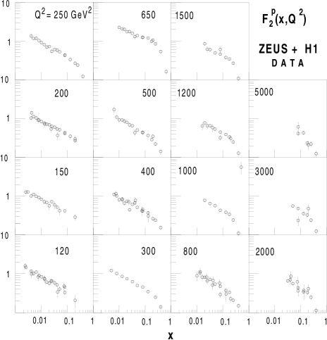
Figure 1: Experimental data of ZEUS and H1 collaborations at high $Q^{2}$

Aside from this empirical mean, a way to quantify the preceding effect is to consider the derivative of the logarithm of the proton SF with respect to $\ell n(1/x)$ ($x-$slope for brevity) defined as

$$B_{x}(x,Q^{2})={\partial\ell nF_{2}(x,Q^{2})\over\partial{\ell n(1/x)}}\ ;$$ (1)

the damping of the HERA effect would correspond to the presence of a maximum when plotting $B_{x}$ versus $Q^{2}$ for a given low $x$.

It is worth noting that this derivative is related to an ”effective power” (exponent of $1/x$) $\Delta$, sometimes labelled $\lambda$, introduced when redefining the proton SF as

$$F_{2}(x,Q^{2})=G(Q^{2})\ \left({1\over x}\right)^{\Delta(x,Q^{2})}\ ,$$ (2)

or in other terms to a Pomeron ”effective intercept” $\alpha_{\cal P}^{eff}$ (depending on $x$ and $Q^{2}$)

$$\alpha_{\cal P}^{eff}(x,Q^{2})=1+\Delta(x,Q^{2})\ .$$ (3)

We emphasize that we can identify $B_{x}=\Delta$, only in the case of a model where $\Delta$ is $x$-independent; in general $B_{x}$ and $\Delta$ do not coincide. A careful analysis of experimental data, based on a comparison of various parametrizations of the SF, has suggested [3] a possible slowing down of the SF rise revealed as a growth of $F_{2}$ with decreasing $x$ becoming steeper and steeper (when $Q^{2}$ rises) which is changed at $Q^{2}\sim 200-500$ GeV² into a growth saturating and even becoming less and less steep at further increasing $Q^{2}$.

From a phenomenological point of view, many parametrizations of the proton structure functions successfully accommodated for the whole - or a part of - available data set and in particular for the steep rise of the SF when $x$ decreases for a large span of $Q^{2}$ values (see e.g.  [4-17]). Several of them have given explicitly some hints (see e.g.  [10, 16, 17]) on the existence of a slowing down of the HERA effect.

We believe that the region of the contour $x-Q^{2}$ plane with $x\mathrel{\hbox to0.0pt{\lower 4.0pt\hbox{\hskip 1.0pt$\sim$}\hss}\raise 1.0pt\hbox{$<$}}10^{-1}$ and $Q^{2}\mathrel{\hbox to0.0pt{\lower 4.0pt\hbox{\hskip 1.0pt$\sim$}\hss}\raise 1.0pt\hbox{$>$}}100$ GeV² is of particular interest for the above question. Happily, recent measurements of SF have become available, from H1 and ZEUS collaborations which fulfil partly this kinematical criterion. They complete or correct the previous data near the HERA collider [18, 19, 20, 21] and [22, 23, 24, 25] and from fixed target experiments [26, 27, 28, 29, 30].

Here, we actualize the conclusions of previous paths driving towards the existence of a damping effect. We perform with new data a relevant analysis similar to [3], where, however, only the averaged slopes $B_{x}(x,Q^{2})$ were determined in almost the whole available interval of $x$ at given fixed $Q^{2}$.

It is necessary to remark here that the data on $\lambda_{eff}$ [24] cannot be interpreted as showing a dependence of the effective intercept ($\Delta_{eff}(Q^{2})$) on $Q^{2}$. Each point $B_{x}$ has not been extracted at the same $<x>$, There is an evident correlation between the values of $Q^{2}$ and of the corresponding $<x>$, namely a larger $<x>$ corresponds to a larger $Q^{2}$ for almost all points . To exhibit a true dependence of the effective intercept on $Q^{2}$, one need to have the local $B_{x}$ extracted at the same $<x>$ but for different $Q^{2}$. It is one of the reasons motivating the present work. We attempt a new, more detailed, systematic (on all available data) and model independent analysis of the local slope $B_{x}(x,Q^{2})$ having in mind its possible variation with $x$. It allows not only to extract the averaged slopes at fixed $Q^{2}$ but also to determine the dependence of $B_{x}(x,Q^{2})$ on $Q^{2}$ at fixed $x$.

We also turn towards three basically different phenomenological models for the proton SF, namely: the ”ALLM” model [5], the ”interpolating Lyon-Kiev-Padova” (LKP) model [16], the ”soft dipole Pomeron” (DP) model [17], and have been refitted (or eventually improved as concerns LKP) with a common set of data including the most recent ones, their predictions concerning the $x-$slope are compared to the results of the present analysis.

2 Models for the proton structure functions

2.1 Common set of data included in the fitting procedure

The choice of the data set used in the fits may have crucial consequences when calculating the derivatives of the SF, especially when this quantity is to be discussed near the experimental kinematical limit or/and near the theoretical validity limit. For these reasons, a unique set including the most recent data has been used in new fits of three models of the proton SF we choose to discuss.

These updated data are listed and referenced in Table 1. The complete available experimental kinematical range is taken into account for $Q^{2}$ (i.e. $0.\leq Q^{2}$ $\leq 30000$ GeV²) and $x$ (i.e. $6.\ 10^{-7}\leq x\leq 0.75$), with the lower limit of the center of mass energy for ${\gamma^{*}p}$ scattering $W\geq 3$ GeV.

$$\begin{array}[]{|cc|c|c|c|}\hline\cr{\rm Observable}&&&\chi^{2}&\chi^{2}\\ {\rm Exp.-year\ of\ pub.,}&{\rm\ Ref}&{\rm Nb\,points}&{\rm model~{}\cite[cite]{[\@@bibref{}{djp}{}{}]}}&{\rm model~{}\cite[cite]{[\@@bibref{}{dlm}{}{}]}}\\ \hline\cr\hline\cr F_{2}^{p}&&&&\\ {\rm H1-1995}&\cite[cite]{[\@@bibref{}{ah95}{}{}]}&93&76.1&70.7\\ {\rm H1-1996}&\cite[cite]{[\@@bibref{}{ai96}{}{}]}&129&90.9&68.9\\ {\rm H1-1997}&\cite[cite]{[\@@bibref{}{ad97}{}{}]}&44&53.0&53.5\\ {\rm H1-1999}&\cite[cite]{[\@@bibref{}{ad99}{}{}]}&130&237.9&111.0\\ {\rm ZEUS-1996}&\cite[cite]{[\@@bibref{}{de96}{}{}]}&188&259.9&261.5\\ {\rm ZEUS-1997}&\cite[cite]{[\@@bibref{}{br97}{}{}]}&34&12.2&17.3\\ {\rm ZEUS-1999}&\cite[cite]{[\@@bibref{}{br99}{}{}]}&44&26.7&38.5\\ {\rm ZEUS-2000}&\cite[cite]{[\@@bibref{}{br00}{}{}]}&70&139.6&79.3\\ {\rm NMC-1997}&\cite[cite]{[\@@bibref{}{ar97}{}{}]}&156&285.5&161.1\\ {\rm E665-1996}&\cite[cite]{[\@@bibref{}{ad96}{}{}]}&91&109.7&99.5\\ {\rm SLAC-1990/92}&\cite[cite]{[\@@bibref{}{slac}{}{}]}&136&193.6&107.3\\ {\rm BCDMS-1989}&\cite[cite]{[\@@bibref{}{be89}{}{}]}&175&274.8&269.9\\ \hline\cr\sigma_{tot}^{\gamma,p}&&&&\\ {\rm 1975/78;ZEUS-1994;H1-1995}&\cite[cite]{[\@@bibref{}{ca75}{}{}]}&99&148.6&122.7\\ \hline\cr{\rm Total}&&1389&1907.6&1461.2\\ \hline\cr\hline\cr\chi^{2}\ /\ d.o.f.&&&1.38&1.07\\ \hline\cr\end{array}$$

Table 1. Observables sets used in the fitting procedure. Also shown are the distributions of the partial $\chi^{2}$ for each subset of data used in our new fits with the parameters listed below in Tables 2-3, for the two updated models [16, 17].

Generally speaking, we must note a good agreement between both HERA experiments, H1 and ZEUS, and the fixed target ones. Following the suggestion from [21], some data from  [19] are considered as obsolete and superseded. These correspond to ($Q^{2}\geq 250$ GeV² , for all $x$), ($Q^{2}=200$ GeV² , for $x<0.1$) and ($Q^{2}=150$ GeV² , for $x<0.01$).

2.2 Parametrizations of the structure function

2.2.1 The ALLM model

The so-called ALLM parametrization [5] for describing the total $\gamma^{*}p$ cross section, connected to the proton SF, has been updated in 1997 to account for the set of available data in the whole range studied so far: $0<Q^{2}<$ 5000 GeV², and $3.10^{-6}<x<0.85$. Here, to make the comparison with the other results more meaningful, we extend the $x,Q^{2}$ ranges over all the data of Table 1 and perform a new fit of the 23 parameters of this model. We find again quite a good agreement which can be characterized by $\chi^{2}_{d.o.f}$=1.06

2.2.2 The Lyon-Kiev-Padova model revisited

We emphasize that this LKP model was created for interpolating between soft and hard dynamics, combining Regge behavior and the high $Q^{2}$ asymptotics of the DGLAP evolution equation, for the low$-x$ range, with a small number of free parameters (8, in [16]).

To improve the quality of the fit on all data, we accept to lose the simplicity of the original model by modifying here the ”large” $x$ extension which is no more borrowed from the relatively simple and rather efficient model [8] but, instead, we follow the more sophisticated approach from [17]. Explicitly, the SF has been rewritten

$$F_{2}(x,Q^{2})=\ F_{2}^{(S,0)}(x,Q^{2})\cdot(1-x)^{P(Q^{2})}+\ F_{2}^{(NS,0)}(x,Q^{2})\cdot(1-x)^{R(Q^{2})}\ ,$$ (4)

where the Pomeron contribution (singlet $F_{2}^{(S,0)}$) and the effective secondary Reggeon component (non-singlet $F_{2}^{(NS,0)}$) have here the same expressions as in [16] at low$-x$, and with the following $Q^{2}$-dependent exponents of the large$-x$ factors

$$P(Q^{2})=\ p_{\infty}+{p_{0}-p_{\infty}\over 1+Q^{2}/Q^{2}_{p}}\ ,\quad R(Q^{2})=\ r_{\infty}+{r_{0}-r_{\infty}\over 1+Q^{2}/Q^{2}_{r}}\ ,$$ (5)

where $p_{\infty},p_{0},r_{\infty},r_{0},Q_{p},Q_{r}$ are thus additional parameters in the present version of the LKP model . In definitive, taking into account the large $x$ in practice doubles the parameters number, but it is the price of such an extension. The details on the performances of this extended model are given in Table 1 in terms of the $\chi^{2}$ for each subset of data, yielding $\chi^{2}_{d.o.f}$=1.38. The parameters we find are listed in the Table 2, with their meaning explained in [16] and above.

Parameters	previous work [16]	present work
low $x-$terms
$A$	$0.1470$	0.1190
$a$ (GeV2)	$0.2607$	0.2300
$\epsilon$	0.08 (fixed)	0.0895
$\gamma_{2}$	$0.0200$	0.0221
$Q_{0}^{2}$ (GeV2)	$0.1675$	0.1946
$Q_{1}^{2}$ (GeV2)	$1174.$	7800.
$B$	$0.7575$	1.6409
$b$ (GeV2)	$0.4278$	1.46
$\alpha_{r}$	$0.5241$	0.48 (fixed)
large $x-$terms	(fixed)
$Q^{2}_{p}$ (GeV2)	$-$	1.1180
$p_{0}$	$-$	$\approx 0.$
$p_{\infty}$	$-$	15.093
$Q^{2}_{r}$ (GeV2)	$-$	12.563
$r_{0}$	$-$	2.394
$r_{\infty}$	$-$	3.728

Table 2. Parameters used in the previous and present versions of the LKP model. The non-fitted values are: $\gamma_{1}=2.4$ (suggested by QCD) for both versions, $\epsilon=0.08$ (from [33]) and the large $x$ exponents (from [8]) for the previous work only.

When the intercept $\alpha_{r}$ of the $f$-Reggeon is allowed to be free we obtained a better $\chi^{2}(\approx 1.22)$. However the resulting value of $\alpha_{r}\approx 0.24$ is totally unacceptable from a physical point of view. For that reason, we fixed it, choosing $\alpha_{r}=0.48$, a ”mean” value used in the models with a supercritical Pomeron.

2.2.3 Soft dipole Pomeron model

The refitted parameters of this model are given in Table 3 together with the old ones published in [17] (the same notations are used). The most interesting property of this model developed in [17] is the intercept of Pomeron. It does not depend on $Q^{2}$ and moreover it is equal to one. Nevertheless due to an interference of two Pomeron components, the model describes well all observed properties of the proton structure function, including a growth with $Q^{2}$ of the effective Pomeron intercept (see for details [17] and [31]). The first Pomeron component, dominating at small $x$, leads to $F_{2}(x,Q^{2})\propto\ell n(1/x)$ at $x\to 0$ while the second one gives asymptotically a constant and negative contribution to $F_{2}$ playing an important role in the whole kinematic region where the data on the proton SF data are available.

Parameters	previous work [17]	present refit
$P_{1}$-term
$\mu$	.10000E+01 (fixed)	.10000E+01 (fixed)
$\alpha_{\cal P}(0)$	.10000E+01 (fixed)	.10000E+01 (fixed)
$g_{1}$ (mb$)$	.21898E-01	.22198E-01
$Q_{1}^{2}$ (GeV${}^{2})$	.15400E+02	.70711E+01
$Q_{1d}^{2}$ (GeV${}^{2})$	.17852E+01	.14774E+01
$Q_{1b}^{2}$ (GeV${}^{2})$	.33435E+01	.67975E+01
$d_{1\infty}$	.13301E+01	.12601E+01
$d_{10}$	.14370E+02	.66975E+01
$b_{1\infty}$	.21804E+01	.28712E+01
$b_{10}$	.42596E+01	-.20279E+01 (fixed)
$P_{2}$-term
$g_{2}$ (mb)	-.99050E-01	-.10176E+00
$Q_{2}^{2}$ (GeV${}^{2})$	.34002E+02	.13748E+02
$Q_{2d}^{2}$ (GeV${}^{2})$	.12327E+01	.15954E+01
$Q_{2b}^{2}$ (GeV${}^{2})$	.20702E-01	.80605E+01
$d_{2\infty}-d_{1\infty}$	.00000E+00 (fixed)	.00000E+00 (fixed)
$d_{20}$	.22607E+02	.64794E+01
$b_{2\infty}$	.24686E+01	.34510E+01
$b_{20}$	.17023E+03	.12922E+01
$F$-term
$\alpha_{f}(0)$	.80400E+00 (fixed)	.80400E+00 (fixed)
$g_{f}$ (mb)	.29065E+00	.29405E+00
$Q_{f}^{2}$ (GeV${}^{2})$	.29044E+02	.10182E+02
$Q_{fd}^{2}$ (GeV${}^{2})$	.54462E+00	.70413E+00
$Q_{fb}^{2}$ (GeV${}^{2})$	.20656E+01	.84803E+00
$d_{f\infty}$	.13554E+01	.13149E+01
$d_{f0}$	.75127E+02	.19746E+02
$b_{f\infty}$	.27239E+01	.33642E+01
$b_{f0}$	.64713E+00	-.27968E+01 (fixed)

Table 3. Parameters refitted in the soft Dipole Pomeron model of [17], the original values are also quoted.

Analyzing the properties of the model we found that it is not necessary to restrict the parameters $b_{10},b_{20}$ and $b_{f}$ (which influence the behaviour of $F_{2}$ at $x\to 1$) to positive values. Indeed, there are two domains when $x\approx 1$. In the first one, $Q^{2}$ is large, $Q^{2}\gg W^{2}-m^{2}$, the $x$-behaviour of $F_{2}$ is controlled by $b_{i\infty}$ rather than by $b_{i0}$. In the second domain $W^{2}$ is small, $W^{2}-m^{2}\approx 0$, it is a region where the Regge approach cannot be applied.

Thus, we allowed the negative values for $b_{10},b_{20}$ and $b_{f0}$ and found out a new set of parameters which, though noticeably different from the old one, leads to a very good $\chi^{2}\approx 1.07$.

3 Extracting the local slopes $B_{x}(x,Q^{2})$ from the SF data.

As noted in the introduction, the $x-$slope is a precious tool to settle if, either yes or no, a damping of the HERA effect does exist. Actually, we need a set of experimental data on $B_{x}(x,Q^{2})$, at fixed and not too high $x$ versus sufficiently high $Q^{2}$. Unfortunately, because the $x-$slope is not a measurable observable it should be extracted, when possible, from the available data on the SF.

For each given $Q^{2}$, we have an insufficient number of $x$ values for which SF data are available, to perform an analysis based on independent $x-$ bins and to extract $x$-slopes with a good accuracy. We adapt the so-called method of ”overlapping bins” [32], previously intended for analyzing the local nuclear slope of the first diffraction cone in $pp$ and $\bar{p}p$ elastic scattering.

Provided that the SF has been measured for a given $Q^{2}$ at $N$ $x$-points lying in some interval $[x_{min},x_{max}]$, we adopt the following procedure. First, we divide this interval into subintervals or elementary ”bins” (with $n_{b}$ measurements in each of them, assumed for simplicity to be the same for all bins). When the first bin is chosen, the second bin is obtained from the first by shifting only one point of measurement (of course one could shift bins by any number of points less or equal $n_{b}$, the shift of one point is the minimal one giving rise to the maximal number of overlapping bins). The third bin is obtained from the second one by the shift of one point etc… Thus, we define $N-n_{b}+1$ overlapping bins for a given $Q^{2}$. For each ($k$-th) bin, $n_{b}$ must be large enough and its width (in $x$) small enough to allow fitting the SF with the simplest form directly involving the $x-$slope

$$F_{2}(x)=A\left({1\over x}\right)^{B}\ ,\quad({\rm for\ a\ given}\ Q^{2})\ .$$ (6)

The parameter $B$ represents the value of the $x-$slope $B\left(<x>_{k},Q^{2}\right)$, ”measured”, at $Q^{2}$ and at the ”weighted average” $<x>_{k}$ defined in the $k$-th bin as (see [24])

$$<x>_{k}=exp\bigg{(}-{\sum{\ln x_{i}\over\Delta y_{i}}\over\sum{1\over\Delta y_{i}}}\bigg{)}\ ,\quad k\in{[1,N-n_{b}+1]}\ ,$$ (7)

where $x_{i}$ is the value of $x$ at which the structure function $y_{i}$ is measured with the uncertainty $\Delta y_{i}$; the summations run over all data points, $i=1,2,...,n_{b}$ of the bin. This yield the ”experimental” values of $B_{x}(x,Q^{2})$ with the corresponding standard errors determined in the fit of (6) to the data. Then the procedure is to be repeated for all bins and ultimately for the other $Q^{2}$’s at which the SF have been measured.

The next step in extracting and analyzing $B_{x}(x,Q^{2})$ is the determination of the slopes at fixed $x$ as function of $Q^{2}$, making use of results of the first step. As a rule, the sets of $<x>_{k}$, at different $Q^{2}$, do not coincide. So in order to get the $x-$slope at fixed $x$ and at different $Q^{2}$ we interpolate (or extrapolate but not far from the $x$-interval under consideration) already extracted $B_{x}$ at the given $Q^{2}$ to the chosen $x$. It can be made assuming a linear $x-$dependence of $B_{x}$.

The above mentioned method of overlapping bins is applied to the whole available data set. The HERA data (of ZEUS and H1) are analyzed all together [18-25] but independently (separately) from older data of the other experimental Collaborations [26-30] because there are large gaps between the $x$-values for these two groups of data (remind that our aim is to extract the local $B_{x}$ rather than averaged ones).

The resulting values of $B_{x}(x,Q^{2})$ are shown in the Figs .2 (a-e), where they are compared to the predictions of theoretical models. The results of the interpolation for $x=0.005,0.01,0.05$ and 0.08 are presented in the Fig. 3.

We would like to comment some ”technical” points in our analysis and results.

• In order to keep its local character to the $x$-slope and to obtain a maximal possible number of ”measurements”, we have considered only the cases with four and five points in each elementary bin. One can see from the presented figures a quite weak dependence of the results on a change in the width of elementary bin.

• In spite of a high accuracy of the recent data from HERA, the dispersion of the SF-values strongly influences the resulting values of $B_{x}$ and of its errors. For some bins, for example, we were unable to fit (6) to the data with $\chi^{2}\leq 1$, so we could not obtain in all cases reasonable errors. Nevertheless we show these extracted values (only with $\chi^{2}\leq 3$)in the figures and use them for interpolation to the $x$ under interest because even with these points the extracted set of data for $B_{x}(x,Q^{2})$ at fixed $x$ is quite poor. Of course, this reduces the reliability of our results, but only slightly because the number of ”bad” bins remains small.

• ”Experimental” values of $B_{x}$ at fixed $x$ shown in Fig. 3 are obtained by a linear interpolation within the two subsets of local $x$-slopes, extracted from the HERA and from the fixed target measurements of SF.

• One can see in Fig. 3 that several points deviate strongly from the groups constituted by the other points. This is due to the strong influence of the points (of $F_{2}$ as well as of $B_{x}$) which are at the ends of the $x$-bins and which also ”fall out of a common line” (see also item ii) above). To solve this problem, a possible way would be to exclude some of them from the analysis; another way would be to enlarge the number of points in an elementary bin losing, however, the local character of the extracted $x-$slope. A more detailed analysis of the available data related to more numerous measurements of the primary observable, $F_{2}(x,Q^{2})$ would be necessary to obtain a better set of data for $B_{x}(x,Q^{2})$.

(a)

Fig. 2 (a-e). The $x-$slopes $B_{x}(x,Q^{2})$ at fixed $Q^{2}$ and versus $x$, extracted from the experimental data on the structure function by the method of overlapping bins. Triangles ($n_{b}=5$) and circles ($n_{b}=4$) correspond to the slopes extracted from the HERA data. Stars ($n_{b}=5$) and diamonds ($n_{b}=4$) are the slopes extracted from fixed target data. Curves are predictions in the DP (solid line), ALLM (dashed line) and LKP (dashed-dotted line) models.

(b)

(d)

(c)

(e)

Fig. 3. The slopes $B_{x}$ interpolated to some $x$-s as function of $Q^{2}$. The vertical dotted lines show the HERA kinematical limits for given $x$. See Fig. 2.

4 Results and discussion

The calculated $x-$slopes within the three models are in good agreement with the values extracted from the experimental SF via the present analysis (in the data bars, see Figs .2), except at largest $x$ where the predictions are slightly higher than experimental points.

Except for the highest $Q^{2}$, in Fig. 2(e), and for the lowest $x$ in all figures, the theoretical curves almost coincide. To that respect, the slope does not appear as a good criterion for discriminating among the various models. However, we found that the three models predict noticeably different $x-$slopes when $x$ is very small, outside reported experimental range (the difference growing when $x$ decreases) . For example, we find $B_{x}(x=10^{-4},Q^{2}=100\mbox{GeV}^{2})\approx 0.2$ for DP, $\approx 0.4$ for LKP, and $\approx 0.3$ for ALLM.

Thus, an extension of the $x,Q^{2}$ range for $B_{x}$ towards small $x$, requiring much effort in measuring and analyzing the FS, would be very interesting to seek the experimental evidence of the validity (or non validity) of the Froissart-Martin bound in deep inelastic scattering by ensuring whether (or not) $B_{x}(x\to 0,Q^{2})\to 0$. Furthermore, exploration of this kinematical region allows to select a model upon experimental grounds.

The damping effect is characterized by a slowing down of the $x-$slope growth, when $Q^{2}$ increases for any $x$, resulting in a turn-over in the behavior of th $x-$slope.

From the theoretical point of view, we recall that we tested only three models [5, 16, 17], which assume quite different asymptotic behaviors of the SF and consequently of $B_{x}(x\ll 1,Q^{2}\to\infty)$ (for more details see [17]). The Fig. 3 shows the $x-$slope calculated in these models and plotted versus $Q^{2}$, for some $x-$ values. Only LKP and DP models do predict  a bump in the curve for $Q^{2}$ above 100 GeV², ALLM does not : consequently, we cannot rely on theoretical predictions alone due to that model dependence.

From the experimental point of view, the figure shows data points resulting from our analysis, seeming to correspond to a maximum. However, the most interesting part of the $Q^{2}$ range to explore in the future (because situated in the downhill of the predicted $x-$slope and allowing to conclude unambiguously) lies above the actual measurements and not too far from the actual kinematical limit (at least for HERA facilities).

We conclude that a deeper theoretical knowledge of the high energy positron-proton interaction or/and more precise measurements and analysis, opened in higher $Q^{2}$ range, are needed to confirm or to disprove without ambiguity a bump structure in the behavior of $B_{x}(x,Q^{2})$ at small fixed $x$.

Acknowledgements We have the pleasure to thank L. Jenkovszky for interesting discussions and M. Giffon for a critical reading of the manuscript. E.M. is grateful to Univercité Claude Bernard and IPNL for the kind hospitality and financial support extended to him during this work.

References

- [1] A. Levy, DESY 97-013 (1997).
- [2] M. Froissart, Phys. Rev. 123, 1053 (1961); A. Martin, Nuovo Cim. 42, 930 (1966)
- [3] P.Desgrolard, L. Jenkowzsky, A. Lengyel, F. Paccanoni, Phys. Lett. B 459, 265 (1999)
- [4] L.V. Gribov, E.M. Levin, M.G. Ryskin, Phys. Rep. 100, 1 (1983)
- [5] H. Abramovicz, E.Levin, A. Levy, U. Maor, Phys. Lett. B 269, 465 (1991); H. Abramovicz, A. Levy, DESY 97-251, hep-ph/9712415 (1997)
- [6] B. Badelek, J. Kwiecinski, Phys. Lett. B 295, 263 (1992)
- [7] A. Donnachie, P.V. Landshoff, Zeit. Phys. C 61, 139 (1994)
-
[8]
A. Capella, A. Kaidalov, C. Merino, J. Tran Thanh Van, Phys. Lett. B 337, 358 (1994),
A. Kaidalov, C. Merino, D. Pertermann, On the behavior of and its logarithmic slopes, hep-ph/0004237 - [9] M. Glük, E. Reya, A. Vogt, Zeit. Phys. C 67, 433 (1995)
- [10] M. Bertini et al. , in ”Strong interactions at long distances”, edited by L. Jenkovszky, Hadronic Press, Palm Harbor, FL U.S.A, 1995), p.181
- [11] A. De Roeck, E.A. De Wolf, Phys. Lett. B 388, 863 (1996)
- [12] V. Barone, M. Genovese, N.N. Nikolaev, E. Predazzi, B.G. Zakharov, Zeit. Phys. C 70, 83 (1996)
- [13] S. Aid et al. H1 collaboration, Nucl. Phys. B 470, 3 (1996)
- [14] K. Adel, F. Barreiro, F.J. Yndurain, Nucl. Phys. B 495, 221 (1997)
- [15] D. Schildnecht, H.Spiesberger, Generalized vector dominance and low inelastic electron-proton scattering, BI-TP 97/25, hep-ph/9707447 (1997)
- [16] P. Desgrolard, L. Jenkovszky, F. Paccanoni, Eur. Phys. Jour. C 7, 263 (1999), (the page number of Ref.[31] must be changed into 863)
- [17] P. Desgrolard, S. Lengyel, E. Martynov, Eur. Phys. Jour. C 7, 655 (1999)
- [18] H1 collaboration, T. Ahmed et al. , Nucl. Phys. B 439, 471 (1995)
- [19] H1 collaboration, S. Aid et al. , Nucl. Phys. B 470, 3 (1996)
- [20] H1 collaboration, C. Adloff et al. , Nucl. Phys. B 497, 3 (1997)
- [21] H1 collaboration, C. Adloff et al. , Meassurement of neutral and charged current cross-sections in positron-proton collisions at large momentum transfer, DESY-99-107, hep-ex/9908059 (1999)
- [22] ZEUS collaboration, M. Derrick et al. , Zeit. Phys. C 72, 399 (1996)
- [23] ZEUS collaboration, J. Breitweg et al. , Phys. Lett. B 407, 432 (1997)
- [24] ZEUS collaboration, J. Breitweg et al. , Eur. Phys. J. C 7, 609 (1999)
- [25] ZEUS collaboration, J. Breitweg et al. , Nucl. Phys. B 487, 53 (2000)
- [26] NMC collaboration, M. Arneodo et al. , Nucl. Phys. B 483, 3 (1997)
- [27] E665 collaboration, M.R. Adams et al. , Phys. Rev. D 54, 3006 (1996)
- [28] L. W. Whitlow (Ph. D. thesis), SLAC-PUB 357 (1990); SLAC old experiments, L. W. Whitlow et al. , Phys. Lett. B 282, 475 (1992)
- [29] BCDMS collaboration, A. C. Benvenuti et al. , Phys. Lett. B 223, 485 (1989)
- [30] D. O. Caldwell et al. , Phys. Rev. D 7, 1384 (1975) and Phys. Rev. Lett. 40, 1222 (1978); ZEUS collaboration, M. Derrick et al. , Zeit. Phys. C 63, 391 (1994); H1 collaboration, S. Aid et al. , Zeit. Phys. C 69, 27 (1995)
- [31] P. Desgrolard, A. Lengyel, E. Martynov, The proton structure function and a soft Regge Dipole Pomeron: a test with recent data, LYCEN 98102, hep-ph/9811380
- [32] J. Kontros, A.I. Lengyel, in Strong Interaction at long distances, edited by L. Jenkovszky (Hadronic Press, Palm Harbor, FL USA, 1995), p.67
- [33] H. Cheng, J.K. Walker, T.T. Wu, Phys. Lett. B 44, 97 (1973); A. Donnachie, P.V. Landshoff, Phys. Lett. B 296, 217 (1992)
- [34] E. Gotsman, E.M. Levin, U.Maor, Phys. Lett. B 425, 469 (1998)