DTP/00/54
                                                                              MPI-PhT/2000 - 35
                                                                              TPJU - 9/2000
                                                                              August 10, 2000

ANALYTICAL QCD AND MULTIPARTICLE PRODUCTION

We review the perturbative approach to multiparticle production in hard collision processes. It is investigated to what extent parton level analytical calculations at low momentum cut-off can reproduce experimental data on the hadronic final state. Systematic results are available for various observables with the next-to-leading logarithmic accuracy (the so-called modified leading logarithmic approximation - MLLA). We introduce the analytical formalism and then discuss recent applications concerning multiplicities, inclusive spectra, correlations and angular flows in multi-jet events. In various cases the perturbative picture is surprisingly successful, even for very soft particle production.

1 Introduction

A characteristic feature of high energy collisions is the production of many hadrons. At existing high energy colliders with incoming electrons or protons the mean number of produced hadrons ranges from 30 to 50, at colliders with incoming nuclei it is even above 1000. For a long time multiparticle dynamics has been studied within the framework of phenomenological theories and models basing on the quark structure of the hadrons involved in the considered process and the analytical structure of the scattering amplitudes, see for instance Ref. 1.

Within the parton model $\!{}^{{\bf?},{\bf?}}$ each constituent of the hadron carries part of the total hadron momentum and could scatter on other partons or interact with leptons and fragment finally at larger distances into the final state hadrons under the action of the confinement forces. In the multiparticle final states in the “hard” collisions which involve large momentum transfers typically several jets of collimated hadrons appear. They can be related to the partons emerging from the primary hard interaction. The existence of spectacular jets of hadrons – the footprints of partons – is among the most striking phenomena in high energy physics. Jets from primary quarks were discovered at the $e^{+}e^{-}$ collider SPEAR at SLAC in 1975 $\!{}^{{\bf?}}$ with the angular distribution as expected from the production of spin $\frac{1}{2}$ quarks.

With the advent of Quantum Chromodynamics $\!{}^{{\bf?}}$ (QCD) a quantitative treatment of many phenomena involving hadrons became accessible. The force between the quarks is mediated by gluons which interact also among themselves. They may be produced in a hard collision process and evolve into a jet of final state hadrons. The gluon jets have been observed in $e^{+}e^{-}$ collisions by the four PETRA experiments at DESY $\!{}^{{\bf?}}$ in association with the two quark jets.

These discoveries have opened up a large field of jet physics with detailed investigations at the $e^{+}e^{-}$ colliders LEP and SLC, the p$\overline{\rm p}$ colliders at CERN and Fermilab and at the ep collider HERA. It will certainly remain one of the main topics for studies at the colliders of the future. In the quantitative treatment of jet production one starts from a precise definition of a jet which refers to a resolution parameter in a jet-finding and jet- defining algorithm. In this way the multiparticle final state is reduced to a final state with only a few jets characterized by their 4-momenta. In the theoretical analysis of jet production one assumes that the jet of hadrons can be represented by a jet of very few partons (one or two, typically) and their production properties are analyzed in perturbative QCD. Because of the asymptotic freedom of QCD $\!{}^{{\bf?}}$ the coupling constant becomes sufficiently small in hard processes so that reasonable results can be obtained from perturbation theory.

Today many phenomena in jet physics are quantitatively described by perturbation theory in terms of only one basic free parameter, the coupling constant $\alpha_{s}$ at a given energy scale; in addition some structural characteristics of hadrons at a given scale are needed as well. For many quantities results in the next-to-leading order have been obtained. The accuracy of such calculations can be illustrated by the error in the determination of $\alpha_{s}$ in jet physics which is less than 3%. $\!{}^{{\bf?}}$ The accuracy in these studies is limited typically not by the experimental statistics but by theoretical errors from the scale uncertainties and, in particular, from the uncertainty in the transition from the QCD partons to the observed hadrons. This latter difficulty makes it especially desirable to study the transition from partons to hadrons in greater detail.

In the popular QCD-based Monte Carlo models for multiparticle production (HERWIG $\!{}^{{\bf?}}$, JETSET $\!{}^{{\bf?}}$ or ARIADNE $\!{}^{{\bf?}}$) based on the Lund string model $\!{}^{{\bf?}}$ or cluster fragmentation $\!{}^{{\bf?}}$ the perturbative evolution is terminated at some low scale $Q_{0}$ (typically $Q_{0}\sim 1$ GeV) for a dynamical variable (such as relative transverse momentum or parton virtuality). Then the non-perturbative processes take over and the transition into hadrons is described by phenomenological models. In these models various parameters have to be fitted by the data which makes it sometimes difficult to directly trace the connection of a fitted observable to the underlying QCD dynamics. Let us emphasize that all existing phenomenological models are of a probabilistic and iterative nature when the fragmentation process is described in terms of simple underlying branchings. Their success in representing the data relies on the fact that in certain approximations it is possible to absorb the quantum-mechanical interferences into the probabilistic schemes.

Alternatively, one can try to compare the perturbative results directly to the experimental data without a complete hadronization model. In this way the number of non-perturbative parameters is minimized (in addition to the QCD coupling $\alpha_{s}$ one introduces a non-perturbative cut-off $Q_{0}$ in the partonic cascade). Most importantly, an analytical treatment becomes feasible which reveals the details of the QCD dynamics. Also non-probabilistic phenomena become accessible. In recent years two kinds of applications of this general idea have been developed.

An application of analytical methods is suggested in particular for observables which are “infrared safe”, i.e. do not change if a parton splits into two collinear partons or emits a soft parton. Then the dependence on the non-perturbative cut-off $Q_{0}$ is suppressed. In the last years various applications to shape variables such as thrust and others have been carried out. The perturbative results for the mean values obtain characteristic power corrections ${\cal O}(\Lambda^{k}/Q^{k})$ with predicted power $k$. Together with the 2-loop calculation for the lowest orders in perturbation theory this approach is used to obtain accurate results for the coupling $\alpha_{s}$. $\!{}^{{\bf?}}$

Another analytical approach concerns particle densities and correlations which are infrared sensitive and depend explicitly on the non-perturbative cut-off $Q_{0}$. The concept of “Local Parton Hadron Duality” (LPHD $\!{}^{{\bf?}}$) has been formulated originally for inclusive spectra and states that for small $Q_{0}$ of order of a few hundred MeV the parton distribution calculated in perturbative QCD gives already a good description of the observables. Indeed, the general features of the inclusive particle distributions in jets produced in $e^{+}e^{-}$ annihilation, deep inelastic scattering and hadron-hadron collisions have been described surprisingly well within this approach. Meanwhile calculations of such observables have been carried out to many more quantities (see presentations in Refs. 15-18. The success of these calculations implies that color confinement is governed by rather soft processes which allow the close similarity of parton and hadron momenta.

This paper aims at a review of such infrared sensitive quantities for which there are analytical calculations. Many of the topics mentioned here are discussed in more details elsewhere. $\!{}^{{\bf?},{\bf?}}$ Our main goal here is to survey the basic ideas and to illustrate the latest phenomenological advances. So we have tried wherever possible to refer to the very recent experimental data.

The approach discussed here is very restrictive and besides the QCD scale $\Lambda$ there is only one essential non-perturbative parameter, the effective cut-off $Q_{0}$ which is a characteristic of the onset of non-perturbative effects. The hope is that the study of infrared sensitive quantities can provide us with the important information on the confinement mechanism, besides the test of the perturbative QCD dynamics. Furthermore, let us emphasize that a detailed understanding of the physics of QCD jets is also important for the design of experiments and could provide useful additional tools to study other physics. For instance, it could play a valuable role in digging out the signals for new physics from the conventional QCD backgrounds.

2 Perturbative Parton Cascades and Jets

2.1 Jet Definitions and Multi-Jet Structure

In high energy hard collisions the hadronic final state consists of many particles. Its characteristic feature is the jet structure with bundles of hadrons collimated along certain (jet) directions. In order to quantitatively describe this phenomenon one has to introduce the notion of resolution: the higher the resolution of the observation the more jets can be distinguished in the final state.

Resolution dependent exclusive cross sections are already familiar from QED. The cross section for all final states which are indistinguishable according to a resolution criterion is finite in perturbation theory. This result is expressed by the Bloch-Nordsiek theorem $\!{}^{{\bf?}}$ but it has its correspondence in QCD. Finite jet cross sections in QCD were studied first by Sterman and Weinberg. $\!{}^{{\bf?}}$ They counted two partons (jets) as distinguishable objects if their fractional energies $x_{i}$ and relative angles $\Theta_{kl}$ satisfied the conditions:

$$x_{k}>\varepsilon,\quad x_{l}>\varepsilon\qquad{\rm and}\qquad\Theta_{kl}>\delta$$ (1)

for given resolution parameters $\varepsilon$ and $\delta$. In the case of $e^{+}e^{-}\to q\bar{q}g$ the configurations satisfying (1) correspond to 3-jet events; since the soft $dk/k$ and collinear $d\Theta/\Theta$ singularities from the gluon bremsstrahlung are avoided the cross section is finite. In the complementary case the singularities in the $q\bar{q}g$ final states cancel against the singularities from the virtual corrections to the $q\bar{q}$ and the rate for these indistinguishable configurations is finite as well.

In the last years the resolution criterion based on relative transverse momentum has been widely used ($k_{T}$ or “Durham-algorithm”). $\!{}^{{\bf?},{\bf?},{\bf?}}$ In this scheme two particles (jets) of energies $E_{k},E_{l}$ and relative angle $\Theta_{kl}$ are considered distinguishable if

$$y_{kl}=2\;(1-\cos\Theta_{kl})\;{\rm min}(E_{k}^{2},E_{l}^{2})/s\;>\;y_{c}.$$ (2)

for a given cut-off parameter $y_{c}$ where $s$ is the $cms$ energy squared of the full event. In this case the collinear and soft singularities are regularized by a single parameter $y_{c}=Q_{c}^{2}/s$ which corresponds to the resolution $1/y_{c}$. For small angles $\Theta_{kl}$ the separation variable corresponds to the transverse momentum of the lower energy particle with respect to the higher energy jet particle

$$\Theta_{kl}\ \ll\ 1:y_{kl}\sim k_{T,kl}^{2}/s\;>\;y_{c}\quad\textrm{or}\quad k_{T,kl}>Q_{c}.$$ (3)

It is an important advantage of this scheme that some observables can be calculated in all orders of the perturbation series in certain logarithmic approximations, $\!{}^{{\bf?},{\bf?}}$ a success not achieved within the earlier JADE algorithm. $\!{}^{{\bf?}}$ Furthermore, the “hadronization corrections” obtained in popular parton shower Monte Carlo’s have been found to be quite small in the $k_{T}$ algorithm. $\!{}^{{\bf?}}$

In the applications considered here we only deal with this $k_{T}$ algorithm. We emphazise the recent development (“Cambridge algorithm” $\!{}^{{\bf?}}$) with a different treatment of the soft particles and the class of algorithms for $ep$ and $pp/p\overline{p}$ collisions which take into account the spectator jets, discussed in a recent survey. $\!{}^{{\bf?}}$

These resolution criteria form the basis to obtain finite results for jet cross sections in perturbation theory. At the same time they can be applied to define the jet in the experimental analysis of the multihadron final state by an iterative procedure. For every pair of particles one computes the corresponding distance $y_{kl}$ (restricting here to the case of a single resolution parameter). If the smallest distance in the event is smaller than the resolution parameter $y_{c}$ the two particles are combined into a single jet according to a recombination scheme. In the simplest prescription (E-scheme) the 4-momenta of jets are added; alternatively, one may require that either the momenta or the energies are rescaled in such a way that massless jets are obtained. This procedure is repeated until all pairs satisfy $y_{kl}>y_{c}$. The remaining objects are the jets at resolution $1/y_{c}$.

In this way one can study the multiparticle final state at variable resolution between the extreme limits: very narrow jets – ultimately the final state hadrons – at high resolution and “fat jets” at low resolution. For example, the multiplicity $N$ of jets in $e^{+}e^{-}$ annihilation approaches

at high resolution $$\ (y_{c}\to 0): \quad N\to N_{\rm hadrons};\qquad\qquad\qquad$$

at low resolution $$\ (y_{c}\to 1): \quad N\to 2$$ (4)

The study of events at variable resolution leads naturally to two different classes of observations:

• Multi-jet topologies

At low resolution ($y_{c}$ large) there are only a few jets and the cross sections can be obtained from low order perturbation theory. In many cases higher loop calculations are available. For example, the processes $e^{+}e^{-}\to 2$ or 3 jets can be calculated from the relevant matrix elements and they are fully known in $O(\alpha_{s}^{2})$ which corresponds to inclusion of final states with at most four partons; the result will then depend on the coupling constant $\alpha_{s}$, the only parameter of the theory, and the resolution parameter $y_{c}$ which can be preset by the experimenter, but should be large enough in order to justify the approximation, typically $y_{c}>0.02$. The accuracy of the result and the range of applicability in $y_{c}$ can be increased if the corrections from higher orders in $\alpha_{s}$ are included.

A key role in particle and jet production in QCD is played by the gluon bremsstrahlung. Let us recall first the basic process, the gluon radiation off a quark: the differential spectrum of the gluon emitted from the quark of momentum $p$ with energy $k$ in an approximation of small transverse momenta $k_{\perp}$ is given by the well known formula

$$dw^{q\rightarrow q+g} = \frac{\alpha_{s}(Q)}{4\pi}\;2C_{F}\;\left[1+(1-z)^{2}\right]\;\frac{dz}{z}\>\frac{dk_{\perp}^{2}}{k_{\perp}^{2}},$$

$$\alpha_{s}(Q) = \frac{2\pi}{b\ln(Q/\Lambda)},\quad b=\frac{11}{3}C_{A}-\frac{2}{3}n_{f}$$ (5)

where $C_{A}=N_{C}$, $C_{F}=(N_{C}^{2}\>-\>1)/2N_{C}\;=\;4/3$, $N_{C}=3$ is the number of colors and $k_{\mu}$ is the gluon 4-momentum and $z=k/p$. The strong coupling constant $\alpha_{s}$ runs with the scale $Q$ which has to be chosen according to the particular problem; $\Lambda$ is the QCD-scale and $n_{f}$ is the number of flavors. In addition, the processes $g\to g$ and $g\to q\overline{q}$ contribute to the evolution of the parton cascade.

A characteristic feature of the bremsstrahlung probability (5) is the broad logarithmic distribution over the gluon energy $k$ and transverse momentum $k_{\perp}$ and the soft and collinear singularities in these variables. Considering multi-jet events the relative transverse momenta are large $(Q_{c}\sim Q)$, so the integral over the bremsstrahlung spectrum gives a factor of $O(1)$, furthermore, the coupling is small and the perturbation series converges rapidly.

$$\textrm{Topology with extra jet:}\qquad k_{\perp}\sim k\sim p\quad\to\quad{\rm prob}\sim\frac{\alpha_{s}}{\pi}\ O(1)\ \ll\ 1.$$ (6)

The rate for multi-jet events will decrease with jet multiplicity like $\alpha_{s}^{n}$.

• Inside jet activity

If we increase the resolution (lower $y_{c}$ parameter) more and more jets will become resolved with decreasing relative transverse momentum. The integral over $k_{\perp}$ down to a low cut-off $Q_{c}$ will generate large double logarithms from the collinear and soft singularities in (5)

$$\textrm{Inside jet activity:}\qquad k_{\perp}\ \ll k\ \ll\ p\quad\to\quad{\rm prob}\sim\frac{\alpha_{s}}{\pi}\ \ln^{2}(p/Q_{0})\ \mathrel{\mathop{\kern 0.0pt\hbox to0.0pt{\raise 0.86108pt\hbox{$>$}\hss}}\lower 3.87495pt\hbox{\kern-1.90002pt$\sim$}}1.$$ (7)

Therefore, the probability for additional gluon emission is not small because of the typically large logarithms. In this case, the higher order terms have to be resummed to get reliable results. Besides the $q\to qg$ process, there is another “double logarithmic” splitting $g\to gg$ and the single-logarithmic $g\to q\overline{q}$. These processes build up the parton cascade.

By lowering the cut-off $Q_{c}$ the number of sub-jets inside a primary “fat” jet increases and one may ask how far down in transverse momentum can perturbation theory be applied; at some point all hadrons will be resolved and the sub-jets coincide with the final hadrons. We will see later on, that indeed various features of the hadronic final state can be described by perturbation theory for partons with low cut-off $Q_{0}$ of a few hundred MeV. In this review our main interest is not so much in the precise description of multi-jet events which are important for the accurate determination of $\alpha_{s}$ but in the low scale phenomena at high resolution inside jets and in between the jets.

2.2 QCD Cascade and Evolution Equations

The concept of the evolution equation plays a central role in perturbative QCD. Therefore we begin with a short account of how it appeared in the context of QCD cascade. After the discovery of Bjorken scaling $\!{}^{{\bf?},{\bf?}}$ in Deep Inelastic Scattering (DIS), and the birth of the parton model, $\!{}^{{\bf?},{\bf?}}$ the idea of a parton carrying a finite fraction $x$ of the parent hadron momentum was well established. In the Bjorken limit the structure functions became independent of the large momentum transfer $Q^{2}$ and were directly related to the parton distributions $q(x)$, for example

$$\nu W_{2}(x,Q^{2})\rightarrow F_{2}(x)=x\sum_{q}e_{q}^{2}q(x).$$ (8)

Quantum Chromodynamics has introduced a subtle modification to the above relations. With partons as quarks and gluons possessing nonabelian, asymptotically free interactions, the densities acquired a very gentle, logarithmic dependence on the large scale $Q$ involved in a process, $q(x)\rightarrow q(x,Q^{2})$. $\!{}^{{\bf?}}$ Subsequent, experimental confirmation of these scaling violations is considered as a great thriumph of perturbative QCD. Correspondingly it also marked the beginning of further active developments in the theory and its applications.

Predictions of the scale dependence of the partonic distributions are customarily given in the form of the DGLAP evolution equation $\!{}^{{\bf?},{\bf?},{\bf?}}$

$${\partial\over\partial t}q(x,t)={\alpha_{s}(t)\over 2\pi}\int_{x}^{1}{dz\over z}P(x/z,\alpha_{s}(t))q(z,t),$$ (9)

where $t=\ln{Q/\mu}$, with some arbitrary factorization scale $\mu$ (see below). The splitting function $P(x,\alpha_{s})$ is calculable as a power series in $\alpha_{s}$. Eq. (9) is generic: the complete theory of gluons coupled to $n_{f}$ flavors of quarks leads to a system of $2n_{f}+1$ coupled equations with $P$ elevated to the $(2n_{f}+1)\times(2n_{f}+1)$ transition matrix. The above equation was derived originally with the aid of the operator product expansion and the renormalization group methods in the space-like region. $\!{}^{{\bf?}}$ Subsequently it was established with the diagrammatic techniques, also in the time-like domain and for higher (two loop) order, $\!{}^{{\bf?},{\bf?},{\bf?}}$ (for a comprehensive account, see for example, Ref. 38. The $Q$ dependence of partonic distributions, in a local theory like QCD, is caused by weakly damped transverse momenta of partons, c.f. (5). Consequently, they are effectively bounded only by the phase space for a given process which introduces the logarithmic dependence on the scale $Q$. Fortunately, all the logarithms generated in this way obey the powerful factorization theorem. $\!{}^{{\bf?},{\bf?},{\bf?}}$ Namely, they are independent of the particular hard process under consideration, hence they naturally belong to the external partons involved in the reaction. This is how the quark densities become $Q$ dependent. The original cross section can be split into a universal, scale dependent part, and a non-universal hard part which however does not contain large logarithms. The universal part will then renormalize the external densities so that the final, renormalized densities become dependent on $Q$. In the process of splitting a supplementary factorization scale $\mu$ is introduced. The final physical result is independent of $\mu$ and the Eq. (9) can be considered as a renormalization group equation expressing this independence.

On the other hand, Eq. (9) has yet another, physically appealing interpretation. $\!{}^{{\bf?},{\bf?}}$ Namely it can be regarded as a master equation for the Markov process where, at any moment of a fictitious time $t=\ln{Q/\mu}$, any parton can emit another parton with a probability, per unit of time, related to the splitting function $P$. In this way a QCD cascade develops and the dependence of the partonic densities on $t$ is easily understood. Even more importantly, this interpretation follows directly from the diagrammatic derivation of Eq. (9). In a particular class of gauges, called physical gauges, large logarithms which generate the evolution are contained only in diagrams which reduce to absolute squares of the amplitudes hence allowing for the above probabilistic interpretation. Moreover, it was found that even in the case where the interference effects are important, giving rise to the angular ordering the net contribution can be presented in a probabilistic form (see later).

The statistical interpretation of Eq. (9) is even more evident upon closer inspection of the splitting function $P$. In the simplest case of the $q\rightarrow q$ transition, which is relevant for the evolution of the Non-Singlet densities, $P$ reads in the lowest order in $\alpha_{s}$

$$P(x)=C_{F}\left({1+x^{2}\over 1-x}\right)_{+}=\hat{P}(x)-\left(\int_{0}^{1}\hat{P}(z)dz\right)\delta(1-x),$$ (10)

where $\hat{P}(x)=C_{F}(1+x^{2})/(1-x)$ and the last part of the equation is defined only in a distribution sense. Hence the Eq. (9) can be rewritten as

$${\partial\over\partial t}q(x,t)={\alpha_{s}(t)\over 2\pi}\left[\int_{x}^{1}{dz\over z}\hat{P}(x/z)q(z,t)-q(x,t)\int_{0}^{x}{dy\over x}\hat{P}(y/x)\right].$$ (11)

This is the standard form of the gains – losses (or master) equation in stochastic processes. The change in the number of partons (with given $x$) is the result of two opposite effects: increase due to the emissions from partons with momenta higher than $x$, and decrease caused by emissions towards smaller than $x$ momenta. $\!{}^{{\bf?}}$ In the original diagrammatic derivation the two terms are given by the real and virtual emission diagrams respectively. In fact, each of these terms separately is logarithmically divergent corresponding to the infrared divergence of exclusive (here elastic) cross sections. The final sum in Eq. (10) of the elastic and inelastic contributions is infrared finite $\!{}^{{\bf?}}$ and is conveniently represented by the $(\dots)_{+}$ prescription.

Another important ingredient, which emphasizes the probabilistic nature of the evolution equation, is the Sudakov form factor $S(Q^{2},\mu^{2})$ first calculated in QED $\!{}^{{\bf?}}$, and intensively used in perturbative QCD calculations, see for instance. $\!{}^{{\bf?},{\bf?}}$ Let us construct a probability that a parton with momentum fraction $x$ does not emit any other parton during the evolution betwen $t_{1}$ and $t_{2}$, say. Since $\hat{P}$ is the probability of emission per unit time, the probability that there is no emission in a small interval $\Delta t$ reads

$$r(t,t+\Delta t)=1-\Delta t{\alpha_{s}(t)\over 2\pi}\int_{0}^{x}{dy\over x}\hat{P}(y/x).$$ (12)

The probability $R(t_{1},t_{2})$ that there is no emission in a finite interval $(t_{1},t_{2})$ is given by the product

$$R(t_{1},t_{2})=\prod_{i}r(t_{i},t_{i}+1)=\exp{\left(-\int_{t_{1}}^{t_{2}}\int_{0}^{1}{\alpha_{s}(t)\over 2\pi}\hat{P}(z)dzdt\right)},$$ (13)

which is just the Sudakov form factor

$$R(t_{1},t_{2})=S(t_{1},t_{2}).$$ (14)

Hence the Sudakov form factor, which originally was derived by diagrammatic calculations, has also the simple probabilistic interpretation. The Sudakov form factor is infrared divergent since it describes the elastic process. Therefore one usually introduces a small infrared cut off $\varepsilon$ which defines so called resolved emissions. As an example consider a quark with a momentum fraction $z>1-\varepsilon$ emitted from a parent quark. This must be accompanied by an emission of a soft gluon with $x_{g}<\varepsilon$. Such a process is considered as unresolved. Hence

$$S_{\varepsilon}(t_{1},t_{2})=\exp{\left(-\int_{t_{1}}^{t_{2}}\int_{0}^{1-\varepsilon}{\alpha_{s}(t)\over 2\pi}\hat{P}(z)dzdt\right)},$$ (15)

gives the probability for no resolved emissions in $(t_{1},t_{2})$ and consequently contains any number of very soft, unresolved gluons.

Evolution equations can be written in many equivalent forms depending on the foreseen application. For example, one can eliminate the virtual emission term from Eq. (11) with the aid of the Sudakov form factor

$${\partial\over\partial t}q(x,t)={\alpha_{s}(t)\over 2\pi}\int_{x}^{1}{dz\over z}\hat{P}(x/z)q(z,t)+{q(x,t)\over S(t_{0},t)}{\partial\over\partial t}S(t_{0},t),$$ (16)

or

$${\partial\over\partial t}\left({q(x,t)\over S(t_{0},t)}\right)={\alpha_{s}(t)\over 2\pi}\int_{x}^{1}{dz\over z}\hat{P}(x/z){q(z,t)\over S(t_{0},t)}.$$ (17)

This can be readily integrated to give

$$q(x,t)=S(t_{0},t)q(x,t_{0})+\int_{t_{0}}^{t}dt^{\prime}S(t^{\prime},t)\int_{x}^{1}{dz\over z}{\alpha_{s}(t^{\prime})\over 2\pi}\hat{P}(x/z)q(z,t^{\prime}).$$ (18)

This integral form of the evolution equation has again a straightforward probabilistic interpretation with $t^{\prime}$ being the instant of the last emission. Note that only the real processes, described by $\hat{P}$ and by the Sudakov form factor, appear in this formulation. For that reason Eqs. (17,18) are the suitable basis of very successful Monte Carlo simulations of the QCD cascade.  $\!{}^{{\bf?},{\bf?}}$

2.3 Evolution Equations for Jet Observables

The success of the parton description of Deep Inelastic Scattering prompted an avalanche of detailed studies of the QCD cascade. In particular, more and more properties of the final states produced in various high energy collisions are being confronted with QCD predictions. This required the development of the evolution equations for the time-like region and their generalizations to other observables. Complete information about any multiparticle process is contained in the generating functional  $\!{}^{{\bf?}}$

$$Z(\{u\})=\sum_{n}\int d^{3}k_{1}\ldots d^{3}k_{n}u(k_{1})\ldots u(k_{n})P_{n}(k_{1},\ldots,k_{n})$$ (19)

where $P^{(n)}(k_{1},\ldots,k_{n})$ is the probability density for exclusive production of particles with 3-momenta $k_{1}\ldots k_{n}$ and $u(k)$ is an auxiliary profile function. Global characteristics like total multiplicity and its various moments are obtained by differentiating (19) with respect to the constant profile parameter $u$. On the other hand the $k$ dependence contains the information about the differential densities

$$D^{(n)}(k_{1},...,k_{n})=\delta^{n}Z(\{u\})/\delta u(k_{1})...\delta u(k_{n})\mid_{u=1},$$ (20)

and correlation functions (or cumulants)

$$\Gamma^{(n)}(k_{1},\ldots,k_{n})=\delta^{n}\ln Z(\{u\})/\delta u(k_{1})\ldots\delta u(k_{n})\mid_{u=1}$$ (21)

of arbitrary order.

Originally partonic distributions were calculated in the so called Leading Logarithmic Approximation (LLA). It applies for both DIS and $e^{+}e^{-}$ annihilaton in the region of finite momentum fractions, $0.1\mathrel{\mathop{\kern 0.0pt\hbox to0.0pt{\raise 0.86108pt\hbox{$<$}\hss}}\lower 3.87495pt\hbox{\kern-1.90002pt$\sim$}}x<1.$, say. Since historically the first calculations were done for the space-like Deep Inelastic Scattering we shall explain the basic principle of this approach on this example. Since partonic densities measured there represent the total cross section, the infrared divergences cancel. The remaining terms are of the type $\ln{x}\ln{Q^{2}}$. In the finite $x$ region they yield single logarithms of the form $\alpha_{s}^{n}\ln(Q^{2}/\mu^{2})^{n}$. These terms are summed in the Leading Logarithmic Approximmation giving for example Eq.(9). The $\ln{x}$ terms are the remainders of the infrared cancellations mentioned above. They are small for larger x. Therefore one can also say that the LLA is valid when the infrared cancellation between gains and losses terms in Eq. (11) is large, i.e. when the effect of the Sudakov form factor is important. As mentioned above the Leading Logarithmic Approximation was also extended to the $e^{+}e^{-}$ annihilation and the evolution equation (9) can be used for fragmentation functions for finite momentum fractions $z$. The higher corrections containing powers of $\alpha_{s}$ unbalanced by the large logarithms may then be systematically included.

On the other hand, the more detailed characteristics of the final states, like for example the global and differential multiplicities, are dominated by the region of small $z\sim 1/\sqrt{Q}$. This is the region we are mostly concerned with in the present review. These soft emissions reveal a new, very characteristic feature of the QCD cascade – the angular ordering. $\!{}^{{\bf?},{\bf?}}$ It is basically a nonabelian generalization of the well known Chudakov $\!{}^{{\bf?}}$ effect in QED – the soft radiation from a relativistic $e^{+}e^{-}$ pair is confined to a cone bounded by the electron and positron momenta. Analogously, a soft gluon in a fully developed cascade is emitted only inside a cone bounded by the momenta of its two immediate predecessors. Mathematically, this is caused by a negative interference outside the above cone. Interestingly, these quantum interference effects can be again (at least in the large $N_{C}$ limit) cast into a probabilistic scheme described by the evolution equations.

In the soft region, $z\sim 1/\sqrt{Q}$, the Sudakov term in Eq. (16) is not important in the first approximation. In such a case the infrared logarithms do not cancel and each power of $\alpha_{s}\;$ is accompanied by the two (soft and collinear) logarithms, i.e. multiplicities are not infrared safe. These contributions are summed by the Double Logarithmic Approximation. $\!{}^{{\bf?},{\bf?},{\bf?}}$ Together with the angular ordering it reproduces qualitatively the most important properties of the QCD cascade and retains conceptual and technical simplicity. Hence DLA remains an important tool of perturbative QCD.

The Double Logarithmic Approximation is valid quantitatively only at asymptotically high, energies. Fortunately an important class of corrections which bring the applicability range down to the presently available energies, does not spoil the probabilistic interpretation. The new scheme, known as the Modified Leading Logarithmic Approximation (MLLA), contains all next-to-leading logarithmic corrections, $\!{}^{{\bf?},{\bf?}}$ and is now considered as a standard in quantitative tests of perturbative predictions. Formally, it includes consistently all ${\cal O}{(\alpha_{s})}$ terms in addition to the DLA ${\cal O}{(\sqrt{\alpha_{s}})}$ contributions in the exponential factors.

The complete MLLA description of the QCD cascade has a form of the system of two coupled integral evolution equations for the generating functions $Z_{a}$, each describing the cascade originating from the highly virtual time-like parton $a=q,g$ with momentum $P$ $\!{}^{{\bf?},{\bf?}}$

$$Z_{a}(P,\Theta;\{u(k)\})=e^{-w_{a}(P\Theta)}u_{a}(p)$$ (22)

$$+\frac{1}{2!}\;\sum_{b,c}\;\int_{0}^{\Theta}\;\frac{d\Theta^{\prime}}{\Theta^{\prime}}\;\int_{0}^{1}\;dz\>e^{-w_{a}(P\Theta)+w_{a}(P\Theta^{\prime})}$$

$$\times\frac{\alpha_{s}(k_{\perp}^{2})}{\pi}P_{a}^{bc}(z)Z_{b}(zP,\Theta^{\prime};\{u\})\>Z_{c}((1-z)P,\Theta^{\prime};\{u\})\Theta(k_{\perp}^{2}-Q_{0}^{2}).$$

The $P_{a}^{bc}(z)$ are the splitting functions $\!{}^{{\bf?},{\bf?}}$

$$P_{q}^{q}(z) = P_{q}^{g}(1-z)=C_{F}\frac{1+z^{2}}{1-z},$$ (23)

$$P_{g}^{q}(z) = P_{g}^{q}(1-z)=T_{R}[z^{2}+(1-z)^{2}],$$ (24)

$$P_{g}^{g}(z) = P_{g}^{g}(1-z)=2C_{A}\left[z(1-z)+\frac{1-z}{z}+\frac{z}{1-z}\right],$$ (25)

with $C_{F}$ as in (5) and $T_{R}=1/2$.

The first term in the $r.h.s.$ of (22) corresponds to the case when the $a$-jet consists of the parent parton only. The integral term describes the first splitting $a\rightarrow b+c$ with angle $\Theta^{\prime}$ between the products. The Sudakov form factor guarantees this decay to be the first one: it is the probability to emit nothing in the angular interval between $\Theta^{\prime}$ and $\Theta$. The two last factors account for the further evolution of the produced subjets $b$ and $c$ having smaller energies and smaller $\Theta^{\prime}$ than the opening angle as required by angular ordering.

Using the normalization property of the GF

$$Z_{a}(P,\Theta;\{u\})|_{u(k)\>\equiv\>1}\;=\;1$$ (26)

the MLLA Sudakov formfactors can be found from

$$w_{q} = \int^{\Theta}_{Q_{0}/P}\;\frac{d\Theta^{\prime}}{\Theta^{\prime}}\;\int_{0}^{1}\;dz\;\frac{\alpha_{s}(k_{\perp}^{2})}{\pi}\;P_{q}^{q}(z),\;\;\;$$ (27)

$$w_{g} = \int^{\Theta}_{Q_{0}/P}\;\frac{d\Theta^{\prime}}{\Theta^{\prime}}\;\int_{0}^{1}\;dz\;\frac{\alpha_{s}(k_{\perp}^{2})}{\pi}\;\left[\frac{1}{2}\;P_{g}^{g}(z)\>+\>n_{f}P_{g}^{q}(z)\right].$$ (28)

Collinear and soft singularities in Eqs. (22),(27) and (28) are regularized by the transverse momentum restriction

$$k_{\perp}\;>\;Q_{0}$$ (29)

where $Q_{0}$ is a cut-off parameter in the cascades and $k_{\perp}\approx z(1-z)P\Theta^{\prime}$ for small angles $\Theta^{\prime}$.

Differentiating the product $Z_{a}\>\exp\>\left[w_{a}(P\Theta)\right]$ with respect to $\Theta$ and using Eq. (22) one arrives at the Master Equation

$$\frac{d}{d\ln\Theta}Z_{a}(P,\Theta)=\frac{1}{2}\;\sum_{b,c}\;\int_{0}^{1}\;dz$$ (30)

$$\times\frac{\alpha_{s}(k_{\perp}^{2})}{\pi}\>P_{a}^{bc}(z)\left[Z_{b}(zP,\Theta)\>Z_{c}((1-z)P,\Theta)\>-\>Z_{a}(P,\Theta)\right]$$

which gives, as one of the applications, the MLLA counterpart of the DIS evolution equation (9) for single parton densities.

Contrary to the differential evolution equations the integral evolution equations determine also the initial conditions of the system. In this case they follow from Eq. (26)

$$Z_{a}(P,\Theta;\{u\})|_{P\Theta=Q_{0}}=u_{a}(P)$$ (31)

with the simple interpretation that the jet originating from a parton $a$ contains only this parton at the lowest virtuality $Q_{0}$.

Generating functions $Z_{q}$ and $Z_{g}$ form the building blocks sufficient to describe the complete final states realized in physical reactions. For instance, the $e^{+}e^{-}$ annihilation into hadrons at the total cms energy $W=2P$ is described by

$$Z_{e^{+}e^{-}}\>(W;\{u\})\;=\;\left[Z_{q}(P,\Theta\sim\pi;\{u\})\right]^{2}.$$ (32)

The equations (30) are now actively exploited and various applications will be discussed below.

In the Double Logarithmic Approximation the parton $b$, say, emitted at the elementary vertex $a\rightarrow b+c$ is considered so soft that it does not influence the original parton $a$. Consequently $1-z\rightarrow 1$ and $c\rightarrow a$ in Eq.(30). This soft energy assumption also implies that the splitting functions can be replaced by their most singular parts at $z\sim 0$. This yields a simpler equation which can be integrated to give the DLA Master Evolution Equation $\!{}^{{\bf?},{\bf?},{\bf?}}$ (with $d^{3}k=d\omega d^{2}k_{\perp}$)

$$Z_{p}(P,\Theta;\{u\}) = u(P)\exp\biggl{(}\int\limits_{\Gamma(P,\Theta)}\frac{d\omega}{\omega}\frac{d^{2}k_{\perp}}{2\pi k^{2}_{\perp}}$$ (33)

$$\times c_{p}\frac{2\alpha_{s}(k^{2}_{\perp})}{\pi}\;[Z_{g}(k,\Theta_{k};\{u\})-1]\biggr{)},$$

$c_{p}$ refers to the respective color factors $C_{A}$ and $C_{F}$. The secondary gluon $g$ is emitted into the interval $\Gamma(P,\Theta)$: $\omega<E=|\vec{P}|$ and $\Theta_{k}<\Theta$. Due to the angular ordering constraint the emission of this gluon is bounded by its angle $\Theta_{k}$ to the primary parton $p$. As mentioned earlier the DLA, although formally correct only at the asymptotically high energies, reproduces satisfactorily the general structure of the QCD casacade and allows for an important analytical insight.

At this point we would like to emphasize a deep and beautiful universality of the above methods. Even though historically the LLA was first used in the Deep Inelastic Scattering and DLA and MLLA in $e^{+}e^{-}$ annihilation, the LLA also applies to the latter at finite $z$. Similarly the double logarithmic asymptotics also successfully describes the DIS structure functions at large $\ln{(1/x)}\sim\ln{Q^{2}}$, and MLLA master equation can be used to derive the DGLAP evolution equation which is also applicable in DIS.

At the same time the region lying yet ”beyond” the DLA asymptotics in DIS, i.e. $\ln{(1/x)}\gg\ln Q^{2}$, is being intensively studied. It is described by the BFKL evolution equation and is important for our understanding of the emergence Pomeron trajectory in QCD.

2.4 Parton Hadron Duality Approaches

At present the application of QCD to multiparticle production is not possible without additional assumptions about the hadronization process at large distances which is governed by the color-confinement forces. The simplest idea is to treat hadronization as long-distance process, involving only small momentum tranfers, and to compare directly the perturbative predictions at the partonic level with the corresponding measurements at the hadronic level. This can be applied at first to the total cross sections, and then to jet production for a given resolution; here the partons are compared to hadronic jets at the same resolution and kinematics. This approach has led to spectacular successes and has built up our present confidence in the correctness of QCD as the theory of strong interactions. In such applications the resolution or cut-off scale is normally a fixed fraction of the primary energy itself.

It is then natural to ask whether such a dual correspondence can be carried out further to the level of partons and hadrons themselves. The answer is, in general, affirmative for “infrared and collinear safe” observables which do not change if a soft particle is added or one particle splits into the collinear particles. Such observables become insensitive to the cut-off $Q_{0}$ for small $Q_{0}$. Quantities of this type are energy flows and correlations and global event shapes like thrust etc.

In the next step of comparison between partons and hadrons we consider observables which count individual particles, for example, particle multiplicities, inclusive spectra and multiparton correlations. Such observables depend explicitly on the cut-off $Q_{0}$ (the smaller the cut-off, the larger the particle multiplicity).

The very assumption of the hypothesis of Local Parton Hadron Duality $\!{}^{{\bf?}}$ is that the particle yield is described by a parton cascade where the conversion of partons into hadrons occurs at a low virtuality scale, of the order of hadronic masses $(Q_{0}\sim$ few hundred MeV), independent of the scale of the primary hard process, and involves only low-momentum transfers; it is assumed that the results obtained for partons apply to hadrons as well.

Within the LPHD approach, PQCD calculations have been carried out in the simplest case (at asymptotically high energies) in the Double Logarithmic Approximation or in the Modified Leading Logarithmic Approximation which includes higher order terms of relative order $\sqrt{\alpha_{s}}$ (e.g. finite energy corrections); they are essential for quantitative agreement with data at realistic energies. According to LPHD, the shape of the so-called “limiting” spectrum which is obtained by formally setting $Q_{0}=\Lambda$ in the parton evolution equations, should be mathematically similar to that of the inclusive hadron distribution.

In this review we examine, in particular, applications of the LPHD scenario concerning “infrared sensitive quantities”. To deal with the cut-off $Q_{0}$ one can proceed in different ways. If the cut-off dependence factorizes (for example, multiplicity) one can again get “infrared safe” predictions after a proper normalization. In other cases (for example, inclusive momentum spectra) the observables become insensitive to the cut-off at very high energies if appropriately rescaled quantities are used.

More generally, one can test parton-hadron duality relations between partonic and hadronic characteristics of the type of

$$O(x_{1},x_{2},\ldots)|_{hadrons}=K~{}O(x_{1},x_{2},\ldots,Q_{0},\Lambda)|_{partons}$$ (34)

where the non-perturbative cut-off $Q_{0}$ and the “conversion coefficient” $K$ should be determined by experiment (for review, see Ref. 17). An essential point is that this conversion coefficient should be a true constant independent of the hardness of the underlying process.

The hypothesis of LPHD lies in the very heart of the analytical perturbative scenario, but a the same time this key hypothesis could be considered as its Achilles heel as it remains outside of what can be derived within the established framework of QCD today. One motivation of LPHD is the “pre-confinement” property of QCD $\!{}^{{\bf?}}$ which ensures that color charges are compensated locally and color neutral clusters of limited masses are formed within the perturbative cascade. On the other hand, LPHD fits naturally into the space-time picture of the hadroformation in QCD jets to be discussed below.

When comparing differential parton and hadron distributions there can be a mismatch near the soft limit caused by the mass effects. This mismatch can be avoided by a proper choice of energy and momentum variables. In a simple model $\!{}^{{\bf?},{\bf?}}$ partons and hadrons are compared at the same energy (or transverse mass) using an effective mass $Q_{0}$ for the hadrons, i.e.

$$E_{T,parton}=k_{T,parton}\Leftrightarrow E_{T,hadron}=\sqrt{k^{2}_{T,hadron}+Q^{2}_{0}}$$ (35)

then, the corresponding lower limits are $k_{T,parton}\to Q_{0}$ and $k_{T,hadron}\to 0$.

Finally, let us recall that within LPHD approach there is no convincing way to introduce the different hadron species. For this one must resort to models. These are also vital for the practical purposes, for instance, for unfolding parton distributions from hadron spectra. At the moment all the so-called WIG’ged = (With Interfering Gluons) Monte Carlo models (HERWIG $\!{}^{{\bf?}}$, JETSET $\!{}^{{\bf?}}$, ARIADNE $\!{}^{{\bf?}}$) are very successful in the representation of the existing data and they are intensively used for the predictions of the results of present and future measurements. It is worthwhile to mention that for many observables the LPHD concept is quantitatively realized within these algorithmic schemes.

2.5 Space-Time Picture of Jet Evolution

To exemplify the space-time structure of the development of the QCD jets $\!{}^{{\bf?},{\bf?},{\bf?}}$ let us consider the process $e^{+}e^{-}\to q\bar{q}$. This may be viewed as the decay of a highly virtual photon with mass $Q$, or as a real $Z^{0}$, the decay time scale is short, $t_{annih}\simeq 1/Q\sim 10^{-3}-10^{-2}fm$. The $q\bar{q}$ pair is kicked out of the vacuum as bare (at scale $1/Q$) color charges until the gluon field has had time to regenerate out to a typical hadron size $R\sim 1fm$. Allowing for the Lorentz boost this takes a time $t_{had}\simeq Q/m\times R\approx QR^{2}\sim 10^{2}$ fm, where the second approximation is appropriate to light hadrons.

Since $t_{had}\gg t_{annih}$ the question arises of how the color charges are conserved over the space-like separated distances involved. The primary quarks will radiate gluons and here two new scales are relevant.

First, from the virtuality prior to emission, the formation time of a gluon of energy $k$ is $t_{form}\simeq k/k^{2}_{\perp}$. Secondly, for the gluon to reach a transverse separation of $R$ and become independent of the emitter takes a time $t_{sep}=(k_{\perp}R)\cdot t_{form}$, whilst the hadronization time may be written as $t_{had}(\simeq kR^{2})=(k_{\perp})^{2}\cdot t_{form}$. For such quark-gluon picture to make sense we require $k_{\perp}>R^{-1}$ so that $t_{form}<t_{sep}<t_{had}$. Within this scenario the first hadrons are formed at the time $t\sim t_{crit}\sim R$. It is the moment when the distance between the outgoing $q$ and $\bar{q}$ approaches $R$. At $t>t_{crit}$ the two jets are separated as globally blanched, and the parton cascades develop inside each of them. The gluon bremsstrahlung becomes intensive only when the transverse distance between any two color partons exceeds $R$.

With increasing time the partons with larger and larger energies $k\sim\frac{t}{R^{2}}$ hadronize (inside-outside chain). If $k_{\perp}<R^{-1}$ then within perturbative scenario we can say nothing. On the borderline are quanta with $k_{\perp}R\sim 1$ (though with arbitrary large energies). These do not have enough time to behave as free perturbative partons because their hadronization time is comparable with the formation time, $t_{form}\sim t_{hadr}\sim kR^{2}$.

We distinguish these quanta from the essentially perturbative gluons by the name gluers. $\!{}^{{\bf?}}$ Contrary to conventional QCD partons gluers do not participate in perturbative cascading and their formation is a signal of switching on the real strong interactions $(\alpha_{s}\sim O(1)$).

In this picture soft particles with $k\sim R^{-1}$ produced at the lower edge of the perturbative phase space play a very special role. Their production rate is unaffected by the QCD cascading, and in some sense they can be considered as the eye-witnesses of the beginning of the “hadronization wave”.

It is an interesting question, whether the contribution from non-perturbative emission (a “pedestal” in the rapidity distribution) not included in the perturbative calculation (quanta with $k_{\perp}>Q_{0}$) manifests itself in the present data. The studies on rapidity gaps do not require such an addition to the perturbative result  $\!{}^{{\bf?}}$ within the measurement accuracy and similar conclusions could be drawn from the soft particle production in jets. $\!{}^{{\bf?}}$

3 Multiplicities

The simplest global characteristic of the hadronic final state is the particle multiplicity. The mean multiplicity of partons in a jet is derived from the generating functional according to the general rules (20) by single differentiation. Then one obtains from the master equation (30) the following coupled system of evolution equations for the multiplicities ${\mathcal{N}}_{a}$ in quark and gluon jets ($a=q,g$)

$$\frac{d{\mathcal{N}}_{a}(Y)}{dY} = \frac{1}{2}\sum_{B,C}\int_{0}^{1}dz\frac{\alpha_{s}(k_{\perp})}{\pi}P_{a}^{bc}(z)$$

$$\times \left[{\mathcal{N}}_{b}(Y+\ln z)+{\mathcal{N}}_{c}(Y+\ln(1-z))-{\mathcal{N}}_{a}(Y)\right].$$ (36)

The multiplicities ${\mathcal{N}}_{a}$ depend on the jet virtuality $\kappa\approx P\Theta$ and the cut-off $Q_{0}$ or on

$$Y=\ln\frac{P\Theta}{Q_{0}}\qquad\lambda=\ln\frac{Q_{0}}{\Lambda}$$ (37)

where $\Theta$ denotes the maximum angle between the outgoing partons $b$ and $c$ – for large angles $\Theta$ the variable $Y\to\eta=\ln(\kappa/Q_{0}),\ \kappa=2P\sin(\Theta/2)$ have also been suggested. $\!{}^{{\bf?}}$ The integral boundaries in (36) are further reduced by the condition $k_{\perp}>Q_{0}$. The transverse momentum is usually taken as $k_{\perp}=z(1-z)\kappa$, in some applications also $k_{\perp}=\min(z,1-z)\kappa$ (“Durham $k_{\perp}$”). The initial condition for solving this system of equations reads

$${\mathcal{N}}_{a}(Y)|_{Y=0}=1$$ (38)

which means there is only one particle in a jet at threshold.

This set of equations determines the multiplicities of partons in quark and gluon jets in absolute terms for a given cut-off parameter $Q_{0}$. In principle, one can solve the equations by iteration starting with (38) which yields the perturbative expansion of this quantity. In some approximate schemes this series can actually be resummed analytically.

3.1 Asymptotic Behavior

At high energies the solutions of (36) can be written

$${\mathcal{N}}_{g}(Y)\sim\exp\left(\int^{Y}\gamma(y)dy\right)$$ (39)

where the anomalous dimension $\gamma$ has the expansion in $\gamma_{0}\sim\sqrt{\alpha_{s}}$

$$\gamma=\gamma_{0}(1-a_{1}\gamma_{0}-a_{2}\gamma_{0}^{2}-a_{3}\gamma_{0}^{3}\ldots),$$ (40)

likewise the ratio of gluon and quark multiplicity

$$r\equiv\frac{{\mathcal{N}}_{g}}{{\mathcal{N}}_{q}}=\frac{C_{A}}{C_{F}}(1-r_{1}\gamma_{0}-r_{2}\gamma_{0}^{2}-r_{3}\gamma_{0}^{3}\ldots).$$ (41)

The coefficients can be found from (36) by expanding the ${\mathcal{N}}$’s at large $Y$. The leading $\!{}^{{\bf?},{\bf?},{\bf?}}$ (DLA) and next to leading $\!{}^{{\bf?},{\bf?}}$ (MLLA) coefficients $a_{i}$ lead to the multiplicity growth expressed in terms of the running coupling

$$\ln{\mathcal{N}}(Y)\sim c_{1}/\sqrt{\alpha_{s}(Y)}+c_{2}\ln\alpha_{s}(Y)+c_{3}$$ (42)

where $c_{3}$ is an arbitrary constant and

$$c_{1}=\sqrt{96\pi}/b,\qquad c_{2}=\frac{1}{4}+\frac{10}{27}n_{f}/b.$$ (43)

In this next-to-leading high energy approximation (MLLA) ${\mathcal{N}}_{g}\sim{\mathcal{N}}_{q}$ since the difference would be a $\sqrt{\alpha_{s}}$ correction as given by the terms $r_{1}$ and $a_{2}$. The asymptotic limit $r=C_{A}/C_{F}=9/4$ in (41) has appeared first in the discussion of radiation from color octet and triplet sources $\!{}^{{\bf?}}$ and in the jet calculus in Leading Log Approximation $\!{}^{{\bf?}}$. Terms of higher order have been obtained in next-to-leading order $\!{}^{{\bf?},{\bf?}}$, next-to-next-to-leading order $\!{}^{{\bf?},{\bf?}}$ and in one yet higher order (3NLO) $\!{}^{{\bf?}}$.

The Eq. (36) completely determines the leading term (DLA) and the second term (MLLA) in (40) which are important for the high energy behavior. The terms of yet higher order (see also the recent review Ref. 71) are not completely determined by the single jet evolution equation (36) because they are affected by large angle emission processes. However, these terms are of some relevance nevertheless as they include energy conservation in improved accuracy. Furthermore, the summation of the full perturbation series allows one to take into account the initial conditions (38) at threshold. These results will be discussed next.

3.2 Full Solution in DLA

In this approximation only the most singular terms in the splitting functions $\sim 1/z$ are kept, i.e. $P_{g}^{g}\simeq 2C_{A}/z,\ P_{q}^{g}\simeq C_{F}/C_{A}P_{g}^{g}$, c.f. Sect 2.3. The recoil is neglected, i.e. the incoming parton retains its energy and angle in the final state. The maximal angle $\Theta$ in the parton splitting is then the half opening angle of the jet. Using the logarithmic variables (37) and the anomalous dimension

$$\gamma_{0}^{2}(Q)=\frac{2N_{C}\alpha_{s}(Q)}{\pi}=\frac{\beta^{2}}{\ln(Q/\Lambda)},\quad\beta^{2}=\frac{16N_{C}}{b},\quad b=\frac{11}{3}N_{C}-\frac{2}{3}n_{f},$$ (44)

we obtain the evolution equation for the gluon multiplicity

$$\frac{d{\mathcal{N}}_{g}(Y)}{dY}=\int_{0}^{Y}dy\gamma_{0}^{2}(y){\mathcal{N}}_{g}(y),$$ (45)

where the integral is over the intermediate parton momenta $k=zP$, or $y=\ln(k\Theta/Q_{0})$. After second differentiation

$${\mathcal{N}}_{g}^{\prime\prime}(Y)-\gamma_{0}^{2}(Y){\mathcal{N}}_{g}(Y)=0,$$ (46)

$${\mathcal{N}}_{g}(0)=1,\quad{\mathcal{N}}_{g}^{\prime}(0)=0.$$ (47)

In case of fixed coupling this leads simply to

$${\mathcal{N}}_{g}(Y)=\cosh(\gamma_{0}Y)\ \simeq\ \frac{1}{2}\left(\frac{P\Theta}{Q_{0}}\right)^{\gamma_{0}},$$ (48)

with a power behavior at high energies. This result was found already prior to QCD in fixed coupling field theories $\!{}^{{\bf?}}$. For running coupling the solution of (46) is found in terms of modified Bessel functions

$${\mathcal{N}}_{g}(Y)=\beta\sqrt{Y+\lambda}\{K_{0}(\beta\sqrt{\lambda})I_{1}(\beta\sqrt{Y+\lambda})+I_{0}(\beta\sqrt{\lambda})K_{1}(\beta\sqrt{\lambda})\}.$$ (49)

At high energies (large $Y$) the asymptotic expressions $I_{\nu}(z)\approx e^{z}/\sqrt{2\pi z}$ and $K_{\nu}(z)\approx e^{-z}\sqrt{\pi/2z}$ apply. Then the second term in (49) can be neglected whereas the first term yields the exponential growth of multiplicity

$${\mathcal{N}}_{g}(y)\sim\exp\sqrt{\frac{16N_{C}}{b}(Y+\lambda)},$$ (50)

corresponding to the first term in (42). Because the coupling is decreasing with increasing energy the multiplicity growth is slower than the power (48) of the fixed coupling theory but still larger than a logarithm as in a “flat plateau” model. Using this formula for hadrons $(Q_{0}\sim{\cal O}(\Lambda),\ \lambda\ll Y$) the dependence of the cut-off parameter $\lambda$ factorizes and determines the absolute normalization.

We may also apply Eq. (49) to jet multiplicities. This means we consider $Q_{0}\to Q_{c}$ ($\lambda\to\lambda_{c}$) as variable cut-off for the relative transverse momenta between jets within the Durham jet algorithm (see Sect. 2.1). At high energies with the above approximations we find the behavior in the two limits (4) for $y_{c}=(Q_{c}/P\Theta)^{2}$

at high resolution $$(Q_{c}\to Q_{0}): {\mathcal{N}}\sim(\beta^{2}Y)^{1/4}\ln\left(\frac{2}{\beta\sqrt{\lambda_{c}}}\right)\exp{\sqrt{\beta Y}}\phantom{abc}$$ (51)

at low resolution $$(y_{c}\to 1): {\mathcal{N}}\to 1,$$ (52)

where we used $K_{0}(z)\simeq\ln(2/z)$ for small $z$. At high resolution for $Q_{c}~{}\to~{}\Lambda$ ($\lambda_{c}\to 0$) the parton multiplicity diverges logarithmically because of the Landau pole appearing in the running coupling. The pole is shielded by the cut-off $Q_{c}=Q_{0}$ and at this value the particle multiplicity reaches the hadron multiplicity ${\mathcal{N}}/K$ according to the LPHD prescription (34). It should be noted that for small $\lambda$ the coupling becomes large $\sim{\cal O}(1)$. The higher order terms are sufficiently suppressed by phase space so that the perturbative series can be resummed as demonstrated for DLA by Eq. (49). This overall features of the DLA are similar to the more precise calculations and the experimental findings to be discussed below.

3.3 Modified Leading Logarithmic Approximation (MLLA)

The next order terms are generated by the non-singular terms in the splitting functions, the $z$ dependence of the coupling and the inclusion of energy conservation in the parton splitting. One can modify the evolution equation and keep only terms of ${\cal O}(\sqrt{\alpha_{s}})$ and ${\cal O}(\alpha_{s})$ $\!{}^{{\bf?},{\bf?}}$ neglecting those of higher order assuming $\alpha_{s}$ to be small. Then one can derive the multiplicity again from a differential equation and express the result $\!{}^{{\bf?},{\bf?}}$ in a compact form

$${\mathcal{N}}_{g}(Y,\lambda)=z_{1}\left(\frac{z_{2}}{z_{1}}\right)^{B}\;\{I_{B+1}(z_{1})K_{B}(z_{2})\>+\>K_{B+1}(z_{1})I_{B}(z_{2})\},$$ (53)

$$z_{1}=\sqrt{\frac{16N_{C}}{b}(Y+\lambda)},\quad z_{2}=\sqrt{\frac{16N_{C}}{b}\lambda},\quad B=\frac{a}{b},\quad a=\frac{11}{3}N_{C}+\frac{2n_{f}}{3N_{C}^{2}}.$$ (54)

This expression preserves the initial condition ${\mathcal{N}}_{g}(0,\lambda)=1$. A simplification occurs in the case $\lambda\to 0$ (“limiting spectrum”) where one finds from (53) using $K_{B}(z)\to\Gamma(B)(z/2)^{-B}/2$ and $I_{B}(z)\to 0$ for $z\to 0$ the finite limit

$${\mathcal{N}}_{g}^{{\rm lim}}(Y)=\Gamma(B)\left(\frac{z_{1}}{2}\right)^{(-B+1)}I_{B+1}(z_{1}).$$ (55)

At high energies this result and in the same way the first term of Eq. (53) yield the asymptotic form

$${\mathcal{N}}(Y,\lambda)\sim Y^{-B/2+1/4}\exp\sqrt{\frac{16N_{C}}{b}Y}$$ (56)

which is equivalent to (42). The DLA result is recovered from (53) for $B\to 0$. On the other hand, within the high energy MLLA approximations assuming small $\alpha_{s}$, the logarithmic singularity for $\lambda\to 0$ present in the general equation (36) and in (49) of the DLA has disappeared. Generally, the MLLA results are expected to differ from the exact solution in the kinematic region of large coupling $\alpha_{s}$. A common solution to the MLLA simplified coupled evolution equations for quark and gluon jets has been derived as well and can be represented by expressions in terms of modified Bessel functions. $\!{}^{{\bf?}}$.

At threshold the second condition ${\mathcal{N}}^{\prime}(0,\lambda)=0$ should hold which follows directly from the evolution equation (36). A shortcoming at first sight of the full analytical MLLA solutions is a violation of this threshold condition and actually ${\mathcal{N}}(0,\lambda)^{\prime}<0$. The reason is again that $\alpha_{s}$ becomes large near threshold and taking only the first two terms of the $\sqrt{\alpha_{s}}$ expansion is not justified. This is one of the motivations to solve the evolution equation more precisely using numerical methods.

Figure 1: Comparison $\!{}^{{\bf?}}$ of different approximations to the master equation for jet evolution $\!{}^{{\bf?}}$ as a function of the jet energy variable $Y=\ln(\kappa/Q_{0})$ ($\kappa=2E\sin(\Theta/2),\;\Theta=\pi/2$): (a) Multiplicity in quark jets; the exact numerical solution $\!{}^{{\bf?}}$, the MLLA results from the coupled Eqns. for $q\&g$ jets $\!{}^{{\bf?}}$, the solution for $g$ jets only, multiplied by 4/9 and the limiting spectrum with $\lambda=0$, multiplied by 4/9 $\!{}^{{\bf?}}$; (b) Multiplicity ratio for exact solution $\!{}^{{\bf?}}$ compared with asymptotic value 9/4 $\!{}^{{\bf?}}$, the MLLA results using the normalization at threshold (DO $\!{}^{{\bf?}}$ and CDFW $\!{}^{{\bf?}}$) and asymptotic expansions (GM $\!{}^{{\bf?}}$ and DN $\!{}^{{\bf?}}$) for $\lambda=0.02$.

3.4 Numerical Solutions

The MLLA approximate solutions have been compared with the numerical solution of the coupled system of equations in (36). $\!{}^{{\bf?}}$ For small $\lambda\sim 0.02$ good agreement is found already shortly above threshold (Fig. 1a $\!{}^{{\bf?}}$): for the numerical solution with the exact integration limits the inelastic threshold with ${\mathcal{N}}>1$ starts at $Y>0$, for the analytic solutions with approximate integration limits this occurs already at $Y=0$ with ${\mathcal{N}}^{\prime}<0$. A larger discrepancy by a factor 2 is found for the “limiting spectrum” with $\lambda=0$.

On the other hand, the ratio of gluon and quark multiplicities is rather sensitive to the type of approximation as this difference is a sub-leading effect (see Fig. 1b). At LEP energies ($Y\sim 5$) the inclusion of higher order terms decreases the ratio $r$ from the asymptotic value $r=9/4$. The asymptotic solutions, “GM” $\!{}^{{\bf?}}$ and “DN” $\!{}^{{\bf?}}$, which have no normalization condition at any finite energy eventually will reach unphysical values $r<1$ at low energies. The fully resummed results are normalized to $r=1$ at threshold. The numerical solution takes the lowest value of the ratio $r$ at high energies.

3.5 Experimental Results on Quark Jets

Tests of the QCD predictions for multiplicities are available from the final states in $e^{+}e^{-}$ annihilations and in the current fragmentation region in deep inelastic $ep$ scattering. In MLLA accuracy the asymptotic predictions (42) can be taken over from the single gluon jet to the $e^{+}e^{-}$ final state. In most fits of (42) to the data the 2-loop formula for $\alpha_{s}$ is used although the leading log calculations are only accurate to one loop.

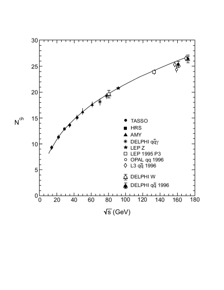
Figure 2: Mean charge particle multiplicity in $e^{+}e^{-}$ annihilation as function of total energy compared with the MLLA prediction. The data at energies $\geq M_{Z}$ have been corrected for increased multiplicity from $b$ and $c$ decays. $\!{}^{{\bf?}}$

The agreement with the data is generally good. As an example we show data in the range from 20 to 180 GeV in Fig. 2. $\!{}^{{\bf?}}$ The curve represents Eq. (42) where ${\mathcal{N}}$ is multiplied with $(1+d\sqrt{\alpha_{s}})$ to allow for the possibility of a next-to-next-to-leading-order correction. Fitted parameters are the overall normalization, $\alpha_{s}(m_{Z})=0.119\pm 0.003$ and $d=1.11\pm 0.39$. Recent measurements at LEP-2 $\!{}^{{\bf?}}$ follow the extrapolation from lower energies although they are systematically a bit at the low side. For example, the fit to data between 12 and 161 GeV predicts ${\mathcal{N}}_{ch}=27.6$ at 189 GeV which is to be compared with the measurement $\!{}^{{\bf?}}$ ${\mathcal{N}}_{ch}=26.95$ $\pm$ 0.16(stat.) $\pm$ 0.51(syst.). Recently a comparison of data with the prediction including the higher order terms up to 3NLO has been performed. $\!{}^{{\bf?}}$ Fitting the normalization and the coupling leads to a good result with reasonable $\Lambda$ in the range 0.12-0.26 GeV.

Figure 3: Data on the average jet multiplicity ${\mathcal{N}}$ at $Q$ = 91 GeV for different resolution parameters $y_{c}$ (lower set) and the average hadron multiplicity (assuming ${\mathcal{N}}=\frac{3}{2}{\mathcal{N}}_{ch}$) at different $cms$ energies between $Q=3$ and $Q=91$ GeV using $Q_{c}=Q_{0}$ = 0.508 GeV in the parameter $y_{c}$ (upper set). The curves follow from the evolution equation (36) with $\Lambda$ = 0.5 GeV; the upper curve for hadrons is based on the duality picture (34) with $K=1$ and parameter $\lambda=\ln(Q_{0}/\Lambda)=0.015$ (Figure from Ref. 74).

Figure 4: Jet multiplicities extending towards lower $y_{cut}$ parameters; full lines as in Fig. 3 for jets, dashed lines the same predictions but shifted $y_{cut}\to y_{cut}-Q_{0}^{2}/Q^{2}$ according to the different kinematical boundaries as in (35), with parameters as in Fig. 3 (data from OPAL $\!{}^{{\bf?},{\bf?}}$).

Alternatively, one can compare the data with predictions from the full parton cascade using the normalization at threshold. The numerical solution of the pair of evolution equations (36) with (38) has been compared with data on $e^{+}e^{-}$ annihilation; in this calculation the term of order $\alpha_{s}$ had been replaced by the result from the full matrix element of the same order. $\!{}^{{\bf?}}$ The predictions from this analysis for both, jets and hadrons, are shown in Fig. 3 together with the data.

The lower set of data refers to the jet multiplicity at variable resolution $y_{cut}=(Q_{c}/Q)^{2}$ calculated at fixed total energy $Q$. For $y_{cut}\to 1$ all particles are combined into two jets and therefore ${\mathcal{N}}\to 2$ as discussed in (4). On the other hand, for $y_{cut}\to 0$ all hadrons are resolved and ${\mathcal{N}}\to{\mathcal{N}}_{had}$. The theoretical prediction describes the data reasonably well down to $y_{cut}\sim 10^{-4}$ and is determined fully by the parameter $\Lambda$.

An improvement of the description for large $y_{cut}$ is possible if 2-loop results are used. For $y_{cut}\mathrel{\mathop{\kern 0.0pt\hbox to0.0pt{\raise 0.86108pt\hbox{$>$}\hss}}\lower 3.87495pt\hbox{\kern-1.90002pt$\sim$}}0.01$ the data are well described by the complete matrix element calculations to $O(\alpha_{s}^{2})$. In the region $y_{cut}\mathrel{\mathop{\kern 0.0pt\hbox to0.0pt{\raise 0.86108pt\hbox{$>$}\hss}}\lower 3.87495pt\hbox{\kern-1.90002pt$\sim$}}10^{-3}$ the resummation of the higher orders in $\alpha_{s}$ is important. $\!{}^{{\bf?}}$ The calculation at large $y_{cut}$ allows the precise determination of the coupling or, equivalently, of the QCD scale parameter $\Lambda_{\overline{MS}}$.  $\!{}^{{\bf?},{\bf?}}$

The multiplicity diverges for small cut-off $Q_{cut}\to\Lambda$ as in this case the coupling $\alpha_{s}(k_{T})$ diverges. The divergence is shielded by the cut-off $Q_{0}$ and according to the duality picture in (34) the parton multiplicity represents the hadron multiplicity at this scale. It is found from the data that this happens for $Q_{c}=Q_{0}\simeq 0.5$ GeV if the total hadron multiplicity is taken as 3/2 of the charged multiplicity. The corresponding calculation at lower $cms$ energies is in agreement with the hadron multiplicity data down to $Q=3$ GeV with the same parameter $Q_{0}$ as shown by the upper set of data and the theoretical curve in Fig. 3. Interestingly, the normalization constant in (34) can be chosen as

$$K\approx 1,$$ (57)

whereas in previous approximate calculations using the limiting spectrum (55) the value $K\approx 2$ has been obtained. $\!{}^{{\bf?}}$ The parameter $K$ is correlated with $Q_{0}$ and can be varied within about 30%. The result $K=1$ implies that the hadrons, in the duality picture, can be viewed as very narrow jets with low resolution parameter $Q_{0}\sim$ a few 100 MeV.

The behavior of multiplicities in Fig. 3 is close to the qualitative expectations from the DLA discussed in Sect. 3.2. The running of the coupling $\alpha_{s}$ is crucial for the results. Namely, for constant $\alpha_{s}$ both curves for hadrons and jets would coincide and follow a power law in the ratio of available scales $Q_{cut}/Q$ as in (48). With running $\alpha_{s}(k_{T}/\Lambda)$ the absolute scale of $Q_{cut}$ matters: $\alpha_{s}$ varies most strongly for $Q_{cut}\to\Lambda$ for jets at small $y_{cut}$ and for hadrons near the threshold of the process at large $y_{cut}$ (small $Q$) where again $\alpha_{s}\mathrel{\mathop{\kern 0.0pt\hbox to0.0pt{\raise 0.86108pt\hbox{$>$}\hss}}\lower 3.87495pt\hbox{\kern-1.90002pt$\sim$}}1$.

Recently, data became available at smaller $y_{cut}$ in a wide energy range from 35 to 183 GeV $\!{}^{{\bf?},{\bf?}}$ and examples are shown in Fig. 4. In the theoretical calculation all hadrons are resolved for $Q_{cut}\to Q_{0}$ whereas in the experimental quantities this happens for $Q_{cut}\to 0$. This kinematical mismatch can be avoided $\!{}^{{\bf?}}$ by a shift in $y_{cut}$ according to (35). The shifted (dashed) curves in Fig. 4 describe the data rather well whereby the $Q_{0}$ parameter has been taken from the fit to the hadron multiplicity before; the predictions fall a bit below the data at the lower energies like 35 GeV. The non-perturbative $Q_{0}$ correction becomes negligible for $Q_{c}>1.5$

It appears that the final stage of hadronization in the jet evolution can be well represented by the parton cascade with small cut-off $Q_{0}$ and with the standard 1-loop running coupling. This description clearly goes beyond standard perturbation theory which is determined entirely by the QCD scale $\Lambda$. The calculation in the soft region rather corresponds to a non-perturbative model which involves a hadronization scale $Q_{0}$. In some kinematic regions (small $k_{\perp}$) the coupling becomes large $\alpha_{s}/\pi\sim{\cal O}(1)$ but – as experienced with the analytical DLA results – there is good convergence of the leading log summation also in this region as the higher order terms are suppressed by soft gluon coherence effects.

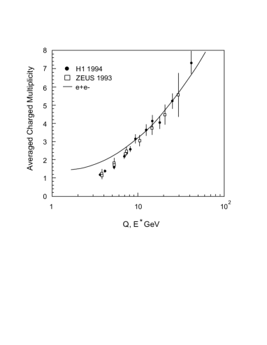
Figure 5: Average charged particle multiplicity in the current fragmentation region of the Breit frame as measured by H1 and ZEUS Collaborations at momentum transfer $Q$ in comparison with $e^{+}e^{-}$ results at $cms$ energy $E^{*}=Q$. $\!{}^{{\bf?}}$

3.6 Test of Jet Universality

Results on quark jet fragmentation are expected to be universal in the parton model. $\!{}^{{\bf?}}$ If we consider the particle multiplicity the soft particles are included and in this case the reference frame becomes important. In deep inelastic lepton proton scattering at momentum transfer $Q^{2}$ the particles in the current fragmentation region in the Breit frame should be compared with the multiplicity of one hemisphere in $e^{+}e^{-}$ collisions at $cms$ energy $E^{*}=Q$ (see, for example, Refs. 1,82-84) Results of such a comparison are shown in Fig. 5. The DIS results approach those from $e^{+}e^{-}$ for energies $Q\mathrel{\mathop{\kern 0.0pt\hbox to0.0pt{\raise 0.86108pt\hbox{$>$}\hss}}\lower 3.87495pt\hbox{\kern-1.90002pt$\sim$}}10$ GeV. At lower energies processes not available in $e^{+}e^{-}$ annihilation like photon gluon fusion are important. The agreement at higher energies confirms the universality of the jet fragmentation and the relevance of the Breit frame.

3.7 Comparison of Quark and Gluon Jets

The experimental results on multiplicities in quark jets are derived as half of the total multiplicity of $e^{+}e^{-}$ annihilation or the multiplicity in the current region of DIS. These experimental results are well met by the perturbative calculations (and their non-perturbative extensions).

The situation is more difficult for gluon jets and the following results have been presented:

1. A fully inclusive measurement is possible at lower energies $Q$ from radiative decays of $\Upsilon(1S)$ which are assumed to proceed in lowest perturbative order through $\Upsilon\to\gamma gg$. This yields measurements at $Q\sim 5$ GeV of the $gg$ system. $\!{}^{{\bf?}}$ Similarly, results have been obtained near 10 GeV from the decay $\Upsilon(3S)\to\gamma\chi_{b2}$, $\!{}^{{\bf?}}$ assuming $\chi_{b2}\to gg$. At $Q\sim 5$ GeV the ratio $r$ is still compatible with unity.

2. At higher energies the multiplicities have to be extracted from gluon jets in a more complex multi-jet environment, either 3-jet events in $e^{+}e^{-}$ or high $p_{T}$ jets in $pp$ colliders. A simple situation is met again in $e^{+}e^{-}\to$ 3 jets with two quark jets (taken as identified $b$ quark jets) recoiling together against the gluon. This possibility has been pointed out some time ago $\!{}^{{\bf?}}$ and worked out in detail for $e^{+}e^{-}$ annihilation. $\!{}^{{\bf?}}$ Results on the multiplicity in the gluon hemisphere have been obtained in this way by OPAL $\!{}^{{\bf?}}$ and the ratio $r$ is found to be $r=1.514\pm 0.019\pm 0.034$ at $Q\sim 80$ GeV.

3. Furthermore, results have been obtained from symmetric 3 jet events in Y-configuration with a quark in one hemisphere and quark and gluon in the other one. $\!{}^{{\bf?}}$ In this case the gluon jet multiplicity is obtained as difference of the 3 jet and the known $q\overline{q}$ multiplicity as suggested by a perturbative leading order analysis. $\!{}^{{\bf?},{\bf?}}$ The results obtained in the intermediate energy region interpolate between the $Q=10$ and $Q=80$ results above.

4. The ratio $r$ has also been determined from high $p_{T}$ jet production with dijet masses in the range 100-600 GeV at the TEVATRON by CDF. $\!{}^{{\bf?}}$ The energy dependence of the multiplicity has been assumed to follow the “limiting spectrum” formula (55). Using the known composition of quark and gluon jets the energy dependence of the multiplicity is then predicted for a given ratio $r$. The curves in Fig. 6, calculated for fixed ratios, are then compared to the data which yields the estimate $r=1.7\pm 0.3$ over this energy range.

The experimental results 1. and 2. do not use further theoretical input and have been compared with the asymptotic predictions and with the numerical solutions of the evolution equations; both are found not fully satisfactory.

1. In the first approach $\!{}^{{\bf?}}$ the 3NLO asymptotic expression is fit to the gluon jet data at $Q\sim 5,10$ and $80$ GeV by adjusting the normalization and $\Lambda$. Using the corresponding expression for $r={\mathcal{N}}_{g}/{\mathcal{N}}_{q}$ and taking the same parameters one can predict the multiplicity in quark jets. This is now found lower over the full energy region by 20-30%. Correspondingly the ratio $r$ is predicted larger than the measurements.

2. In the second approach $\!{}^{{\bf?}}$ the numerical solution of the evolution equations (36) is fit to the $e^{+}e^{-}$ data and the parameters $Q_{0}$ and $\Lambda$ are determined. The fits are found satisfactory (see Sect. 3.5). The gluon jet multiplicity from the same solution are now compared with data. There is a good agreement with the OPAL result at $Q\sim 80$ GeV but the prediction for CLEO at $Q\sim 5$ GeV is too large by 20%. It has been argued that at low energy the exact treatment of the ${\cal O}(\alpha_{s})$ term is important as was found explicitly for quark jets. For the gluon jets at the $\Upsilon$ such calculations have not been performed yet. Another explanation could be a large non-perturbative effect for gluons which “freezes” the gluon degrees of freedom at low energies. It is interesting to note that the result from the HERWIG Monte Carlo shows a similar behavior with too large ratio $r$ at low energies.

At higher energies the numerical solutions yield a rise from $r=1.54$ at $Q=100$ GeV to $r=1.68$ at $Q=600$ GeV which is consistent with the CDF result within the large error.

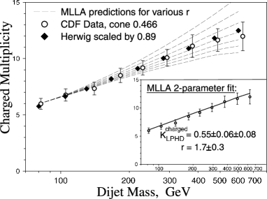
Figure 6: Charged multiplicity in a high $p_{T}$ jet with cone opening 0.466 rad for different dijet masses in comparison with MLLA predictions for different values of the ratio $r={\mathcal{N}}_{g}/{\mathcal{N}}_{q}$. The curves corresponds to $r=1.0,1.2,1.4,1.6,1.8,2.0,2.25$. $\!{}^{{\bf?}}$

Taking these results together there is a clear evidence for the difference of quark and gluon jet multiplicities. The ratio $r$ at presently accessible energies is much smaller than the asymptotic value $r=9/4$. It is a considerable success that at the higher LEP energies there is agreement with perturbative QCD calculations if all non-leading logarithmic terms from the MLLA evolution equation are included.

4 Momentum Spectra of Particles Inside Jets

We start from the MLLA evolution equation for particle spectra and consider solutions relevant for the small $x$ region. The early DLA results on the approximately Gaussian shape of the distribution (“hump-backed plateau”) $\!{}^{{\bf?},{\bf?}}$ in the variable

$$\xi=\ln\frac{1}{x_{p}},\qquad x_{p}=\frac{p}{E_{jet}},$$ (58)

for momentum $p$ of the particle has been an important milestone in the application of perturbative QCD to the multiparticle phenomena. They demonstrated the relevance of angular ordering and color coherence to the particle spectra at low momentum. The success of the improved calculations within MLLA accuracy gave strong support to the concept of LPHD. This Gaussian shape is found quite universally in jets from various collision processes and also for all particle species; however, the differences observed for various species is not yet quantitatively understood. We will discuss here some MLLA based computations and compare them with typical recent results from $e^{+}e^{-}$, $ep$ and $\overline{p}p$ colliders whereby we include some striking phenomena with the very soft particles ($\mathrel{\mathop{\kern 0.0pt\hbox to0.0pt{\raise 0.86108pt\hbox{$<$}\hss}}\lower 3.87495pt\hbox{\kern-1.90002pt$\sim$}}$ 1 GeV), as well as the energy evolution of spectra from threshold to asymptotic energies.

Whereas this analysis is focused on the small $x$ domain of the particle spectra there is a complementary approach which treats the evolution equation in the larger $x_{p}$ region (say, $x\mathrel{\mathop{\kern 0.0pt\hbox to0.0pt{\raise 0.86108pt\hbox{$>$}\hss}}\lower 3.87495pt\hbox{\kern-1.90002pt$\sim$}}0.1$) (“fragmentation function”) for which results in 2-loop accuracy for the running coupling are available. Such studies are an important tool for the determination of the strong coupling. $\!{}^{{\bf?},{\bf?},{\bf?}}$ This approach is expected to be more precise at large $x_{p}$ as compared to the 1-loop MLLA calculations, on the other hand it does not take into full account the contributions important for the soft region. Furthermore, in this approach an ansatz involving several parameters is required for the fragmentation function(s) at a particular finite energy whereas the MLLA/LPHD approach has only one essential non-perturbative parameter $Q_{0}$.

4.1 Evolution Equation for $\xi$-Spectra and Approximate Solutions

The inclusive distribution of partons $b$ in a jet from parton $a$ is obtained from the generating functional through

$$x{D}_{a}^{b}(x)=E_{b}\frac{\delta}{\delta u(k_{b})}Z_{a}(E_{a},\Theta;\{u\})|_{u=1}$$ (59)

and its evolution equation from Eq.(30). In the approximation $1-z\approx 1$ it takes the form

$$\frac{d}{dY}x{D}_{A}^{B}(x,Y)=\sum_{C=q,\overline{q},g}\int_{0}^{1}dz\frac{\alpha_{s}(k_{\perp})}{2\pi}\Phi_{A}^{C}(z)\left[\frac{x}{z}{D}_{C}^{B}\left(\frac{x}{z},Y+\ln z\right)\right],$$ (60)

where $Y=\ln(P\Theta/Q_{0})$ and $\Phi_{A}^{C}$ stands for the DGLAP splitting functions. The boundary condition for (60) reads

$$x{D}_{A}^{B}(x)|_{Y=0}=\delta(1-x)\delta_{A}^{B}.$$ (61)

The scale of the coupling is given by the transverse momentum taken as $k_{\perp}\simeq z(1-z)E\Theta$. The shower evolution is cut off by the parameter $Q_{0}$, such that $k_{\perp}\geq Q_{0}$ and this restriction is understood in (60).

The integral equation can be solved by Mellin transform

$$D_{\omega}(Y,\lambda)=\int_{0}^{1}\frac{dx}{x}x^{\omega}\left[x{D}(x,Y,\lambda)\right]=\int_{0}^{Y}d\xi e^{-\xi\omega}\>D(\xi,Y,\lambda).$$ (62)

In flavor space the valence quark and ($\pm$) mixtures of sea quarks and gluons evolve independently with different “eigenfrequencies” $\nu_{\pm}(\omega)$. At high energies and $x\ll 1$, the dominant contribution to the inclusive spectrum comes from the “plus”-term, which we denote by $D_{\omega}(Y,\lambda)\equiv D_{\omega}^{+}(Y,\lambda)$. In an approximation where only the leading singularity plus a constant term is kept $\nu_{+}(\omega)\approx 4N_{C}/\omega-a$, one obtains in a sequence of steps from (60) the following evolution equation $\!{}^{{\bf?}}$

$$\left(\omega+\frac{d}{dY}\right)\frac{d}{dY}D_{\omega}(Y,\lambda)-4N_{C}\frac{\alpha_{s}}{2\pi}D_{\omega}(Y,\lambda)=-a\left(\omega+\frac{d}{dY}\right)\frac{\alpha_{s}}{2\pi}D_{\omega}(Y,\lambda),$$ (63)

where

$$a=\frac{11}{3}N_{C}+\frac{2n_{f}}{3N_{C}^{2}}.$$ (64)

and the boundary condition corresponding to (61) is $D_{\omega}(0,\lambda)=1$. Restricting to the leading term by setting $a=0$, i.e. dropping the $r.h.s.$ in (63), yields the DLA evolution equation. One can now derive asymptotic solutions at high energies in leading-order and next-to-leading order or a full solution of the evolution equation (63) including the boundary condition at threshold.

Introducing the anomalous dimension $\gamma_{\omega}$ according to

$$D_{\omega}(Y,\lambda)=D_{\omega}(Y_{0},\lambda)\exp\left(\int_{Y_{0}}^{Y}dy\gamma_{\omega}\left[\alpha_{s}(y)\right]\right),$$ (65)

the evolution equation (63) can be expressed in terms of a differential equation for $\gamma_{\omega}$

$$(\omega+\gamma_{\omega})\gamma_{\omega}-\frac{4N_{C}\alpha_{s}}{2\pi}=-\beta(\alpha_{s})\frac{d}{d\alpha_{s}}\gamma_{\omega}-a(\omega+\gamma_{\omega})\frac{\alpha_{s}}{2\pi},$$ (66)

where $\beta(\alpha_{s})=\frac{d}{dY}\>\alpha_{s}(Y)\simeq-b\>\frac{\alpha_{s}^{2}}{2\pi}$. For the DLA one finds

$$(\omega+\gamma_{\omega})\gamma_{\omega}-\gamma_{0}^{2}=0,\quad\gamma_{\omega}^{DLA}(\alpha_{s})=\frac{1}{2}\left(-\omega+\sqrt{\omega^{2}+4\gamma_{0}^{2}}\right);$$ (67)

with

$$\gamma_{0}^{2}=\gamma_{0}^{2}(\alpha_{s})\equiv 2N_{C}\frac{\alpha_{s}}{\pi}.$$ (68)

Choosing the (+) sign for the square root yields the solution which dominates at high energies whereas the solution with the (–) sign would die out.

The next-to-leading order result in MLLA follows from Eq. (66) including the $r.h.s.$ where the first term proportional to the $\beta$-function keeps trace of the running coupling effects while the second accounts for the hard corrections to the soft singularities in the splitting function. In comparison to the leading term they are of relative order $\sqrt{\alpha_{s}}$ and the MLLA correction to DLA reads

$$\gamma_{\omega}\;=\;\gamma^{DLA}_{\omega}\>+\>\frac{\alpha_{s}}{2\pi}\>\left[-\frac{a}{2}\>\left(1+\frac{\omega}{\sqrt{\omega^{2}+4\gamma_{0}^{2}}}\right)\>+\>b\frac{\gamma_{0}^{2}}{\omega^{2}+4\gamma_{0}^{2}}\right]\>+\>O(\alpha_{s}^{3/2}).$$ (69)

Instead of these asymptotic solutions one can also find directly an analytical expression for the exact solution of the differential equation (63) in terms of confluent hypergeometric functions  $\!{}^{{\bf?},{\bf?}}$

$$D_{\omega}(Y,\lambda) = \frac{\Gamma(A+1)}{\Gamma(B+2)}z_{1}z_{2}^{B}\{\Phi(-A+B+1,B+2,-z_{1})\Psi(A,B+1,z_{2})$$

$$+ e^{z_{2}-z_{1}}(B+1)\Psi(A+1,B+2,z_{1})\Phi(-A+B+1,B+1,-z_{2})\},$$

where we have used the notation

$$A=\frac{4N_{C}}{b\omega},\quad B=\frac{a}{b},\qquad z_{1}=\omega(Y+\lambda),\quad z_{2}=\omega\lambda.$$ (71)

From these representations of $D_{\omega}$ one can reconstruct the $x$ (or $\xi$) distributions by inverse Mellin transformation

$$\left[x{D}(x,Y,\lambda)\right]\equiv{D}(\xi,Y,\lambda)=\int_{\epsilon-i\infty}^{\epsilon+i\infty}\frac{d\omega}{2\pi i}x^{-\omega}D(\omega,Y,\lambda)$$ (72)

where the integral runs parallel to the imaginary axis to the right of all singularities of the integrand in the complex $\omega$-plane.

4.2 Moments

It is convenient to analyze the properties of the $\xi$ spectrum in greater detail in terms of the normalized moments $\!{}^{{\bf?},{\bf?}}$

$$\xi_{q}\equiv<\xi^{q}>=\frac{1}{{\mathcal{N}}}\int d\xi\xi^{q}D(\xi).$$ (73)

Also one defines the cumulant moments $K_{q}$ or the reduced cumulants $k_{q}\equiv K_{q}/\sigma^{q}$, which are given for $q\leq 4$ by

$$K_{1} \equiv \overline{\xi}\;\equiv\;\xi_{1}$$

$$K_{2} \equiv \sigma^{2}\;=\;<(\xi-\overline{\xi})^{2}>,$$

$$K_{3} \equiv s\sigma^{3}\;\equiv\;<(\xi-\overline{\xi})^{3}>,$$

$$K_{4} \equiv k\sigma^{4}\;\equiv\;<(\xi-\overline{\xi})^{4}>\>-\>3\sigma^{4},$$ (74)

where the third and forth reduced cumulant moments are the skewness $s$ and the kurtosis $k$ of the distribution.

The cumulant moments can be found using the expansion of the Mellin-transformed spectrum $D_{\omega}(Y,\lambda)$ in (62):

$$\ln\>D_{\omega}(Y,\lambda)\;=\;\sum_{q=0}^{\infty}\;K_{q}(Y,\lambda)\;\frac{(-\omega)^{q}}{q!}.$$ (75)

The high energy behavior of moments in next-to-leading order can be obtained with $K_{q}(Y,\lambda)=\left.(-\partial/\partial\omega)^{q}\ln D_{\omega}(Y,\lambda)\right|_{\omega=0}$. From the high energy approximation of the anomalous dimension $\gamma_{\omega}$ in (69) using (65)

$$K_{q}=\int_{0}^{Y}dy\left.\left(-\frac{\partial}{\partial\omega}\right)^{q}\gamma_{\omega}(\alpha_{s}(y))\right|_{\omega=0},$$ (76)

which shows the direct dependence of the moments on $\alpha_{s}(Y)$. For fixed $\alpha_{s}$, for example, one obtains simply $K_{q}(Y)\propto Y$ for high energies. Alternatively, one can derive evolution equation for the moments $\!{}^{{\bf?}}$ and derive the high energy behavior in next-to-leading order. Approximate forms for the yet higher order terms can be obtained from Eq. (LABEL:2.34) for arbitrary $\lambda$ and in particular for the limiting spectrum with $\lambda=0$.

The mean of the $\xi$ distribution in MLLA proves to have an energy dependence of the form $\!{}^{{\bf?},{\bf?},{\bf?}}$

$$\overline{\xi}=Y\left[\frac{1}{2}+\sqrt{\frac{C}{Y}}+\frac{\overline{a}}{Y}+\overline{b}Y^{-3/2}\right]$$ (77)

with

$$C=\frac{a^{2}}{16N_{C}b}=0.2915(0.3513)\;{\rm for}\;n_{f}=3(5).$$ (78)

The moments evolve in different energy regions according to the relevant number of flavors $n_{f}$. It turns out that even at the energies of LEP-2 the approximation $n_{f}=3$ is rather good, in any case better than $n_{f}=5$. $\!{}^{{\bf?},{\bf?}}$

A quantity closely related to $\overline{\xi}$ is the position of the maximum $\xi^{*}$ which differs from $\overline{\xi}$ only in higher order terms $\overline{a},\overline{b}$ in (77). For the limiting spectrum one finds $\!{}^{{\bf?},{\bf?},{\bf?}}$

$$\xi^{*}=Y\left[\frac{1}{2}\>+\>\sqrt{\frac{C}{Y}}\>-\>\frac{C}{Y}\right].$$ (79)

This form leads to a nearly linear dependence of $\xi^{*}$ on $Y$. It is worthwhile to mention that in the large $N_{C}$ limit, when $11N_{C}\gg 2n_{f}$ (cf. Eqs.(5) and (64)) the parameter $C$ becomes independent on both $n_{f}$ and $N_{C}$ and approaches its asymptotic value of $C=\frac{11}{3}\frac{1}{2^{4}}\simeq 0.23$. Therefore in this limit the effective gradient of the straight line is determined by such a fundamental parameter of QCD as the celebrated $\frac{11}{3}$ factor (characterizing the gluon self interaction) in the coefficient $b$.

The shape parameters $\sigma,k,s$ for the limiting spectrum have been derived in next-to-leading order at $N_{C}=3$ as

$$\sigma = \frac{Y}{\sqrt{3z}}\;\left(1\>-\>\frac{3}{4z}\right)\;+\;O(Y^{-1/4})$$ (80)

$$s = -\>\frac{a}{16}\;\frac{1}{\sigma}\;+\;O(Y^{-3/4})$$ (81)

$$k = -\>\frac{27}{5Y}\;\left(\frac{Y}{\sqrt{z}}\;-\;\frac{b}{24}\right)\;+\;O(Y^{-3/2})$$ (82)

where $z=\sqrt{16N_{C}Y/b}$. It is worthwhile to notice that the next-to-leading effects are very substantial at present energies. In particular, the spectrum significantly softens because of energy conservation effects. This influences the rate of particle multiplication which is strongly overestimated by the DL approximation.

The asymptotic behavior $(n\geq 1)$ can be obtained from (76) with (69)

$$\sigma^{2} \sim Y^{3/2}$$ (83)

$$k_{2n+2} \sim \left(\sqrt{Y}\right)^{-n}$$ (84)

$$k_{2n+1} \sim \left(\sqrt{Y}\right)^{-n-1/2}.$$ (85)

One concludes that the higher cumulants $(n>4)$ appear to be less significant for the shape of the spectrum in the hump region $\delta\lower 3.01385pt\hbox{$\;\stackrel{{\scriptstyle\textstyle<}}{{\sim}}\;$}1$.

The higher order terms in the series expansion (80-82) left out are still numerically sizable at LEP-1 energies  $\!{}^{{\bf?}}$ ($\sim$ 10% contribution from next-to-MLLA corrections to $\bar{\xi}$ and $\sigma^{2}$) and increase towards lower energies. Therefore, it is appropriate in a comparison with the data over a larger energy interval to use the full result from the MLLA solution (LABEL:2.34) including the boundary condition (61). A further discussion of the higher moments is found in the review. $\!{}^{{\bf?}}$

4.3 Predictions for the $\xi$-Spectra

Next we present analytical results for some interesting limits.

• Asymptotic Gaussian

The simplest example is the DLA prediction which corresponds to the spectrum at very high energies. Near the maximum one finds an approximately Gaussian shape $\!{}^{{\bf?},{\bf?}}$

$$D(\xi,Y)\simeq\frac{{\mathcal{N}}(Y)}{\sqrt{2\pi\sigma^{2}}}\exp\left(-\frac{1}{2}\delta^{2}\right)$$ (86)

where

$$\delta=\frac{(\xi-\overline{\xi})}{\sigma},\qquad\overline{\xi}=\frac{Y}{2},\qquad\sigma^{2}=\frac{(Y+\lambda)^{3/2}-\lambda^{3/2}}{12(N_{C}/b)^{1/2}}$$ (87)

with multiplicity ${\mathcal{N}}(Y)\sim\exp(\sqrt{16N_{C}(Y+\lambda)/b})$ at high energies as in (50). This approximately Gaussian shape (“hump-backed plateau”) is an important prediction of QCD. The drop of the spectrum towards small momenta (large $\xi$) is a consequence of the coherent emission of soft gluons from the faster ones in the jet and we will come back to this phenomenon in more detail below.

• Limiting Spectrum

In perturbation theory one is usually restricted to regions where $\alpha_{s}$ is small, this would require $\lambda\gg 1$. However, one can see that in Eq. (86) the shape has a smooth limit for $\lambda\to 0$, i.e. $\alpha_{s}\to\infty$. Therefore, the shape is in this sense infrared safe.

In this limit $\lambda\to 0$ one can derive an analytic expression for the $\xi$ spectrum from the full MLLA equation (LABEL:2.34) using an integral representation for the hypergeometric function $\Phi$, $\!{}^{{\bf?},{\bf?},{\bf?}}$

$${D}^{\lim}(\xi,Y) = \frac{4N_{C}}{b}\>\Gamma(B)\;\int_{-\frac{\pi}{2}}^{\frac{\pi}{2}}\;\frac{d\ell}{\pi}\>e^{-B\alpha}\;\left[\frac{\cosh\>\alpha+(1-2\zeta)\sin h\>\alpha}{\frac{4N_{C}}{b}\;Y\;\frac{\alpha}{\sinh\>\alpha}}\right]^{B/2}$$ (88)

$$\times\;I_{B}\;\left(\sqrt{\frac{16N_{C}}{b}\;Y\;\frac{\alpha}{\sinh\>\alpha}\;[\cosh\>\alpha+(1-2\zeta)\>\sinh\>\alpha]}\right).$$

Here $\alpha=\alpha_{0}+i\ell$ and $\alpha_{0}$ is determined by $\tanh\>\alpha_{0}=2\zeta-1$ with $\zeta=1-\frac{\xi}{Y}$. $I_{B}$ is the modified Bessel function of order $B$. In the present approximation this distribution describes the gluon spectrum in a gluon jet. For the quark jet this distribution is to be multiplied by $C_{F}/N_{C}=4/9$. The spectrum (88) reproduces the Gaussian behavior near the maximum.

There is one caveat on the distribution (88). As pointed out in Sect. 3.2 the multiplicity ${\mathcal{N}}\sim\int D(\xi)d\xi$ diverges logarithmically for $\lambda\to 0$. In the MLLA evolution equation the terms beyond next-to-leading order in the $\sqrt{\alpha_{s}}$ expansions are dropped which is justified for small $\alpha_{s}$. The gluon emission near threshold at $\xi\sim Y$ (small momentum $p\sim Q_{0}$) involves large $\alpha_{s}$ and is therefore not expected to be well approximated in (88).

• Distorted Gaussian

The spectrum near the maximum can be represented by a distorted Gaussian distribution and one finds for small $\delta\mathrel{\mathop{\kern 0.0pt\hbox to0.0pt{\raise 0.86108pt\hbox{$<$}\hss}}\lower 3.87495pt\hbox{\kern-1.90002pt$\sim$}}1$ in terms of the cumulant moments $\!{}^{{\bf?}}$

$${D}(\xi)\simeq\frac{{\mathcal{N}}}{\sigma\sqrt{2\pi}}\exp\left[\frac{1}{8}k-\frac{1}{2}s\delta-\frac{1}{4}(2+k)\delta^{2}+\frac{1}{6}s\delta^{3}+\frac{1}{24}k\delta^{4}\right].$$ (89)

Relative to the leading-order predictions, the moments in MLLA accuracy (80)-(82) imply that the peak in the $\xi$-distribution is shifted up (i.e. to lower $x$), narrowed, skewed towards lower $\xi$, and flattened, with tails that fall off more rapidly than a Gaussian.

Figure 7: Spectrum in $\xi=\ln(1/x)$ as obtained from the MC calculation for a parton cascade including the soft gluon coherence which shows the approximately Gaussian shape. Also shown is the spectrum for a cascade without coherence. $\!{}^{{\bf?}}$

• Numerical results

The evolution of the parton jet in its probabilistic approximation but taking into account soft gluon interference can also be treated numerically with Monte Carlo methods. In Fig. 7 we show the $\xi$ spectrum for $e^{+}e^{-}$ annihilation at energy $Q=100$ GeV as obtained from the Marchesini-Webber $\!{}^{{\bf?}}$ MC which includes coherence in the soft gluon radiation. One can clearly see the typically Gaussian shape. On the other hand, if the coherence is “switched off” in the MC the distribution looses its Gaussian shape and instead peaks near the edge of phase space for the soft particles ($\xi\mathrel{\mathop{\kern 0.0pt\hbox to0.0pt{\raise 0.86108pt\hbox{$<$}\hss}}\lower 3.87495pt\hbox{\kern-1.90002pt$\sim$}}Y$, $p\mathrel{\mathop{\kern 0.0pt\hbox to0.0pt{\raise 0.86108pt\hbox{$>$}\hss}}\lower 3.87495pt\hbox{\kern-1.90002pt$\sim$}}Q_{0}$).

• The Soft Limit of the Particle Spectrum

In this limit the coherence of the soft gluon emission plays an important role. If a soft gluon is emitted from a $q\overline{q}$ two-jet system then it cannot resolve with its large wave length all individual partons but only “sees” the total charge of the primary partons $q\overline{q}$. In the analytical treatment, this property follows from the dominance of the Born term of ${\cal O}(\alpha_{s})$ and one expects a nearly energy independent spectrum. $\!{}^{{\bf?}}$

This property has been studied recently in greater detail. $\!{}^{{\bf?},{\bf?}}$ An analytical formula applicable for the low momenta $p$ and $p_{T}$ has been given and its general behaviour reads

$$\frac{dn}{dydp_{T}^{2}}\ \sim\ C_{A,F}\frac{\alpha_{s}(p_{T})}{p_{T}^{2}}\left(1+{\cal O}\left(\ln\frac{\ln(p_{T}/\Lambda)}{\ln(Q_{0}/\Lambda)}\ \ln\frac{\ln(p_{T}/(x\Lambda))}{\ln(p_{T}/\Lambda)}\right)\right)$$ (90)

for rapidity $y$ and momentum fraction $x$ where the second term is known within MLLA and vanishes for $p_{T}\to Q_{0}$. In this way the energy independence of the spectrum follows in the soft limit.

A crucial prediction $\!{}^{{\bf?}}$ from this approach is the dependence of the soft particle density on the color of the primary partons in (90): In the soft limit the particle density in gluon and quark jets should approach the ratio

$$R(g/q)\to\frac{C_{A}}{C_{F}}=\frac{9}{4}\qquad{\rm for}\qquad p_{T}\to Q_{0}$$ (91)

i.e. for the minimal $p_{T}$ or $p$. As discussed above, the prediction (91) has been obtained in the DLA for the total multiplicities at asymptotic energies. For the soft particles it is expected already at finite energies! The consequences have been worked out also for soft particle production in DIS and hadron hadron collisions. $\!{}^{{\bf?}}$ Further results on the soft particle production are discussed in a recent review. $\!{}^{{\bf?}}$

4.4 Comparison with Experimental Data

We begin with a discussion of the $\xi$ spectra. The observation of the Gaussian shape of these spectra and a good agreement with MLLA predictions in the PETRA energy range was a first success of the LPHD concept. $\!{}^{{\bf?}}$ The approximately Gaussian shape is confirmed in the meantime for the spectra in jets in the full variety of the hard collisions studied and also for different particle species. In general, the limiting spectrum provides a fairly good description of the data. We emphasize a few recent results:

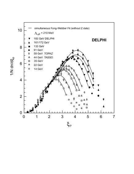
Figure 8: Distribution in $\xi_{p}=\ln(1/x_{p})$ for charged particles in $e^{+}e^{-}\to$ hadrons. The full lines represent the result of the simultaneous distorted Gaussian fit to all energies using moments within MLLA accuracy $\!{}^{{\bf?}}$ as performed by the DELPHI Collaboration. $\!{}^{{\bf?}}$

In $e^{+}e^{-}$ annihilations the study of spectra has been continued towards the higher energies of LEP-2. The DELPHI Collaboration $\!{}^{{\bf?}}$ has fitted the distorted Gaussian parametrization (89) to their data up to 183 GeV and those at lower energies $\!{}^{{\bf?},{\bf?}}$ down to 14 GeV using the moments in next-to-leading order (77,80-82). The fit has been performed to the central region where the distribution was larger than 60% of maximum height. The fitted parameters are $\Lambda=210\pm 8$ MeV, the constant $\overline{a}$ in (77) and the normalization using $n_{f}=3$. As can be seen from Fig. 8 the shape of the hump at the different energies is rather well described.

The limiting spectrum typically fits in a broader $\xi$ range and gives a good description of the spectra up to the LEP-1 $\!{}^{{\bf?}}$, also to LEP-1.5 $\!{}^{{\bf?}}$; the recent result from OPAL $\!{}^{{\bf?}}$ at 189 GeV indicates a slightly broader distribution (about 10% larger width) than expected from the extrapolation of lower energies.

Figure 9: Inclusive $\xi$ spectrum for charged particles in different jet opening cones fitted to the limiting spectrum in MLLA at the dijet mass of 378 GeV as measured by the CDF collaboration. $\!{}^{{\bf?}}$

Jets with high transverse energies $E_{T}$ from 40 to 300 GeV in $p\overline{p}$ collisions have been investigated by the CDF Collaboration $\!{}^{{\bf?}}$ at the TEVATRON whereby also the jet opening angle $\Theta$ has been varied between $\Theta=0.168$ and $\Theta=0.466$. The fitted value for $\Lambda=Q_{0}$ in the limiting spectrum was found rather stable $Q_{0}=240\pm 40$ MeV for the 45 data sets (5 cones $\times$ 9 dijet mass cuts). As an example, the evolution of the spectrum with the jet opening angle is shown in Fig. 9. The curves are seen to represent the data well within a few %. Similar results are obtained at other energies whereby the $\xi$ range of the successful fit increases with jet energy and opening angle.

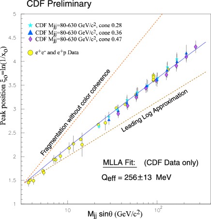
Figure 10: Peak position $\xi^{*}$ of the inclusive $\xi$ distribution plotted against di-jet mass $\times$ $\sin(\Theta)$ in comparison with the MLLA prediction (central curve); also shown are the double logarithmic approximation (lower curve with asymptotic slope $\xi^{*}\sim Y/2$) and expectation from cascade without coherence. Result by CDF Collaboration. $\!{}^{{\bf?}}$

A comparison of the peak position $\xi^{*}$ for the various jet energies and opening angles is shown in Fig. 10. The spectra depend on the evolution variable $Y=\ln(P\Theta/Q_{0})$ for small angle; a comparison is also performed with data at full angle $\Theta=\pi/2$ from $e^{+}e^{-}$ and $ep$ collisions whereby the variable $Y=\ln(P\sin\Theta/Q_{0})$ has been used. The data scatter around the expected curve (79) for $n_{f}=3$. Taking instead the scaling variable $Y=\ln(2P\sin(\Theta/2)/Q_{0})$ the full angle data would be shifted to the right by a factor $2\sin(\pi/4)\sim 1.4$. This would correspond essentially to a change of the next-to-next-to-leading order term in (79) but would not change the slope.

The slope is nicely confirmed and the leading DLA contribution ($\xi^{*}\sim Y/2$) is shown for comparison as the lower curve in Fig. 10, adjusted in height; the upper curve represents the spectrum for the incoherent cascade which peaks near the maximum ($\xi^{*}\sim Y)$. Apparently the data support the prediction from the parton cascade with suppression of soft particles due to coherent gluon emission in a large energy range $2E_{jet}\sin\Theta\sim~{}4-300$ GeV.

The analytical results for the particle spectrum near the soft limit (90) are nicely confirmed by the data. In these calculations the model (35) for mass effects has been used. The experimental data from the available range of energies in $e^{+}e^{-}$ annihilation ($Q=3-183$ GeV) and Deep Inelastic Scattering ($Q<20$ GeV) $\!{}^{{\bf?},{\bf?},{\bf?},{\bf?}}$ are well described by the calculations. The data are consistent with approaching the energy independent limit for small momenta $p\to 0$ and this conclusion does not depend on choosing a particular model for the mass effects.

It is more difficult to test prediction (91) as a $gg$ system is not easily available. From the study of 3-jet events in $e^{+}e^{-}$ annihilation with the gluon recoiling against a $q\overline{q}$ jet pair an estimate of this ratio of the soft particle yield in gluon and quark jets can be obtained. $\!{}^{{\bf?}}$ It approaches $R(g/q)\sim 1.8$ for $p\mathrel{\mathop{\kern 0.0pt\hbox to0.0pt{\raise 0.86108pt\hbox{$<$}\hss}}\lower 3.87495pt\hbox{\kern-1.90002pt$\sim$}}1$ GeV which is above the global multiplicity ratio $\sim$ 1.5 in the quark and gluon jets but still below the ratio $C_{A}/C_{F}=9/4$. It is plausible that this difference is due to the finite angle between the quark jets, i.e. a deviation from exact collinearity. $\!{}^{{\bf?}}$ It will be interesting to study the radiation pattern in more detail. A first result from such studies will be discussed in Section 7.

5 Multiparton Correlations Inside Jets

5.1 The General Structure of n-Parton Angular Correlations

The angular ordering is one of the most characteristic features of the parton cascade, c.f. Sub-section 2.3. This basic property of the elementary emissions has a direct counterpart in the angular dependence of multiparton correlations. They were derived in the analytical form by solving corresponding evolution equations with the aid of the resolvent (Greens function) method. This led to the integral representations used also in the jet calculus approach. $\!{}^{{\bf?}}$ The remaining integrals can be solved in the limit of the strong angular ordering providing a closed form of many multiparton distributions. For example, the fully differential angular correlation function of two gluons in a jet $(\vec{P},\Theta)$ reads $\!{}^{{\bf?},{\bf?}}$

$$\Gamma^{(2)}(\Omega_{1},\Omega_{2}) = D^{(2)}(\Omega_{1},\Omega_{2})-D^{(1)}(\Omega_{1})D(\Omega_{2})$$ (92)

$$= \frac{\gamma_{0}^{2}}{2(4\pi)^{2}}\frac{1}{\vartheta_{12}^{2}}\left(\frac{E\vartheta_{12}}{Q_{0}}\right)^{2\gamma_{0}}\left(\frac{1}{\vartheta_{1}^{2}}\left(\frac{\vartheta_{1}}{\vartheta_{12}}\right)^{\gamma_{0}/2}\Theta(\vartheta_{1}-\vartheta_{12})\right.$$

$$+ \left.\frac{1}{\vartheta_{2}^{2}}\left(\frac{\vartheta_{2}}{\vartheta_{12}}\right)^{\gamma_{0}/2}\Theta(\vartheta_{2}-\vartheta_{12})\right),$$

where $\vartheta_{i}$ denotes the angle between the momentum of i-th final parton and the momentum of the initial parton $\vec{P}$ and $E=|\vec{P}|$. The two terms in (92) describe two possible ways to produce the final configuration, namely $P\rightarrow 1\rightarrow 2$ and $P\rightarrow 2\rightarrow 1$. The relative angle $\vartheta_{12}$ is always restricted by the previous emission angle, i.e. $\vartheta_{ij}<\vartheta_{i},i=1,2$, differently in both terms. The above result was derived as the high energy limit of the DLA with the constant $\alpha_{s}$. However the generic structure of Eq. (92) remains the same also in more quantitative approximations and for arbitrary number of partons. This is seen in the general DLA result for n-parton connected correlation function also in the running $\alpha_{s}\;$   case

$$\Gamma^{(n)}(\{\Omega\})\simeq\left({f\over 4\pi}\right)^{n}{1\over n}\sum_{i=1}^{n}{\gamma_{0}^{n\over 2}(E\vartheta_{i})\over\vartheta_{i}^{2}}\exp{\biggl{(}2\beta\omega(\epsilon_{i},n)\sqrt{\ln E\vartheta_{i}/\Lambda}\biggr{)}}F_{i}^{n}(\{\chi\})\/.$$ (93)

Again, all the relative angles are limited by the corresponding polar angles of previous emissions. Here $\epsilon_{i}=\ln(\vartheta_{i}/(\vartheta_{ij})_{{\rm min}})/\ln(E\vartheta_{i}/\Lambda)$ and $F_{i}^{n}(\{\chi\})$ is homogeneous of degree $p=-2(n-1)$ in the relative angles built from factors $1/\vartheta_{ij}^{2}$. Similarly to the two parton case, Eq. (92), the correlation is a sum of $n$ terms, the $i$-th term describing a configuration with the parton $i$ emitted from (connected to) the initial parton at the polar angle $\vartheta_{i}$. All other partons in such a configuration are either connected to $i$ (factor $\vartheta_{ij}^{-2}$) or among themselves (factor $\vartheta_{jl}^{-2}$). The function $\omega(\epsilon,n)$ is a particular feature of the running $\alpha_{s}\;$ and will be discussed later. For small $\epsilon$ (large angles) the simple power behavior analogous to Eq. (92) emerges.

The above power dependence of the connected correlations is another characteristic property of a QCD cascade. From a simple picture of a branching process one may expect that the resulting parton distributions have a self similar, fractal structure. Indeed, Eq. (92) proves that such expectations are correct — QCD cascade is strictly self similar for constant $\alpha_{s}\;$ case. The evolution of a QCD cascade can be also easily visualized in a fractal phase space which has been constructed within the LUND dipole cascade model $\!{}^{{\bf?}}$. The Rényi dimension  of the inclusive n-parton configuration has been derived in Refs. 109,111,113,114 as

$$D_{n}={n+1\over n}\gamma_{0}.$$ (94)

On the other hand, the running $\alpha_{s}\;$ introduces a scale in the problem, hence the self similarity is only approximate.

Dynamics of QCD provides then a unique prediction for the structure of the multiparton correlation. This distinguishes between various phenomenological models $\!{}^{{\bf?}}$ of multiparticle production. In fact the way how the n-body correlation emerges from the two-body ones is very similar to the model of Van Hove proposed ten years ago. $\!{}^{{\bf?}}$

5.2 Distribution over the Relative Angle - Comparison with the Experiment

Predictions of the type of Eq. (92) allow to test the Local Parton Hadron Duality on a more differential, hence more detailed level. However full multibody correlations of higher order are notoriously difficult to measure experimentally. Nevertheless the measurements of particular sections of the two-body correlations inside a jet already exist and provide important checks of the theory. The distribution over the relative angle $\vartheta_{12}$ is such an object, hence we will discuss it in more detail. Consider two partons inside a jet $(\vec{P},\Theta),E=|\vec{P}|$ at fixed relative angle $\vartheta_{12}$. The density of $\vartheta_{12}$ has been calculated in various approximations. In the simplest case (same as in Eq.(92)) it reads

$${dN^{(2)}\over d\vartheta_{12}} \equiv \int D^{(2)}(\Omega_{1},\Omega_{2})\delta(\vartheta_{12}-\Theta_{12})$$ (95)

$$= {\gamma_{0}\over 2\vartheta_{12}}\left(\frac{E\vartheta_{12}}{Q_{0}}\right)^{2\gamma_{0}}\left(\frac{\Theta}{\vartheta_{12}}\right)^{\gamma_{0}/2}.$$

The angular ordering condition takes here the form $Q_{0}/E\ll\vartheta_{12}<\Theta$. A more complex expression valid under a weaker restriction $Q_{0}/E<\vartheta_{12}<\Theta$ is also available. Again the fractal nature of the well developed QCD cascade manifests itself via a simple power dependence on the relative angle. The absolute density, Eq. (95), depends on the cut-off $Q_{0}$. Therefore it is advisable to define normalized, $Q_{0}$ independent distributions

$$r(\vartheta_{12})=\frac{dN^{(2)}/d\vartheta_{12}}{dN_{\rm prod}^{(2)}/d\vartheta_{12}},\;\;\qquad\hat{r}(\vartheta_{12})=\frac{dN^{(2)}/d\vartheta_{12}}{N^{2}}$$ (96)

In the first ratio, $r$, the normalizing quantity is defined as in (95) but with $D^{(2)}(\Omega_{1},\Omega_{2})$ replaced by $D^{(1)}(\Omega_{1})\;D^{(1)}(\Omega_{2})$; in the second observable, $\hat{r}$, the square of the particle multiplicity $N^{2}(E,\Theta)$ in the forward cone is used as the normalizing factor. DLA predictions with the running $\alpha_{s}\;$ for these quantities read

$$r(\vartheta_{12}) = \exp\left(\bar{b}\left(\omega(\epsilon,2)-2\sqrt{1-\epsilon}\right)\right),$$ (97)

$$\hat{r}(\epsilon) = \bar{b}\exp\left(\bar{b}\left(\omega(\epsilon,2)-2\right)\right),\quad\bar{b}=2\beta\sqrt{\ln(E\Theta/\Lambda)}$$ (98)

with $\beta$ as in Eq. (44). Therefore the dependence on the relative angle enters only through a new scaling variable

$$\epsilon={\ln{(\Theta/\vartheta_{12})}\over\ln{(E\Theta/\Lambda)}},\;\;\;\;\;0\leq\epsilon\leq{\ln{(E\Theta/Q_{0})}\over\ln{(E\Theta/\Lambda)}},$$ (99)

which uniquely combines the three experimentally controlled parameters $E,\;\Theta$ and $\vartheta_{12}$. The function $\omega(\epsilon,n)$ is a solution of a simple algebraic equation hence its behavior is known. $\!{}^{{\bf?}}$ (to good approximation $\omega(\epsilon,n)=n\sqrt{1-\epsilon}(1-(2n^{2})^{-1}\ln{(1-\epsilon)}$). In particular, for the developed cascade, i.e. for $\vartheta_{12}\sim\Theta$, $\epsilon\sim 0$, $\omega$ is linear

$$\omega(\epsilon,n)=n-{n^{2}-1\over 2n}\epsilon,$$ (100)

and we recover the power scaling for normalized correlations

$$r(\vartheta_{12})\simeq\left({\Theta\over\vartheta_{12}}\right)^{{\gamma_{0}(Q)\over 2}},\qquad\hat{r}(\vartheta_{12})\simeq{2\gamma_{0}(Q)\over\vartheta_{12}}\left({\Theta\over\vartheta_{12}}\right)^{-{3\gamma_{0}(Q)\over 2}},$$ (101)

which coincides with the constant $\alpha_{s}\;$ result provided one replaces the fixed $\alpha_{s}\;$ by the running $\alpha_{s}\;$ at the scale $Q=E\Theta/\Lambda$.

Both ratios, Eq. (96), have been measured now by DELPHI in $e^{+}e^{-}$ and by ZEUS in the current fragmentation region of DIS. $\!{}^{{\bf?},{\bf?}}$ The first quantity, $r(\vartheta_{12})$, is more sensitive to the genuine correlations as it measures the deviations from the distribution of uncorrelated pairs, but it depends more critically on the choice of the jet axis in the definition of the angles $\Omega_{i}$. The second quantity, $\hat{r}(\vartheta_{12})$, depends only weakly on the jet axis through the opening angle $\Theta$, however a large (but not a whole) part of its $\vartheta_{12}$ dependence follows from the simple kinematics of uncorrelated pairs. Experimentally, finding a jet axis is not a problem for ZEUS where it is determined by the virtual photon. In DELPHI analysis the sphericity axis was used. Scaling in $\epsilon$, revealed in Eqs. (97,98), is a strongly constraining feature of QCD predictions. In particular, it can be tested by changing both $\Theta$ and $E$ at fixed $\epsilon$. This is suitable for DIS kinematics where the momentum of a recoiled jet in the Breit frame, $P=Q/2$, can be readily controlled. Hence the ZEUS data span a range of jet energies $E\mathrel{\mathop{\kern 0.0pt\hbox to0.0pt{\raise 0.86108pt\hbox{$<$}\hss}}\lower 3.87495pt\hbox{\kern-1.90002pt$\sim$}}30$ GeV and DELPHI provides results for the two highest energies $E=45.5$ and $E=91.5$ GeV. Both groups use $15^{\rm o}<\Theta<90^{\rm o}$.

ZEUS results for $\hat{r}(\vartheta_{12})$ in a scaling form are displayed in the left columns of Fig. 11. Indeed the data show only a residual dependence on $E$ at fixed $\epsilon$. The shape of the scaling curve is reproduced rather satisfactorily for higher jet energies. Data clearly indicate the running of $\alpha_{s}$. It is worth noting that the running observed here is in the energy range $\sim 1$ GeV which is substantially lower than in other applications. Yet the perturbative description is satisfactory. DELPHI results (cf. Fig. 12a) confirm the QCD scaling predictions on $\hat{r}(\vartheta_{12})$ at their highest energies as well. Both groups report that the $\Theta$ dependence is not strong, nevertheless the $\epsilon$ is favored as a scaling variable.

The situation is more complex with the genuine correlations $r(\vartheta_{12})$. ZEUS and DELPHI results are shown in the right columns of Fig. 11 and Fig. 12 respectively. Clearly at low energies ZEUS data have no resemblance to the high energy predictions. However a clear transition to the scaling form is seen at higher energies.

DELPHI high energy data ( between $E=45.5$ and $91.5$ GeV ) indicate a scaling behavior for large angles ($\epsilon\mathrel{\mathop{\kern 0.0pt\hbox to0.0pt{\raise 0.86108pt\hbox{$<$}\hss}}\lower 3.87495pt\hbox{\kern-1.90002pt$\sim$}}0.25$) albeit below the DLA prediction. Considerable scaling violations persist throughout the full energy range of ZEUS and DELPHI at small angles (large $\epsilon$). Apparently, the scale breaking is related to the normalizing $N^{(2)}_{prod}$ in (96). This factor is built from single particle densities $D(\vartheta)$ and strongly depends on the jet axis. This dependence can be reduced by measuring the energy-multiplicity-multiplicity correlations $\!{}^{{\bf?},{\bf?}}$ (see next section).

Also the theoretical part is based on the rather crude Double Logarithmic Approximation. Complete phase space, full matrix element and next to leading corrections are not included in (96).

With this in mind we find the present state of the confrontation between theory and experiment rather satisfactory. At the same time we expect that it will stimulate further effort of both parties.

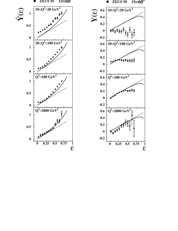
Figure 11: ZEUS results for the scaling functions $\hat{Y}(\epsilon)=-\beta\ln{(\hat{r}/\tilde{b})}/\tilde{b}$ (left) and $Y(\epsilon)=2\beta\ln{r}/\tilde{b}$ (right) for various jet energies $E=<Q>/2$; $\tilde{b}=2\beta\sqrt{\ln{(E\sin{\Theta/\Lambda})}}$. Solid lines give the scaling QCD predictions, namely $\omega(\epsilon,2)-2$, Eq. (98) and $\omega(\epsilon,2)-2\sqrt{1-\epsilon}$, Eq. (97). Dotted line shows the constant $\alpha_{s}\;$ version of the asymptotic forms, Eq. (101).

Figure 12: The same scaling functions as in Fig.11, as measured by the DELPHI Collaboration for two highest jet energies. Results of the Monte Carlo simulations are also shown.

5.3 Azimuthal Correlations to the Next-to-Leading Order

Complete next-to-leading results are available only for the azimuthal correlations among gluons emitted from a hard $q\bar{q}$ pair in an $e^{+}e^{-}$ annihilation. $\!{}^{{\bf?},{\bf?}}$ This problem is closely related to the string-drag effect and will be discussed in detail later. In short, consider emission of a soft gluon associated with the hard $q\bar{q}g$ system. Particle density is reduced around the direction opposite to the hard gluon due to the negative interference effects. In the limit when the hard gluon becomes softer interference is still destructive and one expects similar suppression.

The lowest order result for the normalized correlation reads in the soft gluon limit

$$C(\eta,\varphi)=1+{N_{C}\over 2C_{F}}{\cos{\varphi}\over\cosh{\eta}-\cos{\varphi}},$$ (102)

with $\eta$ and $\varphi$ being the rapidity and azimuthal angle differences of two soft gluons.

Theoretical improvements of this formula involve: i) corrections to the multiplicity flow, ii) corrections from the hard matrix element, and iii) resuming ${\cal O}(\alpha_{s}\ln^{2}\vartheta_{gg})$ terms similar to $\vartheta_{12}$ singularities considered in the previous section. Moreover, the sensitivity to the jet axis was eliminated by introducing a concept of the energy-multiplicity-multiplicity correlations. $\!{}^{{\bf?}}$ Additional weighting by the energy effectively defines the jet axis as the direction of a fast particle. Such a definition is simple to implement experimentally and retains all features of the QCD evolution.

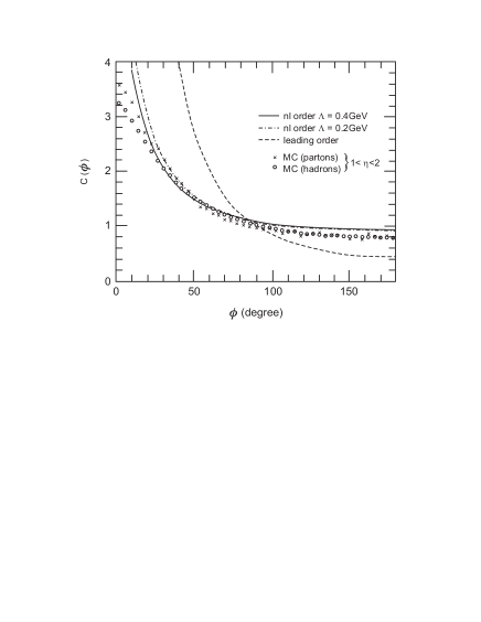
Figure 13: Azimuthal correlations of partons in a jet near central rapidity $\eta$, at leading and next-to-leading orders for different $\Lambda$ and comparison with the Monte Carlo (HERWIG) result $\!{}^{{\bf?}}$.

In Fig. 13 theoretical calculations are compared with the MC results. Indeed the back-to-back configuration ($\varphi\sim 180^{\rm o}$) is suppressed. The effect of non leading corrections is rather dramatic especially for the aligned gluons. At $\varphi=\pi$ the non leading corrections almost double the leading order result bringing theoretical predictions to within $10\%$ of the MC simulations. Measurements by OPAL and ALEPH have confirmed the above behavior. $\!{}^{{\bf?},{\bf?}}$ Experiment agrees with Monte Carlo up to $5-10\%$ in the whole range of $\varphi$ which provides satisfactory support for higher order calculations and for the LPHD. In particular, experimental numbers for the back-to-back (in the azimuth) configuration read

$$C(\pi) = 0.787\pm 0.002\pm 0.004\;\;(\rm{OPAL}),$$

$$C(\pi) = 0.783\pm 0.001\pm 0.016\;\;(\rm{ALEPH}),$$ (103)

where the first error is statistical and the second is systematic. This is to be compared with the MC result $C_{MC}=0.8$ and analytical improved $C_{NL}=0.93$.

5.4 The Critical Angle and the Local Parent Child Correspondence

The success of perturbative QCD in describing hard processes only enhances our curiosity and the need to understand soft phenomena as well. It is an experimental fact that many properties of hadronic final states are well described by equivalent partonic observables also at the scales close to, or even beyond, the standard range of applicability of perturbative QCD. This is the foundation of the Local Parton Hadron Duality hypothesis, which still inspires many theoreticians. Is it possible, that some properties of the soft, confining interactions are already hidden in the perturbative cascade? The only example of such a mechanism is provided by the pre-confinement scenario in early days of perturbative QCD. $\!{}^{{\bf?}}$ In this section we would like to discuss another intriguing property of the perturbative cascade. Namely there exist a small critical angle which is still within the range of perturbative calculations, and below which the distribution of next generation of partons is equal to the distribution of their parents. $\!{}^{{\bf?}}$ This precise coincidence of the distributions of partons from different generations, which we call the Local Parent Child Correspondence, has some interesting consequences.

Consider again the distribution of the relative angle $D^{(2)}(\vartheta_{12},P,\Theta)$ discussed earlier. In the double logarithmic approximation this correlation function obeys the integral equation which can be derived from the evolution equation (33). $\!{}^{{\bf?}}$

$$D^{(2)}(\vartheta_{12},P,\Theta)=d^{(2)}(\vartheta_{12},P,\Theta)+\int_{Q_{0}/\vartheta_{12}}^{P}\frac{dK}{K}\int_{\vartheta_{12}}^{\Theta}\frac{d\Psi}{\Psi}\gamma_{0}^{2}(K\Psi)D^{(2)}(\vartheta_{12},K,\Psi).$$ (104)

The inhomogenous term $d^{(2)}$ is constructed from the product of 1-particle angular distributions and found as $d^{(2)}(x)=D^{(1)}(x)\overline{N}(x),\;\;x=P\vartheta_{12}/\Lambda$ and with the multiplicity $\overline{N}$ in the cone of half-angle $\vartheta_{12}$ around the primary parton axis. In exponential accuracy $d^{(2)}\sim\overline{N}^{2}$.

The solution of Eq. (104) can be written as $\!{}^{{\bf?}}$

$$D^{(2)}(\vartheta_{12},\Theta,P)=\int_{Q_{0}/\vartheta_{12}}^{P}\frac{dK}{K}R\left({P\over K},{\Theta\over\vartheta_{12}},{K\vartheta_{12}\over\Lambda}\right)d^{(2)}\left({K\vartheta_{12}\over\Lambda}\right).$$ (105)

The resolvent $R\left({P\over K},{\Theta\over\vartheta_{12}},{K\vartheta_{12}\over\Lambda}\right)$ is nothing but the momentum distribution of the parent partons $K$ in the jet $(P,\Theta)$ with the condition, that their virtuality is bound from below by $K\vartheta_{12}$ and not by the elementary cut-off $Q_{0}$. This is equivalent to restricting their emission angle to be greater than $\vartheta_{12}$.

It turns out that this distribution is non analytic at some small value of the relative angle $\vartheta_{12}=\vartheta_{c}$. To see this consider the dependence of the integrand of Eq. (105) on the parent parton momentum $K$. The interplay between the decrease of the parent density $\overline{R}$ and the increase of the children densities $d^{(2)}$ with $K$ produces a sharp maximum which is however $\vartheta_{12}$ dependent. The important element of the running $\alpha_{s}\;$ analysis is that the position of this maximum is independent of $Q_{0}$, since both distributions do not depend on $Q_{0}$. Now, for small relative angles the above maximum shifts below the lower limit $Q_{0}/\vartheta_{12}$ of the momentum integration. At that point the result changes non analytically (albeit very gently — analogously to the second order phase transitions in statistical systems). Namely, for $\vartheta_{12}$ bigger than $\vartheta_{c}$, $\rho^{(2)}$ is given ( to the exponential accuracy) by the $Q_{0}$ independent value of the integrand at the maximum. For $\vartheta_{12}$ below $\vartheta_{c}$, however, the result is given by the value of the integrand at the lower bound and obviously depends on $Q_{0}$. Moreover, since $d_{2}(1)=1$ in our exponential approximation, the density of pairs below $\vartheta_{c}$ is given entirely by the density of parent partons at the minimal momentum $K=Q_{0}/\vartheta_{12}$

$$\rho^{(2)}(\vartheta_{12})\sim R\left({P\vartheta_{12}\over Q_{0}},{\Theta\over\vartheta_{12}},{Q_{0}\over\Lambda}\right).$$ (106)

The value of the critical angle derived from these considerations reads $\!{}^{{\bf?}}$

$$\vartheta_{c}={Q_{0}\over P}\left(P\Theta\over Q_{0}\right)^{1/5},\;\;\vartheta_{c}={Q_{0}\over P}\left({\ln{(P\Theta/\Lambda)}\over\ln{(Q_{0}/\Lambda)}}\right)^{4/9},$$ (107)

for the constant and running $\alpha_{s}\;$ respectively. The transverse momentum associated with this angle grows weakly with the jet momentum $P$ hence the perturbative description applies also in the new region $Q_{0}/P<\vartheta_{12}<\vartheta_{c}$. Even though some features of this result (e.g. the emergence of a sharp singularity) would be modified in more refined approximations, the existence of the two angular regions with different properties is genuine. In the large angle region, the distribution scales in $\epsilon$ (see previous section) and is independent of $Q_{0}$. On the other hand, below $\vartheta_{c}$ the distribution depends on $Q_{0}$, which can be interpreted as the sensitivity to the soft interactions where the hadronization and confinement start becoming important.

The numerical value of the critical angle is rather small at high energies, $\vartheta_{c}\mathrel{\mathop{\kern 0.0pt\hbox to0.0pt{\raise 0.86108pt\hbox{$<$}\hss}}\lower 3.87495pt\hbox{\kern-1.90002pt$\sim$}}1^{\rm o}$ at LEP energies. It is interesting to note that the scaling in $\epsilon$ is indeed best satisfied at large angles ($\vartheta_{12}\gg\vartheta_{c}$), see Fig. 12, which is consistent with this analysis.

Sensitivity to the cut-off $Q_{0}$ at small angles leads to an interesting prediction for the particle mass dependence of the produced pair. Assuming that the particle mass acts as an effective transverse momentum cutoff, we expect that the spectrum of pairs with large relative angles is mass independent, while for angles smaller than $\vartheta_{c}$ the density depends on the mass and is suppressed for higher masses.

6 On Inclusive Properties of Heavy Quark Jets

Until now we have discussed mainly the properties of jets in $e^{+}e^{-}$ collisions obtained by analyzing the full hadron data sample with contributions from all flavors. In the last few years intensive experimental studies have been performed with the heavy-quarks $Q(c,b)$. Experiments at LEP and SLC have produced a wealth of new interesting results on the profiles of jets initiated by heavy quarks. The accuracy of measurements started to be comparable with that in the $q\bar{q}$ events. This is mainly related to the steady improvement in the heavy-quark tagging efficiencies. Further progress is expected from the measurements at hadronic colliders and a future linear $e^{+}e^{-}$ collider. The principal physics issues of these studies are related not only to testing the fundamental aspects of QCD, but also to their large potential importance for measurements of heavy-particle properties: lifetimes, spatial oscillations of flavor, searching for CP-violating effects in their decays etc.

A good understanding of $b$-initiated jets is of primary interest for analysis of the final-state structure in $t\bar{t}$ production processes. A detailed knowledge of the $b$-jet profile is also essential for the Higgs search strategy.

The physics of heavy-quarks has been traditionally considered as one of the best testing grounds for QCD. Note that since the mass of $b$-quark is much larger than the QCD scale $\Lambda$, the $b$-quark fragmentation proves to be an especially useful tool for studying the perturbative scenario. In this section we will restrict ourselves to the discussion of some specific features of heavy-quark-initiated events which are related to our previous considerations of multiparticle production and LPHD.

6.1 QCD Bremsstrahlung Accompanying Heavy Quark Production

When examining the perturbatively based structure of the heavy-quark jets, one has to understand first how the development of the parton cascades generated by $Q$ depends on the quark mass $M$. It was demonstrated $\!{}^{{\bf?},{\bf?},{\bf?},{\bf?}}$ that the difference in many properties of hadronic jets initiated by heavy quarks (excluding the products of the weak decay of the heavy quark iteself), from that of light quarks, originates from the restriction of the phase space available to gluon radiation associated with the kinematic effects of the heavy-quark mass.

As well known, the radiation pattern of the primary soft gluon with energy $\omega$ from a massive relativistic quark with energy $E_{Q}\gg M$ and small emission angle $\Theta\ll 1$ is given by

$$d\sigma_{Q\rightarrow Q+g}\;=\;\frac{\alpha_{S}}{\pi}\>C_{F}\frac{\Theta^{2}d\Theta^{2}}{(\Theta^{2}+\Theta_{0}^{2})^{2}}\>\frac{d\omega}{\omega},$$ (108)

where

$$\Theta_{0}\;=\;\frac{M}{E_{Q}}.$$ (109)

From Eq. (108) one concludes that the large double-logarithmic contribution comes only from the region of relatively large radiation angles

$$\Theta\;\gg\;\Theta_{0},$$ (110)

where emission becomes insensitive to $M$ and appears to be identical to that for the light $q$-jet

$$d\sigma_{Q\rightarrow Q+g}\;=\;\frac{\alpha_{S}}{\pi}\>C_{F}\>\frac{d\Theta^{2}}{\Theta^{2}}\>\frac{d\omega}{\omega}.$$ (111)

For the region

$$\Theta\;<\;\Theta_{0}$$ (112)

the angular integration is no longer logarithmic.

As it follows from (108) the forward gluon radiation is suppressed. $\!{}^{{\bf?},{\bf?}}$ This phenomenon is characteristic for bremsstrahlung off a massive particle. It reflects the conservation of the projection of the total angular momentum on the massive fermion momentum: the soft radiation does not change the quark helicity and the forward emission is forbidden (in analogy to the well-known “$0-0$ transition” phenomenon). As it is discussed below, after taking into account parton cascades generated by a primary gluon, the relative yield of final particles due to this part of phase space is ${\cal O}(\sqrt{\alpha_{S}})$. Since the main logarithmic contribution is absent and the differential cross section (108) vanishes in the forward direction, it is natural $\!{}^{{\bf?}}$ to call this region the “dead cone”  — a relatively depopulated cone around the quark direction with an opening angle $\Theta\sim\Theta_{0}$.

Notice that the standard expression for the soft bremsstrahlung spectrum

$$d\sigma_{Q\rightarrow Q+g}\;=\;\frac{2C_{F}\alpha_{S}}{\pi}\>\frac{v^{2}\sin^{2}\Theta}{(1-v^{2}\cos^{2}\Theta)^{2}}\>\frac{d\omega}{\omega}\>d\cos\Theta$$ (113)

with

$$v\;=\;\sqrt{1-\frac{M^{2}}{E_{Q}^{2}}}$$ (114)

describes adequately the non-logarithmic region of finite emission angles $\Theta\sim 1$. This part of the radiation phase space contributes as ${\cal O}(\sqrt{\alpha_{S}})$ too. Corresponding corrections will be taken into full account later when we derive formulae for particle multiplicities outside the scope of the double logarithmic approximation.

Recall that the angular pattern in (113) is exactly the same as in the QED case of classical photon bremsstrahlung off the massive electric charge. $\!{}^{{\bf?}}$

As we mentioned above, the structure of the primary gluon radiation at large angles (110) appears to be identical to that for the light $q$-jet. The same holds true for the internal structure of secondary gluon subjects (angular-ordered cascades).

6.2 Specific Features of Events Containing Heavy Quarks

As was discussed in detail in the previous sections, the dominant role of the perturbative dynamics has been very successfully tested in studies of light-hadron distributions in QCD jets. Within the LPHD approach the quark mass-induced restriction on the gluon radiation leads to a number of important consequences for the $Q$-quark jets.

• Explicit visualization of the dead cone

From the measurements of the “companion” particle distributions inside fixed cones around the $Q$ direction one can learn about the expected depletion of the forward-particle production for angles $\Theta<\frac{M}{E_{Q}}$. Note that a study of the forward hadroproduction in $Q$-jets which is free from “trivial” perturbative bremsstrahlung effects, may help in the investigation of the subtle features of some non-trivial confinement scenarios.

The first comparison of the primary particle angular distribution in the $b$ and light-quark jets in $e^{+}e^{-}$ annihilation has been reported by DELPHI. $\!{}^{{\bf?}}$ In the data analysis special care has been taken in order to exclude the decay products of the $b$-hadrons from consideration. Preliminary results look quite encouraging. However further detailed studies are needed for establishing the perturbative-QCD origin of the observed depopulation of the forward-particle production in the $b$-quark initiated jets.

• Leading particle effect in heavy-quark fragmentation

Suppression of small angles restricts emission of hard gluons with relatively small transverse momenta $k_{\perp}$, where radiation is normally most intensive as being proportional to $\alpha_{S}(k_{\perp}^{2})$. This results in a decrease in the energy fraction that the heavy-quark $Q$ is sharing with the secondary bremsstrahlung particles. $\!{}^{{\bf?},{\bf?},{\bf?}}$ Thus, the inclusive distribution of $Q$ is expected to peak near $x_{Q}\approx 1$, the so-called leading particle effect, which first was predicted within the framework of the parton model $\!{}^{{\bf?}}$ and quantified as the so-called Peterson fragmentation. $\!{}^{{\bf?}}$ Recall that at the hadronization stage the heavy-quark loses only a momentum fraction of order $\Lambda/M$ when forming a heavy-light hadron. $\!{}^{{\bf?}}$ The leading heavy particle phenomenon has been clearly observed experimentally in the $b\bar{b}$ and $c\bar{c}$ events in $e^{+}e^{-}$ annihilation. $\!{}^{{\bf?},{\bf?}}$ As expected, at the $Z^{0}$ the $b$-quark inclusive spectra peak very close to one, around $x_{Q}\simeq 0.8-0.9$.

The record accuracy in determination of the $b$-quark spectrum has been achieved in the recent SLD measurement. $\!{}^{{\bf?}}$ As a result, this allows to discriminate between current parton-shower plus hadronization models.

As discussed in detail, $\!{}^{{\bf?}}$ within the LPHD scenario the effects of perturbative gluon radiation allow to reproduce the shape of the heavy-quark inclusive spectrum provided the perturbative prediction is extrapolated smoothly down to the region of small gluon transverse momenta within the universal low-scale $\alpha_{S}$ approach. As well known such approach proves to be quite successful in the description of the jet event shape, for a discussion, see for example, Ref. 13 and the article by V. Braun and M. Beneke in this book.

The Sudakov form-factor suppression of the quasi-elastic region at $x_{Q}\rightarrow 1$ results in the distribution which is qualitatively similar to the parton-model-motivated Peterson fragmentation function. $\!{}^{{\bf?}}$ Note that all-order resummation of the collinear and Sudakov logs have been considered also. $\!{}^{{\bf?}}$ It is worthwhile to mention, that as far as the heavy-quark is concerned, based on LPHD one may expect that a purely perturbative treatment is dual to the sum over all possible hadronic excitations. Therefore, without involving any phenomenological fragmentation function at the hadronization stage, one could attempt to describe the energy fraction distribution averaged over heavy-flavored hadron states, the mixture that often appears experimentally. Such purely perturbative approach is at least free from the problem of “double counting” which one may face when trying to combine the effects of perturbative and hadronization stages.

• Average multiplicity of events containing heavy quarks

As we discussed above, a forward suppression of soft-gluon radiation off an energetic massive quark $Q$ induces essential differences in the structure of the accompanying radiation in light- and heavy-quark-initiated jets. According to the LPHD concept, this, in particular, should lead to corresponding difference in companion multiplicity of radiated light hadrons. $\!{}^{{\bf?},{\bf?},{\bf?}}$

It is a direct consequence of the perturbative approach that the difference of companion average multiplicities of hadrons, $\Delta N_{Qq}$ from equal energy (hardness) heavy- and light-quark jets should be energy-independent (up to power correction terms ${\cal O}(M^{2}/W^{2})$. This constant is different for $c$ and $b$ quarks and depends on the type of light hadron under study (e.g. all charged, $\pi^{0}$, etc.). This is in marked contrast with the prediction of the models based on the idea of reduction of the energy scale, $\!{}^{{\bf?}}$ $N_{Q\bar{Q}}(W)=N_{q\bar{q}}((1-\langle x_{Q}\rangle)W)$, so that the difference of $q$- and $Q$-induced multiplicities grows with $W$ proportional to $N(W)$. We shall elucidate this bright prediction of the perturbative scenario .

Recall, that companion multiplicity is an infrared-sensitive quantity dominated by the emission of relatively soft gluons. In this domain the only difference between heavy- and massless-quark cases comes from the suppression of soft bremsstrahlung in the forward direction $\Theta_{1+}\lower 3.01385pt\hbox{$\;\stackrel{{\scriptstyle\textstyle<}}{{\sim}}\;$}\Theta_{0}\equiv M/E_{Q}$, where $\Theta_{1+}$ is the angle between a primary gluon $(g_{1})$ and the quark $(+)$. In the region of large gluon radiation angles $\Theta_{1+}\gg\Theta_{0}$, the finite-mass effects are power-suppressed and do not affect the picture of strictly angular-ordered evolution of $g_{1}$ as a secondary jet. It is straightforward to verify that within the MLLA accuracy the finite mass induces only a small integral correction to the angular-ordered prescription for the next-generation gluon $g_{2}$. As a result, in the large-angle region the internal structure of secondary-gluon jets is identical to that for the light-$q$ case, and the emission angle $\Theta_{1+}$ should be taken as an evolution parameter to restrict the subsequent cascading. As usual, the smaller the radiation angle $\Theta_{1+}$, the less populated with offspring partons the gluon subjet $g_{1}$ is.

The situation changes, however, when $\Theta_{1+}$ becomes smaller than $\Theta_{0}$. The dead cone region gives a sizeable (though nonleading) contribution, of order $\sqrt{\alpha_{S}}$, and should be taken into account within the MLLA. Here the opening angle of the jet $g_{1}$ “freezes” at the value $\Theta_{0}$ and no longer decreases with $\Theta_{1+}\rightarrow 0$. The reason for this is rather simple. Normally, in the “disordered” angular kinematics $\Theta_{21}\geq\Theta_{1+}$ the destructive interference between emission of a soft gluon $g_{2}$ by quark and $g_{1}$ cancels the independent radiation $g_{1}\rightarrow g_{2}$.

Meantime, in the massive-quark case the interference contribution enters the game only when $\Theta_{2+}>\Theta_{0}$, so that the cancellation of the independent $1\rightarrow 2$ term inside the $\Theta_{0}$-cone does not occur. In physical terms what happens is the loss of coherence between $+$ and $1$ as emitters of the soft gluon 2 due to accumulated longitudinal separation $\Delta z_{1+}>\lambda_{||}^{(2)}\approx\omega_{2}^{-1}$ between massless and massive charges $(v_{1}=1,v_{+}\approx 1-\Theta_{0}^{2}/2<1)$. Indeed, during the formation time of $g_{2},t_{f}^{(2)}\sim 1/\omega_{2}\Theta_{21}^{2}$ the quark and the gluon 1 separate in the longitudinal direction by

$$\Delta z_{1+}\sim t_{f}^{(2)}\>|v_{+}-\cos\Theta_{1+}|\>\sim\>\lambda_{||}^{(2)}\cdot(\Theta_{1+}^{2}+\Theta_{0}^{2})\biggr{/}\Theta_{21}^{2}.$$ (115)

It is the last factor which determines whether interference is essential or not. When this ratio is larger than unity, $Q$ and $g_{1}$ are separated enough for $g_{2}$ to be able to resolve them as two individual classical charges. In these circumstances gluon $g_{1}$ acts as an independent source of the next-generation bremsstrahlung quanta. Otherwise, no additional particles triggered by $g_{1}$ emerge on top of the yield determined by the quark charge (which equals total color charge of the $Qg_{1}$ system). In the massless limit $(\Theta_{0}=0)$ this reproduces the standard angular-ordered picture, $\Theta_{21}<\Theta_{1+}$. In the massive case one concludes from (115) that the upper limit of the relative gluon angle remains finite when $\Theta_{1+}$ falls inside the dead cone: $\Theta_{21}<\Theta_{0}$ for arbitrarily small $\Theta_{1+}\ll\Theta_{0}$.

Thus, the proper evolution parameter for subsequent parton cascading of the primary gluon $g_{1}$ (generalization of an “opening angle” of jet 1) may be chosen as

$$\tilde{\Theta}_{1+}^{2}\;\equiv\;\Theta_{1+}^{2}\>+\>\Theta_{0}^{2}.$$ (116)

Another comment is in order concerning generalization of the argument of the running coupling to the massive-quark case. Here again the substitution similar to (116) is applicable. Namely, for the effective coupling that determines the probability of the emission $Q\rightarrow Q+g_{1}$ one has to use as an argument $\!{}^{{\bf?}}$

$$k_{\perp}^{2}\;=\;\omega_{1}^{2}\left[\left(2\sin\frac{\Theta_{1+}}{2}\right)^{2}\>+\>\Theta_{0}^{2}\right]\;\approx\;\omega_{1}^{2}\>\tilde{\Theta}_{1+}^{2}.$$ (117)

Within MLLA the expression for the multiplicity of light particles accompanying the production of a heavy-quark pair, $N_{Q\bar{Q}}$, can be obtained by convoluting the probability $dw$ of a single gluon bremsstrahlung off a heavy-quark $Q$ with the parton multiplicity initiated by the gluon subjet with the hardness parameter $k_{\perp}$.

The differential first-order cross section for $e^{+}e^{-}\rightarrow Q\bar{Q}g$ integrated over the angles of the $Q\bar{Q}g$ system was first presented by Ioffe $\!{}^{{\bf?}}$ (QED first-order results can be found elsewhere $\!{}^{{\bf?}}$). For the case of vector $Q\bar{Q}$-production current the differential over the gluon energy fraction $z$

$$z\;=\;\frac{\omega_{1}}{E},\quad\quad 2E\;=\;W\;\equiv\;\sqrt{s}$$ (118)

gluon emission probability can be written as $\!{}^{{\bf?},{\bf?}}$

$$dw_{V}\;=\;\frac{C_{F}\alpha_{S}}{\pi v}\>\frac{dz}{z}\>\frac{d\eta}{\sqrt{1-\eta}}\left\{2(1-z)\>\frac{\eta-\eta_{0}}{\eta^{2}}\>+\>z^{2}\left[\frac{1}{\eta}\>-\>\frac{1}{2}\right]\>\zeta_{V}^{-1}\right\}.$$ (119)

Here

$$1\>\geq\>\eta = 1-\beta^{2}\cos^{2}\Theta_{C}\>\geq\>\eta_{0}\>=\>\frac{4m^{2}}{1-z};\quad\quad m\;\equiv\;M/W\;\ll\;1,$$

$$\zeta_{V} = (3-v^{2})/2\;=\;1\>+\>2m^{2}$$ (120)

with $\beta$ the quark velocity and $\Theta_{C}$ the polar gluon angle in the $Q\bar{Q}$ rest frame,

$$\beta^{2}\;=\;\beta^{2}(z)\;=\;1\>-\>\frac{4m^{2}}{1-z}\;\leq\;v^{2}\;=\;1\>-\>4m^{2}\;\geq\;z.$$ (121)

The first term in curly brackets contains the main (double logarithmic) contribution and corresponds to the universal soft gluon bremsstrahlung. As it follows from the celebrated Low soft bremsstrahlung theorem, $\!{}^{{\bf?}}$ extended to the fermion case by Burnett and Kroll, $\!{}^{{\bf?}}$ both $z^{-1}$ and $z^{0}$ parts of the radiation density have classical origin and are therefore process (and quark spin) independent. $\!{}^{{\bf?}}$ This first term explicitly exhibits the dead cone behaviour: forward “soft” radiation vanishes, $\eta\rightarrow\eta_{0}$ when $\sin\Theta_{C}\rightarrow 0$. The second term which is proportional to $z^{1}$ (hard gluons) depends, in principle, on the $Q\bar{Q}$ production mechanism. Namely, both $-\frac{1}{2}$ subtraction term and the $\zeta$-factor may be different for the different production currents. $\!{}^{{\bf?},{\bf?}}$ This indicates that already at the level of $\alpha_{S}$ corrections the average companion multiplicity acquires a process-dependent contribution from the three-jet ensembles and, thus, cannot be treated any more as an intrinsic characteristic of the $Q\bar{Q}$ system.

Neglecting now the corrections of relative order $\alpha_{S}$ and $m^{2}$ the average companion multiplicity $N_{Q\bar{Q}}(W)$ can be given by

$$N_{Q\bar{Q}}(W) = \frac{C_{F}}{\pi}\>\int_{0}^{v^{2}}\>\frac{dz}{z}\>\int_{\eta_{0}}^{1}\left\{\frac{d\eta}{\eta}\>\frac{1+(1-z)^{2}}{\sqrt{1-\eta}}\right.$$ (122)

$$-\;\left.\frac{\eta_{0}d\eta}{\eta^{2}}\>2(1-z)\right\}\>\left(\alpha_{S}(k_{\perp})\>N_{G}(k_{\perp})\right)$$

with $k_{\perp}^{2}=(zW/2)^{2}\eta$. Note that the second term in the curly brackets is non-logarithmic in $\eta$ and generates next-to-leading correction $\delta_{1}N\sim\sqrt{\alpha_{S}(M)}N(M)$, see below.

The main contribution to $N_{Q\bar{Q}}$ comes from the DL phase-space region. Meanwhile, the expression (122) keeps track of significant SL effects as well, provided that the multiplicity factor $N_{G}$ is calculated with the MLLA accuracy.

Introducing a convenient variable

$$\kappa^{2}\;=\;\frac{E^{2}}{\omega_{1}^{2}}\>k_{\perp}^{2}\;=\;E^{2}\left[\left(2\sin\>\frac{\Theta_{1+}}{2}\right)^{2}\>+\>\Theta_{0}^{2}\right],$$ (123)

one can rewrite Eq. (122) as

$$N_{Q\bar{Q}}(W)\;=\;2\int_{M^{2}}^{W^{2}}\frac{d\kappa^{2}}{\kappa^{2}}\left[1-\frac{M^{2}}{\kappa^{2}}\right]\>\int_{Q_{0}}^{\kappa}\;\frac{dk_{\perp}}{\kappa}\;\>P_{q}^{g}(z)\;\frac{\alpha_{S}(k_{\perp})}{2\pi}\>N_{G}(k_{\perp}),$$ (124)

with $k_{\perp}=z\kappa$. Here $P_{q}^{g}$ stands for the standard DGLAP kernel and $Q_{0}$ denotes a transverse momentum cut-off as used in the previous sections. In the massless limit $M\lower 3.01385pt\hbox{$\;\stackrel{{\scriptstyle\textstyle<}}{{\sim}}\;$}Q_{0}$ the contribution of the $M^{2}/\kappa^{2}$ term vanishes and (124) reproduces the known result for the $q$-jet multiplicity. The integration can be performed with the use of the relation corresponding to the evolution equation for light-quark jet multiplicity:

$$N_{q}^{\prime}(Q)\;\equiv\;\frac{\partial}{\partial\ln Q^{2}}\>N_{q}(Q/2)\;=\;\int_{Q_{0}}^{Q}\>\frac{dk_{\perp}}{Q}\>P_{q}^{g}(z)\>\frac{\alpha_{S}(k_{\perp})}{2\pi}\;N_{G}(k_{\perp}),$$ (125)

with

$$N_{q\bar{q}}(Q)\;=\;2N_{Q}\>\left(\frac{Q}{2}\right),$$ (126)

see Section 3. Then Eq. (124) takes the form

$$N_{Q\bar{Q}}(W)\;=\;N_{q\bar{q}}(W)\>-\>2N_{q}\left(\frac{M}{2}\right)\>-\>2N_{q}^{\prime}\left(\frac{M}{2}\right)\>+\>{\cal O}(\alpha_{S}N_{q};\Theta_{0}^{2}N_{q}^{\prime}).$$ (127)

Notice that the factor 2 in the argument of $N_{q}$ generates $\sqrt{\alpha_{S}}N_{q}(M)$ correction and is under control in the present analysis whereas it could be omitted in the $N_{q}^{\prime}$ terms as producing $\alpha_{S}N_{q}(M)$ terms which we neglected systematically in (124). Within this accuracy the term $N^{\prime}\sim\sqrt{\alpha_{S}}N_{q}(M)$ can be embodied into the multiplicity factor by shifting its argument, namely

$$N_{q}\left(\frac{M}{2}\right)\>+\>N_{q}^{\prime}\left(\frac{M}{2}\right)\>\approx\>N_{q}\left(M\frac{\sqrt{e}}{2}\right).$$ (128)

Finally we arrive at the formula expressing the companion multiplicity in $e^{+}e^{-}\rightarrow Q\bar{Q}$ in terms of that of $e^{+}e^{-}\rightarrow q\bar{q}$ (assuming $M\gg\Lambda$)

$$N_{Q\bar{Q}}(W)\;=\;N_{q\bar{q}}(W)\>-\>N_{q\bar{q}}(\sqrt{e}M)\>[1+{\cal O}(\alpha_{S}(M))].$$ (129)

The total particle multiplicity in $Q\bar{Q}$ events then reads as

$$N^{e^{+}e^{-}\rightarrow Q\bar{Q}}(W)\;=\;N_{Q\bar{Q}}(W)\>+\>n_{Q}^{dk},$$ (130)

where $n_{Q}^{dk}$ stands for the constant decay multiplicity of the heavy-quarks $(n_{Q}^{dk}=11.0\pm 0.2$ for $b$-quarks, $n_{Q}^{dk}=5.2\pm 0.3$ for $c$-quarks $\!{}^{{\bf?}}$).

Some comments are in order here. The main consequence of (130) is that the difference between particle yields from $q$- and $Q$-jets at fixed energy $W$ depends on the heavy-quark mass and remains $W$-independent. $\!{}^{{\bf?},{\bf?},{\bf?}}$ The question arises, to what extent this difference can be quantitatively predicted? An important issue concerns non-leading corrections $\sim{\cal O}(\alpha_{S}(W))$ to the main term. From the first sight one may expect that instead of (129) the correct formula would look like

$$N_{Q\bar{Q}}(W) = \{N_{q\bar{q}}(W)\}^{\rm MLLA}\>[1+{\cal O}(\alpha_{S}(W))]$$ (131)

$$\quad\quad\quad-\>\{N_{q\bar{q}}(\sqrt{e}M)\}^{\rm MLLA}\>[1+{\cal O}(\alpha_{S}(M))],$$

where $\{N\}^{\rm MLLA}$ denotes the MLLA multiplicities accounting for the $\sqrt{\alpha_{S}}+\alpha_{S}$ effects in the anomalous dimension and $1+\sqrt{\alpha_{S}}$ terms in the normalization (coefficient function). Meantime, because of the steep growth of the multiplicity (faster than any power of $\ln W$) the neglected, order $\sqrt{\alpha_{S}(W)}N(W)$ terms would dominate over the finite subtraction term in (131) with increasing energy. Thus, the very possibility to discriminate between the $Q$- and $q$-quark jets within the present theoretical accuracy may be endangered. However, a close inspection of the subleading corrections to Eq. (129) (proportional to $N_{q\bar{q}}(W)$) shows that all of them are independent of the heavy-quark mass $M$. Thus, the first corrections of order $\alpha_{S}(W)N_{q\bar{q}}(W)$ arise either from further improvement of the description of anomalous dimension $\Delta\gamma(\alpha_{S})\sim\alpha_{S}^{2}$ determining intra-jet cascades, or from ${\cal O}(\alpha_{S}(W))$ terms in the coefficient function due to

• 3-jet configuration quark + antiquark + hard gluon at large angles,

• the so-called “dipole correction” to the angular-ordering scheme quark + antiquark + two soft gluons with large emission angles, $\!{}^{{\bf?}}$

which are insensitive to the $\Theta_{0}$ value with the power accuracy $\sim\Theta_{0}^{2}\ll 1$. Therefore, replacing the approximate MLLA multiplicity factors in (131) by the real observable multiplicities, one arrives at (129) which makes it possible to establish a phenomenological relation between light and heavy-quark jets with relative accuracy $\sqrt{\alpha_{S}(M)}\>M^{2}/W^{2}$.

Thus, the difference between particle yields from $q$- and $Q$-jets at fixed annihilation energy $W$ proves to be $W$-independent  $\!{}^{{\bf?},{\bf?},{\bf?}}$

$$\delta_{Qq} = N^{e^{+}e^{-}\rightarrow Q\bar{Q}}(W)\>-\>N^{e^{+}e^{-}\rightarrow q\bar{q}}(W)\;=\;{\rm const}\>(W),$$

$$\delta_{bc} = N^{e^{+}e^{-}\rightarrow b\bar{b}}(W)\>-\>N^{e^{+}e^{-}\rightarrow c\bar{c}}(W)\;=\;{\rm const}\>(W).$$ (132)

Let us emphasize that it is the QCD coherence which plays a fundamental role in the derivation of this result. Due to this the gluon bremsstrahlung off massive and massless quarks differ only at parametrically small angles $\Theta\lower 3.01385pt\hbox{$\;\stackrel{{\scriptstyle\textstyle<}}{{\sim}}\;$}\Theta_{0}\equiv M/E$ where, due to the angular-ordering, cascading effects are majorated by the $N^{\prime}(M)$ factor.

The results of experiments on multiplicities in $b\bar{b}$ and $c\bar{c}$ events of $e^{+}e^{-}$ annihilation $\!{}^{{\bf?},{\bf?}}$ show that to the available accuracy the differences $\delta_{bq}$ and $\delta_{cq}$ are fairly independent of $W$. This is in marked contrast to the steeply rising total multiplicity and confirms the MLLA expectations. As illustrated in Fig. 14 the data on $\delta_{bq}$ are clearly inconsistent with a model $\!{}^{{\bf?}}$ based on the reduction of the energy scale. $\!{}^{{\bf?}}$

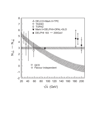
Figure 14: The difference $\delta_{bq}^{ch}$ between the average charged multiplicities of $b$- and light-quark events. $\!{}^{{\bf?}}$ The perturbative expectation is chosen as the average of the experimental values of $\delta_{bq}^{ch}$ up to the $Z^{0}$. Also shown is the prediction of the model based on the reduction of the energy scale (independently of the quark flavor).

We turn now to the absolute values of the charged multiplicity difference $\delta_{cq}^{ch}$. Neglecting in Eq. (129) the subleading ${\cal O}(\alpha_{S})$ corrections, the following MLLA expectation was found $\!{}^{{\bf?}}$ by inserting the appropriate experimental numbers into the r.h.s. of Eqs. (129)–(130):

$$\delta_{bq}^{ch}\;=\;5.5\>\pm\>0.8.$$ (133)

This exceeds the experimental values in Fig. 14, showing the essential role of the next-to-MLLA (order $\alpha_{S}(M)\cdot N(M)$) terms. An attempt was made $\!{}^{{\bf?}}$ to improve Eq. (129). However, we have to mention here that the very picture of accompanying multiplicity being induced by a single cascading gluon $\!{}^{{\bf?}}$ is not applicable at the level of subleading effects. Therefore, a self-consistent reliable theoretical improvement of the MLLA predictions for the absolute values of $N_{Qq}$ remains to be achieved.

Further detailed experimental results could provide stringent tests of the perturbative predictions. It will be very interesting to check whether the differences $\delta_{bq}^{h}$ of mean multiplicities for the identified particles remain energy independent. Results from the $Z^{0}$ are available as reference values. In particular, the DELPHI data $\!{}^{{\bf?}}$ suggest $\delta_{bq}^{\pi^{0}}\simeq 0$ and therefore, using again Eqs. (129)–(130), one may expect the relation

$$N_{\pi^{0}}^{e^{+}e^{-}\rightarrow b\bar{b}}/N_{\pi^{0}}^{e^{+}e^{-}\rightarrow q\bar{q}}\;\simeq\;1.$$ (134)

The energy behaviour of $\delta_{Qq}^{h}$ should be watched closely at a future linear collider.

• Spectra of light particles from the heavy-quark jets

The bremsstrahlung-suppression effect on the energy spectra of light particles accompanying $Q\bar{Q}$ production can be examined in a very similar way to the average multiplicity considered above. The resulting companion particle distribution $D_{Q}^{h}(x,\ln(E/\Lambda))$ is predicted to be depopulated in the hard momentum region compared with the case of the light-quark $D_{q}^{h}(x,\ln E/\Lambda)$. $\!{}^{{\bf?},{\bf?}}$ It is instructive to first gain insight by considering the double-logarithmic result. Due to the dead-cone phenomenon the difference between $D_{Q}^{h}$ and $D_{q}^{h}$ is connected with the gluon radiation at angles $\Theta<\Theta_{0}$. Radiation in the restricted angular cone is similar to the $q$-jet production process with the characteristic hardness $M\gg\Lambda$. This process induces a gluon radiation pattern with the corresponding cascading which leads to a certain final system of light hadrons. Now, boosting this jet with the Lorentz-factor $\gamma=E/M$ along the direction of its momentum one arrives at an exact image of the dead cone: an ensemble of energetic particles (with energies up to $E$) concentrated inside the cone $\Theta_{0}$. Thus, with the double logarithmic accuracy a simple formula for the $Q$-jet particle distribution can be written $\!{}^{{\bf?},{\bf?}}$

$$D_{Q}^{h}\left(x,\ln\>\frac{E}{\Lambda}\right)\;=\;D_{q}^{h}\left(x,\ln\>\frac{E}{\Lambda}\right)\>-\>D_{q}^{h}\left(x,\ln\>\frac{M}{\Lambda}\right).$$ (135)

Here the structure of the heavy-quark jet is expressed in terms of the particle distribution generated by the light-quark at different energy scales: $Q^{2}$ and $M^{2}$. In Eq. (135) $x$ is the light-hadron energy fraction, $x=E_{h}/E\lower 3.01385pt\hbox{$\;\stackrel{{\scriptstyle\textstyle>}}{{\sim}}\;$}\Lambda/M$. Therefore the depopulation occurs for quite energetic particles only, whereas in the soft domain

$$\Lambda\;\lower 3.01385pt\hbox{$\;\stackrel{{\scriptstyle\textstyle<}}{{\sim}}\;$}\;E_{h}\;\lower 3.01385pt\hbox{$\;\stackrel{{\scriptstyle\textstyle<}}{{\sim}}\;$}\;E\>\frac{\Lambda}{M}$$ (136)

the light-hadron spectra in the $Q$- and light-quark jets should be identical.

In order to obtain the MLLA result one has to take into account, first of all, the energy loss by heavy-quark at the first steps of the evolution. Using the evolution equations the expression for the $Q$-jet companion particle spectrum can be approximately given by

$$D_{Q}^{h}\left(x,\ln\>\frac{W}{\Lambda}\right)\;=\;D_{q}^{h}\left(x,\ln\>\frac{W}{\Lambda}\right)\>-\>D_{q}^{h}\left(\frac{x}{\langle y\rangle};\;\ln\>\frac{M\sqrt{e}}{\Lambda}\right)$$ (137)

where $D_{q}^{h}(x,\ln W/\Lambda)$ is the standard spectrum of particles in a $q$-jet and $\langle y\rangle$ being the averaged scaled energy fraction of the $Q$. This problem needs further detailed studies.

Measurements of the inclusive charged particle distributions in $b$- and $uds$-quark events at the $Z^{0}$ $\!{}^{{\bf?}}$ clearly show that for $b$-quarks the momentum spectrum is significantly softer than for $uds$ quarks. Unfortunately so far no comparison with the analytical QCD expectations has been performed.

7 Color-Related Phenomena in Multi-Jet Events

7.1 Radiophysics of Hadronic Flows

Coherence phenomenon is an intrinsic property of QCD (and in fact of any gauge theory). Its observation is important in the study of strong interactions and in the search for deviations from the Standard Model. As we have already discussed, within the LPHD scenario, an intimate connection is expected between the multi-jet event structure and the underlying color dynamics at small distances. The detailed features of the parton-shower system, such as the flow of color, governs the distribution of color-singlet hadrons in the final state (see e.g. Refs. 15,146).

Color coherence effects in hadron multiplicity flows in the inter-jet regions have been very well established from the early 1980’s in $e^{+}e^{-}$ annihilation, see Refs. 147,148,106,149,150, in what has been termed the “string” $\!{}^{{\bf?}}$ or “drag” $\!{}^{{\bf?}}$ effect. As discussed below the existing data are clearly in favour of QCD coherence, in particular, particle production in the region between the quark and antiquark jets in $e^{+}e^{-}\rightarrow q\bar{q}g$ events is suppressed. In pQCD such effects arise from interference between the soft gluons radiated from the $q,\bar{q}$ and $g$. $\!{}^{{\bf?},{\bf?}}$ The PETRA/PEP data first convincingly demonstrated that the wide-angle particles do not belong to any particular jet but have emission properties dependent on the overall jet ensemble. The inter-jet-coherence phenomena were then successfully studied at LEP, TRISTAN and TEVATRON (also discussed in recent reviews $\!{}^{{\bf?},{\bf?},{\bf?}}$). The experiments have nicely demonstrated the connection between color and hadronic flows.

Surely, it is entirely unremarkable that the quantum mechanical interference effects are observed in QCD. Of real importance is that the experiment proves that these effects survive the hadronization phase.

The inter-jet coherence deals with the angular structure of particle flow when three or more hard partons are involved. The hadron distribution proves to depend upon the geometry and color topology of the hard-parton skeleton. The clear observation of inter-jet-interference effects gives another strong evidence in favor of the LPHD concept. The collective nature of multiparticle production reveals itself here via the QCD wave properties of the particle flows.

The detailed experimental studies of the color-related effects are of particular interest for better understanding of the dynamics of hadroproduction in the multi-jet events. For instance, under special conditions some subtle interference effects, breaking the probabilistic picture, may even become dominant. $\!{}^{{\bf?},{\bf?}}$ We recall that QCD radiophysics predicts both attractive and repulsive forces between the active partons in the event. Normally the repulsion effects are small, but in the case of color-suppressed ${\cal O}(1/N_{C}^{2})$ phenomena they may play a leading role. It should be noted that usually the inter-jet drag effects are viewed only on a completely inclusive basis, when all the constituents of the multi-element color antenna are simultaneously active. $\!{}^{{\bf?},{\bf?}}$

A challenging possibility to operate within the perturbative scenario with the complete collective picture of an individual event (at least at very high energies) was first discussed in Ref. 155. The topologometry on the event-by-event basis could turn out to be more informative than the results of measurements averaged over the events. $\!{}^{{\bf?},{\bf?},{\bf?}}$ Note, that there is an essential difference between the perturbative radiophysics and the parton-shower Monte Carlo models. The latter not only allow but even require a completely exclusive probabilistic description. Normally (such as in the case of $e^{+}e^{-}\rightarrow q\bar{q}g$) the two pictures work in a quite peaceful coexistence; the difference only becomes drastic when one deals with the small color-suppressed effects.

Note that in spite of theoretical uncertainties, the phenomenological success of the Monte Carlo models which include interfering gluons indicates that the color-suppressed interference terms do not induce a very large effect.

Let us emphasize that the relative smallness of the non-classical effects by no means diminishes their importance. This consequence of QCD radiophysics is a serious warning against the traditional ideas of independently evolving partonic subsystems. So far (despite the persistent pressure from the theorists) no clear evidence has been found experimentally in favour of the non-classical color-suppressed effects in jets, and the peaceful coexistence between the perturbative inter-jet coherence and color-topology-based fragmentation models remains unbroken. However, these days the color-suppressed interference effects attract increased attention. This is partly boosted by the findings that the QCD interference (interconnection) between the $W^{+}$ and $W^{-}$ hadronic decays could affect the precise $W$ mass reconstruction at LEP-2, for example, $\!{}^{{\bf?},{\bf?}}$ QCD interconnection may affect also the top quark studies, in particular, its mass reconstruction. $\!{}^{{\bf?}}$

It is worthwhile to mention that the relative smallness of the color-suppressed interference effects is supported by recent searches by OPAL of the so-called reconnection effects in hadronic $Z^{0}$ decays. $\!{}^{{\bf?}}$ Finally, we recall that color-related collective effects could become a phenomenon of large potential value as a new tool helping to distinguish the new physics signals from the conventional QCD backgrounds. $\!{}^{{\bf?},{\bf?},{\bf?},{\bf?},{\bf?},{\bf?}}$

In the next subsections we briefly survey the basic ideas related to QCD collective effects in multi-jet events and then we describe (wherever possible) the latest data on QCD radiophysics.

7.2 String/Drag Effect in $q\bar{q}g$ Events

The first (and still best) example of the inter-jet color-related phenomena is the string/drag effect in $e^{+}e^{-}\rightarrow q\bar{q}g$. Since the new results based on the refined analysis of $q\bar{q}g$ events continue to pour out from the LEP groups it seems useful to recall the main ideas $\!{}^{{\bf?}}$ of the pQCD explanation of this bright coherence phenomenon. We consider first the angular distribution of particle flows at large angles to the jets in $e^{+}e^{-}\rightarrow q\bar{q}g$. The more general case including the inside jet particle flow will be discussed below.

Let all the angles $\Theta_{ij}$ between jets and the jet energies $E_{i}$ be large $(i=\{+-1\}\equiv\{q\bar{q}g\}):\Theta_{+-}\sim\Theta_{+1}\sim\Theta_{-1}\sim 1,E_{1}\sim E_{+}\sim E_{-}\sim E\sim W/3$. As was discussed above, within the perturbative picture the angular distribution of soft inter-jet hadrons carries information about the coherent gluon radiation off the color antenna formed by three emitters ($q,\bar{q}$ and $g$). The wide-angle distribution of a secondary soft gluon $g_{2}$ displayed in Fig. 15 can be written as

$$\frac{8\pi dN_{q\bar{q}g}}{d\Omega_{\vec{n}_{2}}}\;=\;\frac{1}{N_{C}}\>W_{\pm 1}(\vec{n}_{2})\>N_{g}^{\prime}(Y_{m})\;=\;\left[(\widehat{1+})\>+\>(\widehat{1-})\>-\>\frac{1}{N_{C}^{2}}\>(\widehat{+-})\right]\>N_{g}^{\prime}(Y_{m}).$$ (138)

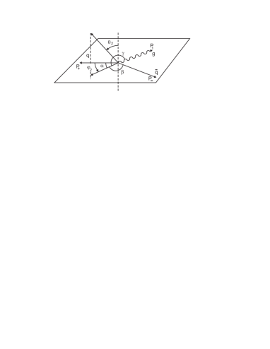
Figure 15: Kinematics of inter-jet radiation in three-jet events.

Here the “antenna” $(\widehat{ij})$ is represented as

$$(\widehat{ij})\;=\;\frac{a_{ij}}{a_{i}a_{j}},\quad\quad a_{ij}\;=\;(1-\vec{n}_{i}\vec{n}_{j}),\quad\quad a_{i}\;=\;(1-\vec{n}_{2}\vec{n}_{i})$$ (139)

and $N_{g}^{\prime}(Y_{m})$ is the so-called cascading factor taking into account that a final soft particle is a part of cascade (see Refs. 64,15 and Section 3), $N_{g}^{\prime}(Y)\equiv dN_{g}/dY$. Furthermore, $Y_{m}=\ln E\Theta_{m}/\Lambda$, where one defines the angle $\Theta_{m}={\rm min}\{\Theta_{+},\Theta_{-},\Theta_{1}\}$ with $\cos\Theta_{i}=\vec{n}_{2}\vec{n}_{i}$ for $i=\{+,-,1\}$.

The radiation pattern corresponding to the case when a photon $\gamma$ is emitted instead of a gluon reads

$$\frac{8\pi dN_{q\bar{q}\gamma}}{d\Omega_{\vec{n}_{2}}}\;=\;\frac{1}{N_{C}}\>W_{+-}(\vec{n}_{2})\>N_{g}^{\prime}(Y_{m})\;=\;\frac{2C_{F}}{N_{C}}\>(\widehat{+-})\>N_{g}^{\prime}(Y_{m}).$$ (140)

The dashed line in Fig. 16 displays the corresponding “directivity diagram”, which represents the particle density (140) projected onto the $q\bar{q}\gamma$ plane:

$$W_{+-}(\varphi_{2}) = 2C_{F}\>\int\>\frac{d\cos\Theta_{2}}{2}\>(\widehat{+-})\;=\;2C_{F}\>a_{+-}\>V(\alpha,\beta),$$

$$V(\alpha,\beta) = \frac{2}{\cos\alpha-\cos\beta}\>\left(\frac{\pi-\alpha}{\sin\alpha}\>-\>\frac{\pi-\beta}{\sin\beta}\right);\alpha\>=\>\varphi_{2},\;\beta\>=\>\Theta_{+-}-\varphi_{2}.$$

The expression $W_{+-}(\vec{n}_{2})$ is simply related to the particle distribution in two-jet events $e^{+}e^{-}\rightarrow q(p_{+})+\bar{q}(p_{-})$, Lorentz boosted from the quark cms to the lab system.

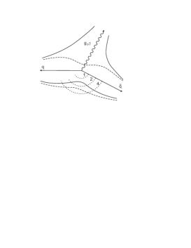
Figure 16: Directivity diagram of soft gluon radiation, projected onto the $q\bar{q}\gamma$ (dashed line) and $q\bar{q}g$ (solid) event planes. Particle flows of Eqs. (7.2) and (142) are drawn in polar coordinates: $\Theta=\varphi_{2},r=\ln 2W(\varphi_{2})$. Dotted circles show the constant levels of particle flow: $W(\varphi_{2})=1,2,4$.

Replacing $\gamma$ by $g_{1}$ changes the directivity diagram essentially because the antenna element $g_{1}$ now participates in the emission as well. However, this change leads not only to an appearance of an additional particle flow in the $g_{1}$ direction. Integrating (138) over $\Theta_{2}$ one obtains $(\gamma=\Theta_{1+}+\varphi_{2})$:

$$W_{\pm 1}(\varphi_{2})\;=\;N_{C}\>\left[a_{+1}V(\alpha,\gamma)\>+\>a_{-1}V(\beta,\gamma)\>-\>\frac{1}{N_{C}^{2}}\>a_{+-}V(\alpha,\beta)\right].$$ (142)

Fig. 16 illustrates that the particle flow in the direction opposite to $\vec{n}_{1}$ appears to be considerably lower than in the photon case. So, the destructive interference diminishes radiation in the region between the quark jets giving a surplus of radiation in the $q-g$ and $\bar{q}-g$ valleys. One easily sees that the color-coherence phenomena strongly affect the total three-dimensional shape of particle flows in three-jet events, practically excluding the very possibility of representing it as a sum of three parton contributions.

Let us recall here that, owing to coherence, the radiation of a soft gluon $g_{2}$ at angles larger than the characteristic angular size of each parton jet proves to be insensitive to the jet internal structure: $g_{2}$ is emitted by a color current which is conserved when the jet splits. This is the reason why one may replace each jet by its parent parton with $p_{i}^{2}\approx 0$.

For illustration of the particle drag phenomenon it is instructive $\!{}^{{\bf?}}$ to examine the fully symmetric $q\bar{q}g$ events (Mercedes-type topology) where $\vec{n}_{+}\vec{n}_{-}=\vec{n}_{+}\vec{n}_{1}=\vec{n}_{-}\vec{n}_{1}$. Let us take $\vec{n}_{2}$ pointing in the direction opposite to $\vec{n}_{1}$, i.e. midway between quarks. Thus, neglecting the weak dependence $N_{g}^{\prime}$ on $\Theta$, one arrives at the ratio (numbers for $N_{C}=3$)

$$\frac{dN_{q\bar{q}g}/d\vec{n}_{2}}{dN_{q\bar{q}\gamma}/d\vec{n}_{2}}\;=\;\frac{N_{C}^{2}-2}{2(N_{C}^{2}-1)}\;\approx\;0.44.$$ (143)

The corresponding ratio for the projected particle flows obtained from (7.2) and (142) reads

$$\frac{dN_{q\bar{q}g}/d\varphi_{2}}{dN_{q\bar{q}\gamma}/d\varphi_{2}}\;\approx\;\frac{9N_{C}^{2}-14}{14(N_{C}^{2}-1)}\;\approx\;0.60.$$ (144)

We emphasize that Eq. (138) provides not only the planar picture, but the global three-dimensional wide-angle pattern of particle flows.

For hadron states associated with the $\bar{q}qg$ and $\bar{q}q\gamma$ events the above ratios of particle flows should remain asymptotically correct, since non-perturbative hadronization effects are expected to cancel at high energies. It is an interesting question, to what extent the non-perturbative effects are important at present energies for a quantitative description of the data.

The analysis of the bremsstrahlung pattern clearly demonstrates particle “drag” by the gluon jet $g_{1}$. If one drops the color suppressed contribution, the two remaining terms in Eq. (138) may be interpreted as the sum of two independent $(\widehat{1+})$ and $(\widehat{1-})$ antenna patterns, boosted from their respective rest frames into the overall $q\bar{q}g$ cms. The point is, that by neglecting the $1/N_{C}^{2}$ terms, the hard gluon can be treated as a quark-antiquark pair. In this approximation each external quark line is uniquely connected to an external antiquark line of the same color, forming colorless $q\bar{q}$ antennae. In the general case, when calculating the resultant soft-radiation pattern, one can only deal with a set of such color-connected $q\bar{q}$ pairs because the interference between gluons emitted from non-color-connected lines proves to be suppressed by powers of $1/N_{C}^{2}$. $\!{}^{{\bf?},{\bf?},{\bf?},{\bf?}}$

Note that in the first order in $\alpha_{S}$ the $q\bar{q}$-antenna pattern (140) can be presented in the form $\!{}^{{\bf?}}$

$$dw_{q\bar{q}\gamma}\;=\;C_{F}\>\frac{\alpha_{S}(k_{\perp})}{\pi}\>\frac{dk_{\perp}^{2}}{k_{\perp}^{2}}\>dy_{||}$$ (145)

where

$$y_{||}\;=\;\frac{1}{2}\>\ln\frac{(p_{+}\cdot k_{2})}{(p_{-}\cdot k_{2})},\quad k_{\perp}^{2}\;=\;\frac{2(p_{+}\cdot k_{2})(p_{-}\cdot k_{2})}{(p_{+}\cdot p_{-})}$$ (146)

are the Lorentz-invariant generalizations of the rapidity and the transverse momentum of $g_{2}$ in the $q\bar{q}$ cms correspondingly. Eq. (145) describes the structure of the gluon radiation in $e^{+}e^{-}\rightarrow q\bar{q}$ events. Due to color coherence the particle multiplicity in a secondary gluon jet $g_{2}$ depends on the transverse momentum $k_{\perp}$ of the gluon and not on its energy. $\!{}^{{\bf?},{\bf?}}$ The radiation antenna formalism $\!{}^{{\bf?},{\bf?}}$ is closely related to the Lund color dipole approach. $\!{}^{{\bf?}}$ In both schemes the natural choice for the cut-off parameter in the cascades is the gluon transverse momentum in the cms of the emitting antenna-dipole. This implies that the soft gluons connect the active hard partons in exactly the same way as the string in the Lund string fragmentation model, $\!{}^{{\bf?}}$ which illustrates the connection between pQCD and the string model. $\!{}^{{\bf?}}$ Notice, however, that within the latter model there is no string piece spanned directly between the quark and antiquark, no particles are produced in between them, except by some minimum “leakage” from the other two regions.

When a gluon is emitted in, let us say, an $e^{+}e^{-}$ annihilation event, then the radiation of a second softer gluon is described by two antennas-dipoles, one spanned between the $q$ and $g$ and another between the $g$ and $\bar{q}$. The emission of a third, still softer, gluon is described in terms of three antennas-dipoles etc. The gluons appear to be color-ordered in such a way that the dipole is stretched between the color charge of one gluon and the corresponding anticolor charge of the next. Thus, neglecting the $1/N_{C}^{2}$ terms, the QCD cascade is formulated as a branching process in which antennas-dipoles are successfully split into the smaller and smaller ones.

7.3 Multiplicity Flows in Three-Jet Events

We begin here by comparing particle flows in $q\bar{q}g$ and $q\bar{q}\gamma$ events and in the next subsection we consider the respective total event multiplicities.

In what follows we first do not refer to a particular three-jet-event selection method but focus on the soft radiation by the $q\bar{q}g$ system for three given angular directions. $\!{}^{{\bf?},{\bf?}}$

In the leading order in $\alpha_{S}$ the massless parton kinematics is unambiguously fixed as follows:

$$x_{+}\;=\;2\>\frac{\sin\Theta_{1-}}{\Sigma\sin\Theta_{ij}},\quad x_{-} = 2\>\frac{\sin\Theta_{1+}}{\Sigma\sin\Theta_{ij}},\quad x_{1}\;=\;2\>\frac{\sin\Theta_{+-}}{\Sigma\sin\Theta_{ij}},$$

$$x + x_{-}\>+x_{1}\;=\;2,$$

with $x_{i}=2E_{i}/W$ being the normalized parton energies and $\Theta_{ij}$ the angles between partons $i$ and $j(+,-\equiv q,\bar{q};1\equiv g_{1})$. We emphasize here, that, owing to color-coherence, the radiation of a secondary gluon $g_{2}(k_{2}\ll E_{i})$ at angles larger than the aperture of each parton jet is insensitive to the jet internal structure.

Let us turn to the radiation pattern for $q\bar{q}\gamma$ events. In the previous subsection we considered the radiation at large angles to the jet directions, here we include the small-angle radiation in MLLA. The angular distribution of particle flow can be written as

$$\frac{8\pi dN_{q\bar{q}\gamma}}{d\Omega_{\vec{n}_{2}}}\;=\;\frac{2}{a_{+}}\>N_{g}^{\prime}(Y_{q+},Y_{q})\>+\>\frac{2}{a_{-}}\>N_{q}^{\prime}(Y_{\bar{q}-},Y_{\bar{q}})\>+\>2I_{+-}\>N_{q}^{\prime}(Y),$$ (148)

where

$$Y_{q(\bar{q})}\;=\;\ln\frac{E_{q(\bar{q})}}{\Lambda},\;Y_{q+}\>=\>\ln\left(\frac{E_{q}\sqrt{a_{+}/2}}{\Lambda}\right),\;Y_{\bar{q}_{-}}\>=\>\ln\left(\frac{E_{q}\sqrt{a_{-}/2}}{\Lambda}\right),\;Y\>\equiv\>\ln\frac{E}{\Lambda}$$ (149)

and

$$I_{+-}\;=\;(\widehat{+-})\>-\>\frac{1}{a_{-}}\>-\>\frac{1}{a_{+}}\;=\;\frac{a_{+-}-a_{+}-a_{-}}{a_{+}a_{-}}.$$ (150)

The factor $N_{A}^{\prime}(Y_{i},Y)\equiv(d/dY_{i})N_{A}(Y_{i},Y)$ takes into account that the final registered hadron is a part of cascade. $N_{A}(Y_{i},Y)$ stands for the multiplicity in a jet $A(A=q,g)$ with the hardness scale $Y$ of particles concentrated in the cone with an angular aperture $\Theta_{i}$ around the jet direction $\vec{n}_{i}$. To understand the meaning of the quantity $N_{A}(Y_{i},Y)$ it is helpful to represent it as

$$N_{A}(Y_{i},Y) = \sum_{B=q,g}\>\int_{0}^{1}\>dz\>z\>\overline{D}_{A}^{B}(z,\Delta\xi)\>N_{B}(\overline{Y}_{i}),$$

$$\Delta\xi = \frac{1}{b}\>\ln(Y/\overline{Y}_{i}),\quad\overline{Y}_{i}\;=\;Y_{i}\>+\>\ln\>z\;=\;\ln\left(\frac{zE}{\Lambda}\>\sqrt{\frac{a_{i}}{2}}\right).$$ (151)

Here $N_{B}(\overline{Y}_{i})$ is the multiplicity in a jet with the hardness scale $\overline{Y}_{i}$, initiated by a parton $B$ within the cone $\Theta_{i}$, and $\overline{D}_{A}^{B}$ denotes the structure function for parton fragmentation $A\rightarrow B$.

Eq. (7.3) accounts for the fact that due to the inside-jet coherence the radiation at small angles $\Theta_{i}\ll 1$ is governed not by the overall color of a jet $A$, but by that of a sub-jet $B$, developing inside a much narrower cone $\Theta_{i}$.

For the emission at large angles $(a_{+}\sim a_{-}\sim 1)$ when all the factors $N^{\prime}$ are approximately the same, Eq. (148) reads, c.f. Eq. (140)

$$8\pi\>\frac{dN_{q\bar{q}\gamma}}{d\Omega_{\vec{n}_{2}}}\;=\;2(\widehat{+-})\>N_{q}^{\prime}(\ln E/\Lambda).$$ (152)

The cascading factor here can be presented as

$$\frac{N_{C}}{C_{F}}\>N_{q}^{\prime}\left(\ln\frac{E}{\Lambda}\right)\;\approx\;N_{g}^{\prime}\left(\ln\frac{E}{\Lambda}\right)\;=\;\int^{E}\>\frac{dE_{g}}{E_{g}}\>4N_{C}\>\frac{\alpha_{S}(E_{g})}{2\pi}\>N_{g}\left(\ln\frac{E_{g}}{\Lambda}\right).$$ (153)

One can easily see that for the radiative two-jet events the emission pattern is given by the $q\bar{q}$ sample Lorentz-boosted from the quark cms to the lab system (i.e. the cms of $q\bar{q}\gamma$), and the corresponding particle multiplicity should be equal to that in $e^{+}e^{-}\rightarrow q\bar{q}$ at $W_{q\bar{q}}^{2}=(p_{q}+p_{\bar{q}})^{2}$.

Now we consider the three-jet event sample when a hard photon is replaced by a gluon $g_{1}$. For a given $q\bar{q}g_{1}$ configuration the particle flow can be presented as

$$\frac{8\pi dN_{q\bar{q}g}}{d\Omega_{\vec{n}_{2}}} = \frac{2}{a_{+}}\>N_{q}^{\prime}(Y_{q+},Y_{q})\>+\>\frac{2}{a_{-}}\>N_{q}^{\prime}(Y_{\bar{q}-},Y_{\bar{q}})\>+\>\frac{2}{a_{1}}\>N_{g}^{\prime}(Y_{g1},Y_{g})$$

$$+\;2\left[I_{1+}\>+\>I_{1-}\>-\>\left(1\>-\>\frac{2C_{F}}{N_{G}}\right)\>I_{+-}\right]\>N_{g}^{\prime}(Y),$$

where, in addition to the definitions in Eq. (149) one has

$$Y_{g}\;=\;\ln\frac{E_{g}}{\Lambda},\quad\quad Y_{g1}\;=\;\ln\left(\frac{E_{g}\sqrt{a_{1}/2}}{\Lambda}\right).$$ (155)

This formula accounts for both types of coherence: the angular ordering inside each of the jets and the collective nature of the inter-jet flows. The first three terms in Eq. (7.3) are collinear singular as $\Theta_{i}\rightarrow 0$ and contain the factors $N^{\prime}$, describing the evolution of each jet initiated by the hard emitters $q,\bar{q}$ and $g_{1}$. The last term accounts for the interference between these jets. It has no collinear singularities and contains the common factor $N_{g}^{\prime}(Y,Y)$ independent of the direction $\vec{n}_{2}$. Eq. (7.3) predicts the energy evolution of particle flows in $q\bar{q}g$ events.

As follows from (148)–(7.3) when one is replacing a hard photon by a gluon $g_{1}$ with otherwise identical kinematics, an additional particle flow arises:

$$\left(\frac{8\pi dN}{d\Omega_{\vec{n}_{2}}}\right)_{g} = \frac{8\pi dN_{q\bar{q}g}}{d\Omega_{\vec{n}_{2}}}\>-\>\frac{8\pi dN_{q\bar{q}\gamma}}{d\Omega_{\vec{n}_{2}}}$$

$$= \frac{2}{a_{1}}\>N_{g}^{\prime}(Y_{g1},Y_{g})\>+\>[I_{1+}\>+\>I_{1-}\>-\>I_{+-}]\>N_{g}^{\prime}(Y).$$

Note that for the case of large radiation angles the two cascading factors $N^{\prime}$ become approximately equal and one has, c.f. Eq. (138)

$$\left(\frac{8\pi dN}{d\Omega_{\vec{n}_{2}}}\right)_{g}\;=\;\left[(\widehat{1+})\>+\>(\widehat{1-})\>-\>(\widehat{+-})\right]\>N_{g}^{\prime}(Y).$$ (157)

An instructive point is that this expression is not positively definite. One clearly observes the net destructive interference in the region between the $q$ and $\bar{q}$ jets. The soft radiation in this direction proves to be less than that in the absence of the gluon jet $g_{1}$.

7.4 Topology Dependence of Three-Jet-Event Multiplicity

Now we turn to the connection between the average particle multiplicities in the two-jet and three-jet samples of $e^{+}e^{-}$ annihilation. The particle multiplicity in an individual quark jet is formally defined from the process $e^{+}e^{-}\rightarrow q\bar{q}\rightarrow$ hadrons by

$$N_{e^{+}e^{-}}^{ch}(W)\;=\;2\>N_{q}^{ch}(E)\>\left[1+{\cal O}\left(\frac{\alpha_{S}(W)}{\pi}\right)\right],\quad W\;=\;2E.$$ (158)

As we have already discussed, when three or more partons are involved in a hard interaction the multiplicity cannot be represented simply as a sum of the independent parton pieces, but rather it becomes dependent on the geometry of the whole ensemble.

So, the problem arises of describing the multiplicity in three-jet events, $N_{q\bar{q}g}$, in terms of the characteristics of the individual $q$ and $g$ jets. The quantity $N_{q\bar{q}g}$ should depend on the $q\bar{q}g$ geometry in a Lorentz-invariant way and should have a correct limit when the event is transformed to the two-jet configuration by decreasing either the energy of the gluon $g_{1}$ or its emission angle.

The angular integral of Eq. (148) can be easily checked to reproduce the total multiplicity. One can write $N_{q\bar{q}\gamma}$ as

$$N_{q\bar{q}\gamma}\;=\;\int\>\frac{dN_{q\bar{q}\gamma}}{d\Omega_{\vec{n}_{2}}}\;=\;N_{q}(Y_{q})+N_{q}(Y_{\bar{q}})+2\ln\sqrt{\frac{a_{+-}}{2}}\>N_{q}^{\prime}(Y).$$ (159)

Now let us transform this formula to the Lorentz-invariant expression. To do this we rewrite

$$Y_{q(\bar{q})}\;=\;Y+\ln x_{+(-)},\quad x_{+(-)}\;\equiv\;E_{q(\bar{q})}/E$$ (160)

and use the expression

$$N_{q}(Y_{q})\;=\;N_{q}(Y)+\ln x_{+}N_{q}^{\prime}(Y)+{\cal O}\left(\frac{\alpha_{S}}{\pi}\>N_{q}\right).$$ (161)

Then

$$N_{q\bar{q}\gamma}\;=\;2N_{q}(Y)+\ln\frac{x_{+}x_{-}a_{+-}}{2}\>N_{q}^{\prime}(Y)+{\cal O}(\alpha_{S}N)\;=\;2N_{q}(Y_{+-}^{*})[1+{\cal O}(\alpha_{S})]$$ (162)

with

$$Y_{+-}^{*}\;=\;Y+\ln\sqrt{\frac{x_{+}x_{-}a_{+-}}{2}}\;=\;\ln\sqrt{\frac{(p_{+}\cdot p_{-})}{2\Lambda^{2}}}\;=\;\ln\frac{E^{*}}{\Lambda}.$$ (163)

Here $E^{*}$ is the quark energy in the cms of $q\bar{q}$, i.e. the Lorentz-invariant generalization of a parameter of hardness of the process.

The multiplicity $N_{q\bar{q}g}$ can be written by analogy as

$$N_{q\bar{q}g} = \int\>\frac{dN_{q\bar{q}g}}{d\Omega_{\vec{n}}}\;=\;N_{q}(Y_{q})+N_{q}(Y_{\bar{q}})+N_{g}(Y_{g})$$

$$+\;\left[\ln\sqrt{\frac{a_{1+}a_{1-}}{2a_{+-}}}\>+\>\frac{2C_{F}}{N_{C}}\>\ln\sqrt{\frac{a_{+-}}{2}}\right]\>N_{g}^{\prime}(Y)$$

where $Y_{g}=Y+\ln x_{1}$. Proceeding as before, one arrives finally at the Lorentz-invariant result $\!{}^{{\bf?}}$

$$N_{q\bar{q}g}\;=\;\left[2N_{q}(Y_{+-}^{*})+N_{g}(Y_{g}^{*})\right]\>\left(1+{\cal O}\left(\frac{\alpha_{S}}{\pi}\right)\right)$$ (165)

with

$$Y_{g}^{*}\;=\;\ln\sqrt{\frac{(p_{+}\cdot p_{1})(p_{-}\cdot p_{1})}{2(p_{+}\cdot p_{-})\Lambda^{2}}}\;=\;\ln\frac{p_{1\perp}}{2\Lambda},$$ (166)

where $p_{1\perp}$ the transverse momentum of $g_{1}$ in the $q\bar{q}$ cms, c.f. Eq. (146).

Comparing (159) with (165), we see that replacement of a photon $\gamma$ by a gluon $g_{1}$ leads to the additional multiplicity

$$N_{g}(Y_{g}^{*})\;=\;N_{q\bar{q}g}(W)\>-\>N_{q\bar{q}\gamma}(W),$$ (167)

which depends not on the gluon energy but on its transverse momentum, i.e. on the hardness of the primary process.  Eq. (165) reflects the coherent nature of soft emission and has a correct limit when the event is transformed to the two-jet configuration. Eq. (165) can be rewritten in terms of the observed multiplicity in $e^{+}e^{-}$ collisions $\!{}^{{\bf?}}$ as

$$N_{q\bar{q}g}\;=\;\left[N_{e^{+}e^{-}}(2E^{*})\>+\>\frac{1}{2}\>r(p_{1\perp})\>N_{e^{+}e^{-}}(p_{1\perp})\right]\>(1+{\cal O}(\alpha_{S})).$$ (168)

In this formula $r(p_{1\perp})$ denotes the ratio of multiplicities in gluon and quark jets at cms energy $W=p_{1\perp}$. The expression for $N_{q\bar{q}g}$ can be presented in another form $\!{}^{{\bf?}}$

$$N_{q\bar{q}g}\;=\;\left[N_{g}(Y_{1+})+N_{g}(Y_{1-})+2N_{q}(Y_{+-})-N_{g}(Y_{+-})\right]\>[1+{\cal O}(\alpha_{S})],$$ (169)

where $Y_{ij}=\ln\left(\sqrt{(p_{i}\cdot p_{j})/2\Lambda^{2}}\right)=\ln(E_{ij}^{*}/\Lambda)$. Such a representation deals with multiplicities of two-jet events at appropriate invariant pair energies $W_{ij}=2E_{ij}^{*}$ in the ($ij$) cms frame. Expression (169) has a proper limit, $2N_{g}(W/2)$, when the ${q\bar{q}g}$ configuration is forced to a quasi-two-jet one, $g(8)+q\bar{q}(8)$, with a sufficiently small angle between the quarks. The experimental tests of Eq. (169) can be performed with the tagged heavy quarks, see also Ref. 89. Analogously to (168), Eq. (169) could be presented as

$$N_{q\bar{q}g} \simeq \left[N_{e^{+}e^{-}}(2E^{*})\>\left(1\>-\>\frac{r(E^{*})}{2}\right)\right.$$

$$+\;\frac{r(E_{1+}^{*})}{2}\>N_{e^{+}e^{-}}\>(2E_{1+}^{*})$$

$$+\;\left.\frac{r(E_{1-}^{*})}{2}\>N_{e^{+}e^{-}}\>(2E_{1-}^{*})\right].$$

Until now we have confined ourselves to the so-called ‘unbiased’ case and have not addressed an issue of the three-jet-selection procedure. As well known, different approaches to the three-jet selections employ different definitions of the $q\bar{q}g$-kinematics. Moreover, most jet definitions give three-jets which are all biased.

To gain some insight on how the jet resolution works, let us first consider a sample of two-jet $q\bar{q}$-events selected in such a way that there are no sub-jets with $p_{\perp}>p_{\perp{\rm cut}}$ (within a $k_{T}$-clustering scheme with a resolution parameter $p_{\perp{\rm cut}}$ this means that these are only two primary $q$- and $\bar{q}$-jets). If $N_{q\bar{q}}(L)$ is the ‘unbiased’ $q\bar{q}$-multiplicity, ($N_{q\bar{q}}(L)\equiv N_{e^{+}e^{-}}(L)$ with $L\equiv\ln(s/\Lambda^{2})$), then in events with precisely two jets at resolution $y_{\rm cut}=p_{\perp{\rm cut}}^{2}/s$ there is a rapidity plateau of length $\ln(1/y_{\rm cut})$, see Fig. 17 and the multiplicity $N_{q\bar{q}}(L,\kappa_{\rm cut})$ is $\!{}^{{\bf?},{\bf?},{\bf?}}$

$$N_{q\bar{q}}(L,\kappa_{\rm cut}) \approx N_{q\bar{q}}(\kappa_{\rm cut})\>+\>(L-\kappa_{\rm cut})\>N_{q\bar{q}}^{\prime}(\kappa_{\rm cut});$$

$$\kappa = \ln\left(\frac{p_{\perp}^{2}}{\Lambda^{2}}\right).$$

The first term corresponds to two cones around the $q$ and $\bar{q}$ jet directions. This also corresponds exactly to an unbiased $q\bar{q}$ system with cms energy $p_{\perp{\rm cut}}$. The second term describes a central rapidity plateau of width $(L-\kappa_{\rm cut})=\ln 1/y_{\rm cut}$, in which the limit for gluon emission is given by the constraint $\kappa_{\rm cut}$. This expression for a two-jet event can be generalized for a biased multi-jet configuration. $\!{}^{{\bf?},{\bf?},{\bf?},{\bf?}}$

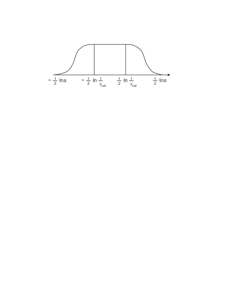
Figure 17: Rapidity plateau in two-jet events.

The average particle multiplicity in the selected two-jet sample is smaller than in an unbiased sample. The modification due to the bias is similar to the suppression from a Sudakov form factor. It is formally ${\cal O}(\alpha_{S})$, but it also contains a factor $\ln^{2}(s/p_{\perp}^{2})$. Thus, it is small for large $p_{\perp}$-values but it becomes significant for smaller $p_{\perp}$. This clearly demonstrates that the multiplicity in this restricted case depends on two scales, $\sqrt{s}$ and $p_{\perp{\rm cut}}$. The $p_{\perp}$ of an emitted gluon is related to the virtual mass of the radiating parent quark. Therefore, the two scales $\sqrt{s}/2$ and $p_{\perp{\rm cut}}$ represent the energy and virtuality of the quark and antiquark initiating the jets.

Though the leading-logarithmic result in Eq. (7.4) describes qualitatively an impact of the bias, for a quantitative analysis an account of the subleading effects may be required. These subleading corrections were calculated $\!{}^{{\bf?}}$ where the MLLA formula for the biased two-jet-event multiplicity was presented as

$$N_{q\bar{q}}(L,\kappa_{\rm cut})\;\approx\;N_{q\bar{q}}(\kappa_{\rm cut}+c_{q})\>+\>(L-\kappa_{\rm cut}-c_{q})\>N_{q\bar{q}}^{\prime}(\kappa_{\rm cut}+c_{q});\quad c_{q}\;=\;\frac{3}{2}.$$ (172)

The results from the ARIADNE Monte Carlo are demonstrated $\!{}^{{\bf?}}$ to be in good agreement with the prediction of Eq. (172).

Let us return now to the three-jet-event case. As was already discussed, in the large-$N_{C}$ limit the emission of softer gluons from a $q\bar{q}g$ system corresponds to two antennas-dipoles which emit gluons independently. If a gluon jet is resolved with the transverse momentum $p_{\perp}$, this imposes a constraint on the emission of sub-jets from the two antennas. Thus, the contribution from each antenna is determined by an expression like Eqs. (7.4,172).

An essential issue concerns the definition of the jet resolution scale $p_{\perp}$ for three-jet events. In the Lund dipole approach $\!{}^{{\bf?},{\bf?},{\bf?}}$ $p_{\perp}$ is defined as

$$p_{\perp{\rm Lu}}^{2}\;=\;\frac{4(p_{+}\cdot p_{1})(p_{-}\cdot p_{1})}{s},$$ (173)

c.f. Eqs. (146, 166).

These two $p_{\perp}$-definitions agree for soft gluons but deviate for harder gluons. While $p_{\perp{\rm Lu}}$ is always bounded by $\sqrt{s}/2$ the scale parameter $p_{1\perp}$ in Eq. (166) has no kinematic upper limit in the massless case. For hard gluons $p_{\perp{\rm Lu}}$ is of the same order as the parent quark virtuality. It was shown $\!{}^{{\bf?}}$ that the ${\cal O}(\alpha_{S}^{2})$ matrix elements are well described if $p_{\perp{\rm Lu}}$ is chosen as an ordering parameter in the perturbative branching. Therefore, it looks natural to assume $\!{}^{{\bf?},{\bf?}}$ that the constraint on further emissions is described by the identification $p_{\perp{\rm cut}}=p_{\perp{\rm Lu}}$. The multiplicity in a $qg$-dipole with restricted $p_{\perp}$ can be described, analogously to the $q\bar{q}$-case, as two forward regions and a central plateau.

We conclude this subsection by focusing on the three-jet configurations obtained by iterative clustering until exactly three jets remain, without a specified resolution scale, where, hence, the constraint on sub-jet $p_{\perp}$ is described by $p_{\perp{\rm cut}}=p_{\perp{\rm Lu}}$. This allows us to avoid ‘biasing’ the gluon jet sample, which makes this selection procedure convenient for extracting the unbiased $gg$-multiplicity. $\!{}^{{\bf?}}$ This strategy is chosen in the recent DELPHI analysis  $\!{}^{{\bf?},{\bf?}}$ while each event is clustered to precisely three jets.

By clustering each event to three jets one gets $\!{}^{{\bf?}}$ for the multiplicity in three-jet events (c.f. Eqs. (165–168))

$$N_{q\bar{q}g}\;=\;N_{q\bar{q}}(L_{q\bar{q}},\kappa_{\rm Lu})\>+\>\frac{1}{2}\>N_{gg}(\kappa),$$ (174)

with

$$L_{q\bar{q}} = \ln\frac{2(p_{+}\cdot p_{-})}{\Lambda^{2}},\quad\kappa_{\rm Lu}\;=\;\ln\frac{4(p_{+}\cdot p_{1})(p_{-}\cdot p_{1})}{s\Lambda^{2}},$$

$$\kappa = \ln\frac{2(p_{+}\cdot p_{1})(p_{-}\cdot p_{1})}{(p_{+}\cdot p_{-})\Lambda^{2}}\;=\;\ln\frac{p_{1_{\perp}}^{2}}{\Lambda^{2}}.$$

An alternative expression for $N_{q\bar{q}g}$ is given as $\!{}^{{\bf?}}$

$$N_{q\bar{q}g}\;=\;N_{q\bar{q}}(L,\kappa_{\rm Lu})\>+\>\frac{1}{2}\>N_{gg}(\kappa_{\rm Lu}).$$ (176)

Note that the consistency between Eqs. (174) and (176) follows from the fact that the total rapidity range in the $qg$ and $\bar{q}g$-dipoles,

$$L_{qg}\>+\>L_{g\bar{q}}\;=\;\ln\frac{2(p_{+}\cdot p_{1})}{\Lambda^{2}}\>+\>\ln\frac{2(p_{-}\cdot p_{1})}{\Lambda^{2}},$$ (177)

can be described in two different ways by the equalities

$$L_{qg}+L_{g\bar{q}}\;=\;L_{q\bar{q}}+\kappa\;=\;L\>+\>\kappa_{\rm Lu}.$$ (178)

Let us emphasize that due to QCD coherence the argument in $N_{gg}$ is $p_{1\perp}^{2}$ in (174) and $p_{1\perp{\rm Lu}}^{2}$ in (176) and not $(2p_{\perp})^{2}$ as one would naively expect. The difference between the results of Eqs. (174) and (176) arises from the subleading corrections (for example, recoil effects) which are not controllable within this framework. $\!{}^{{\bf?}}$

Formally the bias is related to order $\alpha_{S}$ effects, and while it practically does not affect the gluon piece it can be important for the $q\bar{q}$-contribution. Selecting events with comparatively large values of $p_{\perp}$, where the bias is not essential, we arrive at the old result $\!{}^{{\bf?}}$ (c.f. Eq. (165))

$$N_{q\bar{q}g}\;=\;\left[N_{q\bar{q}}(L_{q\bar{q}})\>+\>\frac{1}{2}\>N_{gg}(\kappa)\right]\>\left[1+{\cal O}(\alpha_{S})\right].$$ (179)

The effect of the bias becomes more and more important for smaller values of $p_{\perp{\rm cut}}$. On the other hand, $\!{}^{{\bf?}}$ the bias is negligible if one selects gluon system recoiling against two quark jets in the same hemisphere.

7.5 Experimental Studies of Three-Jet Events

In this subsection we focus mainly on the new experimental evidence of the inter-jet color coherence effects from the analyses of the LEP-1 data, also discussed in recent reviews. $\!{}^{{\bf?},{\bf?},{\bf?},{\bf?},{\bf?}}$ The main lesson from the recent impressive studies is that now we have (quite successfully) entered the stage of quantitative tests of the details of color drag phenomena. Owing to the massive LEP-1 statistics, one can perform a very detailed study allowing to test even some subtle features of the theoretical expectations.

Let us mention a few new facts concerning comparison with the analytical QCD predictions. DELPHI $\!{}^{{\bf?}}$ have performed the first quantitative verification of the perturbative prediction $\!{}^{{\bf?}}$ for the ratio $R_{\gamma}$

$$R_{\gamma}\;=\;\frac{N_{q\bar{q}}(q\bar{q}g)}{N_{q\bar{q}}(q\bar{q}\gamma)}$$ (180)

of the particle population densities in the interquark valley in the $e^{+}e^{-}\rightarrow q\bar{q}g$ and $e^{+}e^{-}\rightarrow q\bar{q}\gamma$ events. For a clearer quantitative analysis a comparison was performed for the $Y$-shaped symmetric events using the double-vertex method for the $q$-jet tagging. The ratio $R_{\gamma}$ of the charged particle flows in the $q\bar{q}$ angular interval [$35^{\circ},115^{\circ}$] was found to be

$$R_{\gamma}^{\exp}\;=\;0.58\>\pm\>0.06.$$ (181)

This value is in fairly good agreement with the expectation following from Eqs. (7.2) and (142) at $N_{C}=3$, for the same angular interval

$$R_{\gamma}^{th}\;\approx\;\frac{0.65N_{C}^{2}-1}{N_{C}^{2}-1}\;\approx\;0.61.$$ (182)

(Note that this ratio is slightly larger than the one predicted for Mercedes-type events in (143)). The string/drag effect is quantitatively explained by the perturbative prediction and the above ratio does not appear to be affected by hadronization effects in an essential way.

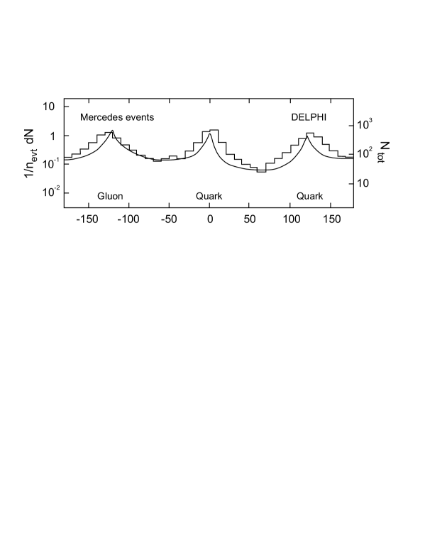
Figure 18: Charged particle flow in $q\bar{q}g$-events $\!{}^{{\bf?}}$ in comparison with analytical prediction. $\!{}^{{\bf?}}$

Another DELPHI result $\!{}^{{\bf?}}$ concerns the analysis of the threefold-symmetric $e^{+}e^{-}\rightarrow q\bar{q}g$ events using the double-vertex tagging method. It is shown that the string/drag effect is clearly present in these fully symmetric events and it cannot be an artefact due to kinematic selections. The azimuthal-angle dependence of particle density in the event plane is shown in Fig. 18. Quantitatively, comparing the minima located at $\pm[50^{\circ},70^{\circ}]$, the particle population ratio $R_{g}=N_{qg}/N_{q\bar{q}}$ in the $q-g$ and $q-\bar{q}$ valleys is found to be

$$R_{g}^{\exp}\;=\;2.23\>\pm\>0.37.$$ (183)

This is to be compared with the asymptotic prediction $R_{g}=2.46$ for projected rates at central angles, whereas for the above angular interval one finds $\!{}^{{\bf?},{\bf?}}$

$$R_{g}^{th}\;\approx\;2.4$$ (184)

in good agreement with the experimental value. The number (184) was obtained from the prediction for the full angular distribution $\!{}^{{\bf?}}$ (see subsection 2.3) which is also displayed in Fig. 18 with the normalization adjusted. The calculation takes into account both the inside-jet and inter-jet coherence. As can be seen, the relative depth of the two valleys between the jets is well reproduced. Also reasonable is the distribution around the gluon jet direction. On the other hand, more particles than expected are found within the quark jets. In part this is a consequence of using in the calculation the asymptotic value 4/9 for $1/r$, which, as we have already discussed, is approached rather slowly from above. Despite these shortcomings, the main effect, the ratio $R_{g}$ of particle densities in the valleys between the two types of jets, has been correctly predicted by the analytical calculations.

Another prediction concerns the beam-energy dependence. At a higher energy the angular density in Fig. 18 gets essentially multiplied by an overall factor: $\!{}^{{\bf?}}$ the particle density in between the jets rises at a rate comparable to the density within the jets.

An instructive test of the inter-jet coherence can be performed when studying the particle flow in the direction transverse to the 3-jet event plane. $\!{}^{{\bf?}}$ Consider the radiation of a soft gluon perpendicular to the plane of a 3-jet $q\overline{q}g$ event. This radiation can be obtained from (138) where the contribution from one antenna is simply $(\widehat{ij})=1-\cos\Theta_{ij}$. The ratio $R_{\perp}=dN^{q\overline{q}g}/dN^{q\overline{q}}$ of soft perpendicular radiation in three and two-jet events is obtained as $\!{}^{{\bf?}}$

$$R_{\perp}=\frac{N_{C}}{4C_{F}}[2-\cos\Theta_{1+}-\cos\Theta_{1-}-\frac{1}{N_{C}^{2}}(1-\cos\Theta_{+-})].$$ (185)

In the large $N_{C}$ limit we have just the superposition of two dipoles with contribution $\sim 1-\cos\Theta_{1q}$. Note the limiting cases $R_{\perp}=1$ for collinear primary gluon emission and the proper $gg$ limit $R_{\perp}=N_{C}/C_{F}$ for the configuration with parallel $q\overline{q}$ ($\Theta_{+-}=0)$ recoiling against the gluon.

DELPHI $\!{}^{{\bf?}}$ have presented the first results on the particle yield in the transverse direction for the $Y$-shaped symmetric $q\bar{q}g$-events. Fig. 19 shows the multiplicity within the cone with the fixed opening angle of $30^{\circ}$ perpendicular to the event plane. The abscissa is the angle $\Theta_{1}$ between the low-energy jets (the non-leading $q$-jet and the gluon). The plotted curve corresponds to the perturbative prediction from Eq. (185) using $\Theta_{1+}=\Theta_{+-}=\pi-\Theta_{1}/2$ and $\Theta_{1-}=\Theta_{1}$ with the normalization left free. The rise of particle flow observed for increasing opening angle $\Theta_{1}$ signals an increase of the “effective color charge” corresponding to a transition from a $q\overline{q}$ to a $gg$ type antenna. The experimental data prove to be in a quite good agreement with the perturbative predictions, providing a new test of the analytical results independent of the hadronization models.

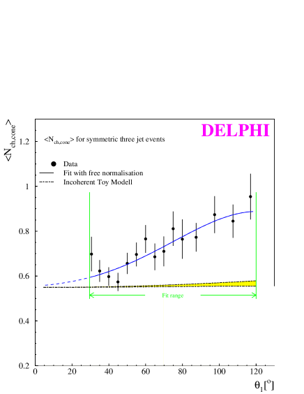
Figure 19: Multiplicity within a $30^{\circ}$-cone perpendicular to three-jet-event plane as a function of the event topology. $\!{}^{{\bf?}}$ The curve represents the perturbative prediction (185).

Of special interest is also the measurement of the yield of particles perpendicular to the production plane in the low momentum range. $\!{}^{{\bf?}}$ Within the perturbative scenario the very soft particle production should be sensitive again only to the color charge topology of the primary emitters. It looks quite challenging to test whether the angular dependence of the particle yield given by Eq. (185) holds downwards up to small momenta $p\sim Q_{0}$.

If one allows for arbitrary three-jet kinematic configurations, new information can be obtained about the evolution of the event portrait with the variation of toplogy, see previous subsection. ALEPH, $\!{}^{{\bf?}}$ DELPHI $\!{}^{{\bf?},{\bf?},{\bf?},{\bf?}}$ and OPAL $\!{}^{{\bf?}}$ have convincingly demonstrated that, in agreement with the QCD radiophysics, the event multiplicity in three-jet events depends both on the jet energies and on the angles between the jets. These results clearly show the predicted toplogical dependence of jet properties.

Recently DELPHI $\!{}^{{\bf?}}$ have reported the new results on the total charged particle multiplicity in $Y$-shaped three-jet events. A crucial point in the DELPHI analysis  $\!{}^{{\bf?},{\bf?}}$ is that each event is clustered to precisely three jets. This allows to determine $N_{q\bar{q}g}$ as a function of the opening angle, $\Theta_{1}$, between the low-energy jets and to extract the ‘unbiased’ $gg$-multiplicity, $N_{gg}$. Recall that in symmetric $Y$-events there are only two scale parameters, $\sqrt{s}=M_{Z}$ and $\Theta_{1}$, so the event-topology dependence can be expressed as a function of $\Theta_{1}$ only, assuming that the leading jet is not the gluon jet, which is true for most cases. A comparison is performed $\!{}^{{\bf?}}$ with analytical results based on Eqs. (174, 176). The values of $N_{q\bar{q}}$ entering the expressions (174, 176) via Eq. (172) are extracted from the existing data on the energy dependence of $N_{e^{+}e^{-}}$, using the standard parametrizations. $\!{}^{{\bf?}}$

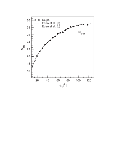
Figure 20: Fits of Eqs. (174)(a) and Eq. (7.4)(b) to the data. The full points depict the range of the fit. $\!{}^{{\bf?}}$

Fig 20 $\!{}^{{\bf?}}$ shows the results of comparison with the predictions of Eqs. (174) and (176). In both cases one finds a good agreement with the data. DELPHI analysis clearly demonstrates that Eqs. (174, 176) fit the data in the wide $\Theta_{1}$-range better than the ‘unbiased’ Eq. (179).

7.6 Collective Phenomena in High-$p_{\perp}$ Hadronic Reactions

Color coherence leads to a rich diversity of interference drag-effects in high-$p_{\perp}$ multi-jet events in hadronic collisions (see, for example, Refs. 128,146,155,179, 161,162) and in $\gamma p$ and DIS processes (see, for example, Refs. 59,180,181). The analysis of collective drag phenomena in these processes is considerably more subtle than in $e^{+}e^{-}$ annihilation due to the presence of colored constituents in both initial and final states.

Recall that during a hard interaction, color is transferred from one parton to another and the color-connected partons act as color antennas, with interference effects taking place in the initial or final states, or between the initial and final states. Radiation from the incoming and outgoing partons forms jets of hadrons around the direction of these colored emitters. The soft gluon radiation pattern accompanying a hard partonic system can be represented, to leading order in $1/N_{C}$, as a sum of contributions corresponding to the color-connected partons. $\!{}^{{\bf?},{\bf?}}$ In hadronic high-$p_{\perp}$ reactions by varying the experimental conditions (triggers) one may separate the dominant partonic subprocesses and switch from one subprocess to another. Recall also that the length and height of the hadronic “plateau” depend here on different parameters: the length is determined by the total energy of the collision, and the height and the plateau structure depend on the hardness of the process governed, as a rule, by the transverse energy-momentum transfer. Thus, information becomes available that is inaccessible in $e^{+}e^{-}$ annihilation where both energy and hardness were given by the value of $\sqrt{s}$. Therefore, the high-$p_{\perp}$ hadronic collisions provide us with a very prospective laboratory for the detailed studies of the color-related phenomena.

As a simple illustrative example let us consider the topology of events, resulting from the high-$p_{\perp}$ $qq$-scattering $\!{}^{{\bf?},{\bf?}}$ which has been studied recently in detail. $\!{}^{{\bf?}}$

$$-\hat{t}\>\sim\>\hat{s}\;=\;x_{1}\cdot x_{2}\>s\quad\quad(x_{1},x_{2}\sim 1).$$ (186)

In this case the two crossing processes shown in Fig. 21(a) and 21(b) have approximately equal probabilities. However, each of them has its own color topology, and therefore, specific particle flows, as schematically shown in Fig. 21(c) and 21(d).

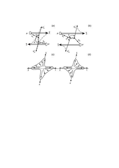
Figure 21: Color antennas for two crossing subprocesses of $qq$-scattering (a,b) and the drawings of the corresponding hadronic flows (c,d).

For the subprocess of Fig. 21(a) the soft particle radiation pattern is

$$\quad\quad\quad\quad\quad\quad\quad\frac{4\pi dN^{q_{1}q_{2}}}{d\Omega_{\vec{n}}}\;=\;\frac{C_{F}}{N_{C}}\>N_{g}^{\prime}\left(\ln\frac{E}{\Lambda}\right)$$

(187)

$$\times\left\{(\widehat{14})+(\widehat{23})\>+\>\frac{1}{2N_{C}C_{F}}\>\left(2[(\widehat{12})+(\widehat{34})]-(\widehat{14})-(\widehat{23})-(\widehat{13})-(\widehat{24})\right)\right\},$$

where antenna $\widehat{ij}$ is given by Eq. (139). In full analogy with the discussions of the drag effect in subsection 2.2 one may say that the leading contribution (the first term in (7.6)) has the structure of the sum of two independent $q\bar{q}$-antennas $(\widehat{14})$ and $(\widehat{23})$. This fact also can be mimicked by means of the topological picture of the Lund string model. Let us emphasize that in our case to each contribution (single antenna) a dynamical distribution corresponds which takes into account the effects of cascade multiplication. Furthermore, the perturbative approach permits one to control not only the leading color contribution, but also the ${\cal O}(1/N_{C})$ corrections.

The complete set of antenna patterns for various parton scattering subprocesses for arbitrary $N_{C}$ is listed in. $\!{}^{{\bf?}}$

It has been known for a long time $\!{}^{{\bf?},{\bf?}}$ that an especially bright color interference effect arises in the case of large-$E_{T}$ production of color singlet objects, for instance, in $V+$ jet events (with $V=\gamma,W^{\pm}$ or $Z$). The hadronic antenna patterns for such processes are entirely analogous to that in the celebrated string-drag effect in $e^{+}e^{-}\rightarrow q\bar{q}g$ events.

Recently the first (very impressive) data on $W+$ jet production from D0 $\!{}^{{\bf?},{\bf?}}$ have become available. The color-coherence effects are clearly seen and these studies have a very promising future. They may play the same role for hadron colliders as the important series of results on inter-jet studies at $e^{+}e^{-}$ colliders. The quantitative predictions were presented $\!{}^{{\bf?}}$ for color interference phenomena in the distribution of soft particles and jets in $V+$ jet production at hadron colliders, in particular the Tevatron $\sqrt{s}=1.8~{}{\rm TeV}~{}p\bar{p}$ collider. There are two leading-order processes, $q\bar{q}\rightarrow Vg$ and $qg\rightarrow Vq$. Each has its own distinctive antenna pattern. In principle, the antenna pattern could be used as a ‘partonometer’ to identify the dominant scattering process.

Omitting the CKM factors for clarity, the matrix elements squared for the lowest-order processes (for the case $V=W$) can be written as

$$\overline{\sum}|{\cal M}|^{2}\left(q(p_{1})\bar{q}(p_{2})\rightarrow W(p_{3})g(p_{4})\right) = \frac{g_{s}^{2}g_{W}^{2}}{4}\left(1-\frac{1}{N_{C}^{2}}\right)\frac{t^{2}+u^{2}+2sM_{W}^{2}}{tu},$$

$$\overline{\sum}|{\cal M}|^{2}\left(q(p_{1})g(p_{2})\rightarrow W(p_{3})q(p_{4})\right) = \frac{g_{s}^{2}g_{W}^{2}}{4}\>\frac{1}{N_{C}}\>\frac{t^{2}+s^{2}+2uM_{W}^{2}}{-ts},$$

where $s=(p_{1}+p_{2})^{2},t=(p_{1}-p_{3})^{2}$ and $u=(p_{1}-p_{4})^{2}$. In the soft-gluon approximation, the corresponding $2\rightarrow 3$ matrix elements are

$$\overline{\sum}|{\cal M}|^{2}(q\bar{q}\rightarrow Wg(g)) = g_{s}^{2}N_{C}\left([14]+[24]-\frac{1}{N_{C}^{2}}\>[12]\right)\>\overline{\sum}|{\cal M}|^{2}(q\bar{q}\rightarrow Wg)$$

$$\overline{\sum}|{\cal M}|^{2}(qg\rightarrow Wq(g)) = g_{s}^{2}N_{C}\left([12]+[24]-\frac{1}{N_{C}^{2}}\>[14]\right)\>\overline{\sum}|{\cal M}|^{2}(qg\rightarrow Wq)$$

with

$$[ij]\;\equiv\;\frac{p_{i}\cdot p_{j}}{p_{i}\cdot k\>p_{j}\cdot k}\;=\;\frac{1}{E_{k}^{2}}\>(\widehat{ij}).$$ (190)

Note that for these processes, the effect of the soft gluon emission is simply to multiply the lowest-order matrix elements squared by an overall factor consisting of three different antennas, defined according to (7.6), one of which is suppressed in the large $N_{C}$ limit. This structure is universal for any electroweak boson + jet production, i.e. $V=W^{\pm},Z^{0},\gamma,\gamma^{*}$.

It is worthwhile to mention that the study of soft radiation pattern accompanying dijet photoproduction can provide a new tool to distinguish the so-called direct and resolved mechanisms. $\!{}^{{\bf?},{\bf?}}$ Of special interest here is the measurement of the soft particle yield perpendicular to the reaction plane. $\!{}^{{\bf?},{\bf?}}$

Inter-jet color coherence effects were successfully studied by both the CDF and D0 Collaborations in $p\bar{p}$ collisions at the Fermilab Tevatron Collider. $\!{}^{{\bf?},{\bf?},{\bf?}}$ The experimental results look rather promising. Thus, the measurements $\!{}^{{\bf?},{\bf?}}$ of the spatial correlations between the softer third jet and the second leading-$E_{T}$ jet in $p\bar{p}\rightarrow$ 3 jet $+X$ events has clearly demonstrated the presence of initial-to-final interference effects in $p\bar{p}$ interactions.

In the most direct way the drag-effect signal is extracted in the recent D0 analysis $\!{}^{{\bf?}}$ of $W+$ jet events by comparing the soft particle angular distributions around the colorless $W$ boson and opposing leading-$E_{T}$ jet in the same event. In this study the $W$ boson provides a template against which the soft particle pattern around the jet can be compared. Such comparison reduces the sensitivity to various biases that may be present in the vicinity of both the $W$ boson and the jet.

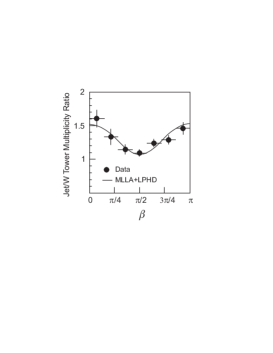
Figure 22: Comparison of the jet/$W$ multiplicity ratio from data to the MLLA-LPHD prediction $\!{}^{{\bf?}}$

Inter-jet coherence effects clearly manifest themselves as an enhancement of soft particle radiation around the tagged jet in the event plane (the plane defined by the direction of the $W$ boson and the beam axis) relatively to the transverse plane when compared with the particle production around the $W$ boson. This is illustrated in Fig. 22 which shows D0 results for the jet/$W$ particle flow ratio as a function of the azimuthal angle $\beta$ together with the perturbative expectation based on MLLA and LPHD. $\!{}^{{\bf?}}$ The analytical prediction proves to be in good quantitative agreement with the data, thus providing new evidence supporting the LPHD picture.

8 Conclusions

Perturbative QCD proves to be very successful in its applications to multiparticle production in hard processes. Still, the problem of the soft limit of the theory and of color confinement is not solved. Therefore, at present stage hadroproduction phenomena cannot be derived solely from the perturbation theory without additional model-dependent assumptions. The complexity of the existing popular models requires Monte-Carlo methods to derive their predictions.

In this review we have concentrated on the question of the extent to which the semisoft phenomena in multiparticle production in hard processes reflect the properties of the perturbative QCD cascades.

During the last years the experiments have collected exceedingly rich new information on the dynamics of hadronic jets — the footprints of QCD partons. New QCD physics results from LEP2, TEVATRON and HERA continue to pour out shedding light on various aspects of hadroproduction in multi-jet events. The existing data convincingly show that the analytical perturbative approach to QCD jet physics is in a remarkably healthy shape.

The key concept of this approach is the hypothesis of local parton- hadron duality, according to which the parton cascade can be evolved down to a low virtuality scale of the order of the hadronic masses, where the conversion of partons into hadrons occurs. Therefore it is the physics of QCD branching which governs the gross features of the jet development.

In particular, the perturbative universality of jets appearing in different hard processes is nicely confirmed. Moreover, the data demonstrate that the transition between the perturbative and non-perturbative stages of jet evolution is quite smooth, and that the bright color coherence phenomena successfully survive the hadronization stage.

LEP1 proves to be a priceless source of information on the QCD dynamics. It has benefited from the record statistics and the substantial lack of background. We have learned much interesting physics, but there is still a need for further refined analyses of the data recorded at LEP1.

The programs of QCD studies at the LHC and at a future linear $e^{+}e^{-}$ collider look quite promising. The semisoft QCD physics steadily becomes one of the important topics for investigation in the TEVATRON and HERA experiments.

Concluding this review let us emphasize once more that, of course, there is no mystery within the perturbative QCD framework. One is only supposed to perform the calculational routine properly. So it is entirely unremarkable that the quantum mechanical interference effects should be observed in the perturbative results. Of real importance is that the experiment demonstrates that the transformer between the perturbative and non-perturbative phases acts very smoothly. This message could (some day) shed light on the mechanism of color confinement.

References

References

- [1] B.L. Ioffe, V.A. Khoze and L.N. Lipatov, Hard Processes, Vol. 1, (North Holland, Amsterdam, 1984).
- [2] R. P. Feynman, Photon-Hadron Interactions, (Benjamin, N.Y., 1972).
- [3] J.D. Bjorken and E.A. Paschos, Phys. Rev. 185, 1975 (1969).
- [4] R. F. Schwitters et al., Phys. Rev. Lett. 35, 1320 (1975); G. G. Hanson et al., Phys. Rev. Lett. 35, 1609 (1975).
- [5] H. Fritzsch and M. Gell-Mann, in Proc. XVI Int. Conf. on High Energy Physics, eds. J.D. Jackson and A. Roberts, Vol. 2, p. 135 ( Batavia 1972); H. Fritzsch, M. Gell-Mann and H. Leutwyler, Phys. Lett. B 47, 365 (1973).
- [6] TASSO Collaboration, R. Brandelik et al., Phys. Lett. B 86, 243 (1979); B 94, 436 (1980); MARK J Collaboration, D. P. Barber et al., Phys. Rev. Lett. 43, 830 (1979); PLUTO Collaboration, Ch. Berger et al., Phys. Lett. B 86, 418 (1979); JADE Collaboration, W. Bartel et al., Phys. Lett. B 91, 142 (1980).
-
[7]
D. Gross and F. Wilczek, Phys. Rev. Lett. 30, 1343 (1973);
H.D. Politzer, Phys. Rev. Lett. 30, 1346 (1973). - [8] S. Bethke, “ Determination of the QCD coupling ”, hep-ex/0004021.
-
[9]
G. Marchesini and B.R. Webber,
Nucl. Phys. B 238, 1 (1984);
310, 461 (1988);
G. Marchesini, B.R. Webber, G. Abbiendi, I.G. Knowles, M.H. Seymour, and L. Stanco, Comp. Phys. Comm. 67, 465 (1992); HERWIG version 5.9, hep-ph/9607393. -
[10]
T. Sjöstrand,
Comp. Phys. Comm. 39, 347 (1986);
T. Sjöstrand and M. Bengtsson, Comp. Phys. Comm. 43, 367 (1987);
T. Sjöstrand, CERN preprint, CERN-TH 6488/92. -
[11]
L. Lönnblad, in Physics at HERA, Vol. 3
(1991) 1440;
L. Lönnblad, Comp. Phys. Comm. 71, 15 (1992) - [12] B. Andersson, G. Gustafson, G. Ingelman and T. Sjöstrand, Phys. Rep. 97, 31 (1983).
- [13] Yu. Dokshitzer, “Perturbative QCD and Power Corrections”, Int. Conf. Frontiers of matter, Blois, France, June 1999, hep-ph/9911299.
- [14] Ya.I. Azimov, Yu.L. Dokshitzer, V.A. Khoze and S.I. Troyan, Z. Phys. C 27, 65 (1985); ibid, 31, 213 (1986).
- [15] Yu.L. Dokshitzer, V.A. Khoze, A.H. Mueller and S.I. Troyan, Basics of Perturbative QCD, ed. J. Tran Thanh Van (Editions Frontiéres, Gif-sur-Yvette, 1991).
- [16] R.K. Ellis, W.J. Stirling and B.R. Webber, QCD and Collider Physics (Cambridge University Press, Cambridge, 1996).
- [17] V.A. Khoze and W. Ochs, Int. J. Mod. Phys. A 12, 2949 (1997).
- [18] I.G. Knowles, G.D. Lafferty, J. Phys. G 23, 731 (1997).
-
[19]
F. Bloch, A. Nordsieck,
Phys. Rev. 52, 54 (1937);
D.R. Yennie, S.C. Frautschi, M. Suura, Ann. Phys. 13, 319 (1961). - [20] G. Sterman and S. Weinberg, Phys. Rev. Lett. 39, 1436 (1977).
- [21] W. J. Stirling in Proceedings of the Durham Workshop on Jet Studies at LEP and HERA; J. Phys. G 17, 1567 (1991).
- [22] T. Sjöstrand, Comp. Phys. Comm. 28, 229 (1983).
- [23] N. Brown and W.J. Stirling, Phys. Lett. B 252, 657 (1990); Z. Phys. C 53, 629 (1992).
- [24] S. Catani, Yu.L. Dokshitzer, M. Olsson, G. Turnock and B.R. Webber, Phys. Lett. B 269, 432 (1991).
- [25] S. Bethke, Z. Kunszt, D.E. Soper and W.J. Stirling, Nucl. Phys. B 370, 310 (1992).
-
[26]
JADE Collaboration, W. Bartel et al.,
Z. Phys. C 33, 23 (1986);
S. Bethke et al., Phys. Lett. B 213, 235 (1988). - [27] Yu. L. Dokshitzer, G.D. Leder, S. Moretti and B.R. Webber, JHEP 9708, 1 (1997).
- [28] M.H. Seymour, “Jets in Hadron Collisions”, XXXVth Rencontre de Moriond, March 2000, hep-ph/0007051.
- [29] J. D. Bjorken, Phys. Rev. 179, 1547 (1969).
- [30] SLAC-MIT Collaboration, G. Miller et al., Phys. Rev. D 5, 528 (1972).
-
[31]
H. Georgi and H.D. Politzer, Phys. Rev. D 9, 416 (1974);
D.J. Gross and F. Wilczek, Phys. Rev. D 9, 980 (1974). - [32] V.N. Gribov and L.N. Lipatov, Sov. J. Nucl. Phys. 15, 438 (1972); ibid, 675; L.N. Lipatov, Sov. J. Nucl. Phys. 20, 94 (1975).
- [33] G. Altarelli and G. Parisi, Nucl. Phys. B 126, 298 (1977).
- [34] Yu.L. Dokshitzer, Sov. Phys. JETP 46, 641 (1977).
- [35] C.H. Llewellyn Smith, Acta. Phys. Austr. Supp. 19, 331 (1978).
- [36] Yu.L. Dokshitzer, Y.L. Dyakonov and S.I. Troyan, Phys. Rep. C 58, 269 (1980).
-
[37]
G. Curci, W. Furmanski and R. Petronzio,
Nucl. Phys. B 175, 27 (1980);
W. Furmanski and R. Petronzio, Phys. Lett. B 97, 437 (1980). - [38] S. Pokorski, Gauge Field Theories, (Cambridge University Press, Cambridge, 2000).
- [39] J.C. Collins and D.E. Soper, Ann. Rev. Nucl. Part. Sci 37, 383 (1987).
- [40] R.K. Ellis et al., Nucl. Phys. B 152, 285 (1979).
- [41] C.T.C. Sachrajda in Tahoe Multiparticle Dynamics, ed. J. Gunion (University of Davies, Davies, 1983) 415.
- [42] J. Wosiek and K. Zalewski, Acta Phys. Polon. B 10, 667 (1979).
- [43] V.V. Sudakov, Sov. Phys. JETP 3, 65 (1956).
- [44] A. H. Mueller, Nucl. Phys. B 213, 85 (1983); erratum ibid, 241, 141 (1984).
- [45] B.I. Ermolayev and V. S. Fadin, JETP Lett. 33, 285 (1981)
- [46] A.H. Mueller, Phys. Lett. B 104, 161 (1981).
- [47] A. E. Chudakov, Izv. Akad. Nauk SSSR, Ser. Fiz. 19, 650 (1955).
- [48] W. Furmanski, R. Petronzio and S. Pokorski, Nucl. Phys. B 155, 253 (1979).
- [49] A. Bassetto, M. Ciafaloni and G. Marchesini, Nucl. Phys. B 163, 477 (1980).
- [50] Yu.L. Dokshitzer, V.S. Fadin and V.A. Khoze, Phys. Lett. B 115, 242 (1982); Z. Phys. C 15, 325 (1982).
- [51] A. Bassetto, M. Ciafaloni, G. Marchesini and A.H. Mueller, Nucl. Phys. B 207, 189 (1982).
- [52] Yu.L. Dokshitzer and S.I. Troyan, in Proc. 19th Winter School of the LNPI, Vol. 1, p.144; Leningrad preprint LNPI-922 (1984).
- [53] Yu.L. Dokshitzer, V.A. Khoze and S.I. Troyan in Advanced Series on Directions in High Energy Physics – Perturbative Quantum Chromodynamics, ed. A.H. Mueller (World Scientific, Singapore, 1989), V. 5, p. 241.
- [54] A. Bassetto, M. Ciafaloni and G. Marchesini, Phys. Rep. C 100, 201 (1983).
- [55] Yu.L. Dokshitzer, V.S. Fadin and V.A. Khoze, Z. Phys. C 18, 37 (1983).
- [56] V.S. Fadin, Sov. J. Nucl. Phys. 37, 245 (1983).
-
[57]
D. Amati and G. Veneziano,
Phys. Lett. B 83, 87 (1979);
A. Bassetto, M. Ciafaloni and G. Marchesini, Phys. Lett. B 83, 207 (1979); G. Marchesini, L. Trentadue and G. Veneziano, Nucl. Phys. B 181, 335 (1981). - [58] S. Lupia, W. Ochs, Phys. Lett. B 365, 339 (1996); Eur. Phys. J. C 2, 307 (1998).
- [59] V.A. Khoze, S. Lupia, W. Ochs, Phys. Lett. B 386, 451 (1996); Eur. Phys. J. C 5, 77 (1998).
- [60] Ya.I. Azimov, Yu.L. Dokshitzer and V.A. Khoze, in Proceedings of the XVII Winter School of the LNPI, Vol. I, p.162, (Leningrad, 1982).
- [61] W. Ochs and T. Shimada, in Proc. XXIX Int. Symp. QCD & Multiparticle Production (ISMD99), to appear, Brown Univ., Providence, RI, USA, Aug. 1999, hep-ph/9911240.
- [62] Yu.L. Dokshitzer and M. Olsson, Nucl. Phys. B 396, 137 (1993).
- [63] B.R. Webber, Phys. Lett. B 143, 501 (1984).
- [64] Ya.I. Azimov, Yu.L. Dokshitzer, V.A. Khoze and S.I. Troyan, Phys. Lett. B 165, 147 (1985); Sov. J. Nucl. Phys. 43, 95 (1986).
- [65] S.J. Brodsky and J.F. Gunion, Phys. Rev. Lett. 37, 402 (1976).
- [66] K. Konishi, A. Ukawa and G. Veneziano, Nucl. Phys. B 157, 45 (1979).
- [67] E.D. Malaza, B.R. Webber, Phys. Lett. B 149, 501 (1984); Nucl. Phys. B 267, 702 (1986).
- [68] J.B. Gaffney and A.H. Mueller, Nucl. Phys. B 250, 109 (1985).
- [69] I.M. Dremin and V.A. Nechitailo, Mod. Phys. Lett. A 9, 1471 (1994).
- [70] A. Capella, I.M. Dremin, J.W. Gary, V.A. Nechitailo and J. Tran Thanh Van, Phys. Rev. D 61, 074009 (2000).
- [71] I.M. Dremin and J.W. Gary, “Hadron Multiplicities”, hep-ph/0004215.
- [72] A.M. Polyakov, Sov. Phys. JETP 32, 296 (1971); ibid 33, 850 (1971).
- [73] S. Catani, Yu. L. Dokshitzer, F. Fiorani and B. R. Webber, Nucl. Phys. B 377, 445 (1992).
- [74] S. Lupia and W. Ochs, Phys. Lett. B 418, 214 (1998).
- [75] S. Lupia and W. Ochs, Nucl. Phys. B (Proc. Suppl.) 64, 74 (1998).
- [76] DELPHI Collaboration, P. Abreu et al., Phys. Lett. B 416, 233 (1998).
- [77] OPAL Collaboration, G. Abbiendi et al., hep-ex/0002012, submitted to Eur. Phys. J. C.
- [78] L3 Collaboration, O. Adriani et al., Phys. Lett. B 284, 471 (1992).
- [79] OPAL Collaboration, R. Acton et al., Z. Phys. C 59, 1 (1993).
- [80] JADE and OPAL Collaboration, P. Pfeifenschneider et al., CERN-EP-99-175, Dec 1999, Submitted to Eur. Phys. J. C.
- [81] P. Pfeifenschneider, thesis, (Technical University Aachen, 1999).
- [82] K.H. Streng, T.F. Walsh and P.M. Zerwas, Z. Phys. C 2, 237 (1979).
- [83] A. Bassetto, Nucl. Phys. B 202, 493 (1982).
- [84] L.V. Gribov, Yu.L. Dokshitzer, V.A. Khoze and S.I. Troyan, JETP Lett. 45, 405 (1987); Phys. Lett. B 202, 276 (1988); Sov. Phys. JETP 68, 1303 (1988).
- [85] H1 Collaboration, C. Adloff et al., Nucl. Phys. B 504, 3 (1997).
- [86] CLEO Collaboration, M. S. Alam et al., Phys. Rev. D 56, 17 (1997).
- [87] CLEO Collaboration, M. S. Alam et al., Phys. Rev. D 46, 4822 (1992).
- [88] Yu.L. Dokshitzer, V.A. Khoze and S.I. Troyan, Sov. J. Nucl. Phys. 47, 881 (1988).
- [89] J. W. Gary, Phys. Rev. D 49, 4503 (1994).
- [90] OPAL Collaboration, G. Alexander et al., Phys. Lett. B 388, 659 (1996).
- [91] DELPHI Collaboration, P. Abreu et al., Phys. Lett. B 449, 383 (1999).
- [92] A.N. Safonov (for CDF Collaboration), 8th Int. Workshop on Deep Inelastic Scattering and QCD, Liverpool, England, April 2000, hep-ex/0007037; Nucl. Phys. B (Proc. Suppl.) 86, 55 (2000).
- [93] P. Nason and B.R. Webber, Nucl. Phys. B 421, 473 (1994).
- [94] J. Binnewies, B.A. Kniehl and G. Kramer, Z. Phys. C 65, 471 (1995); Phys. Rev. D 52, 4947 (1995).
- [95] B.A. Kniehl and G. Kramer, B. Pötter, hep-ph/0003297; MPI-PHT-2000-10, June 2000.
- [96] C. P. Fong and B. R. Webber, Phys. Lett. B 229, 289 (1989); ibid, 241, 255 (1990); Nucl. Phys. B 355, 54 (1991).
- [97] Yu.L. Dokshitzer, V.A. Khoze and S.I. Troyan, Int. J. Mod. Phys. A 7, 1875 (1992).
- [98] Yu.L. Dokshitzer, V.A. Khoze, C.P. Fong and B.R. Webber, Phys. Lett. B 273, 319 (1991).
- [99] Yu.L. Dokshitzer, V.A. Khoze and S.I. Troyan, J. Phys. G 17, 1602 (1991).
- [100] Yu.L. Dokshitzer, V.A. Khoze and S.I. Troyan, Z. Phys. C 55, 107 (1992).
- [101] G. Marchesini and B.R. Webber, 1st Ref. 9.
- [102] W. Ochs, in Lecture Notes in Physics: New Trends in HERA Physics, Proc. Ringberg Workshop, Tegernsee, May 1999, Eds. G. Grindhammer, B.A. Kniehl and G. Kramer, (Springer, Berlin, 2000).
- [103] DELPHI Collaboration, P. Abreu et al., Phys. Lett. B 459, 397 (1999).
- [104] TOPAZ Collaboration, R. Itoh et al., Phys. Lett. B 345, 335 (1995).
- [105] TASSO Collaboration, W. Braunschweig et al., Z. Phys. C 47, 187 (1990).
- [106] OPAL Collaboration, M.Z. Akrawy et al., Phys. Lett. B 247, 617 (1990).
-
[107]
H1 Collaboration: C. Adloff et al.,
Phys. Lett. B 504, 3 (1997);
in 29th Int. Conf. on High Energy Physics, Vancouver, Canada, July 1998, paper 531;
K. T. Donovan, D. Kant and G. Thompson, J. Phys. G 25, 1448 (1999). - [108] OPAL Collaboration, G. Abbiendi et al., CERN-EP/99-178, hep-ex/9903027, submitted to Eur. Phys. J. C.
- [109] W. Ochs and J. Wosiek, Z. Phys. C 68, 269 (1995).
- [110] J. Wosiek, Acta Phys. Polon. B 24, 1027 (1993).
- [111] W. Ochs and J. Wosiek, Phys. Lett. B 304, 144 (1993).
- [112] B. Andersson, P. Dahlquist, and G. Gustafsson, Phys. Lett. B 214, 604 (1988); P. Dahlquist, G. Gustafson and B. Anderson, Nucl. Phys. B 328, 76 (1989).
- [113] Ph. Brax, J.L. Meunier and R. Peschanski, Z. Phys. C 62, 649 (1994).
- [114] Yu.L. Dokshitzer and L. Dremin, Nucl. Phys. B 402, 139 (1993).
- [115] E.A. De Wolf, I.M. Dremin and W. Kittel, Phys. Rep. 270, 1 (1996).
- [116] L. Van Hove, Phys. Lett. B 242, 485 (1990).
- [117] DELPHI Collaboration, P. Abreu et al., Phys. Lett. B 440, 203 (1998).
- [118] ZEUS Collaboration., J. Breitweg et al., Eur. Phys. J. C 12, 53 (2000).
- [119] Yu. Dokshitzer, V.A. Khoze, G. Marchesini and B.R. Webber, Phys. Lett. B 245, 243 (1990).
- [120] W. Ochs and J. Wosiek, Z. Phys. C 72, 263 (1996).
- [121] Yu.L. Dokshitzer, G. Marchesini and G. Oriani, Nucl. Phys. B 387, 675 (1992).
- [122] OPAL Collaboration, P. D. Acton et al., Z. Phys. C 58, 207 (1993).
- [123] ALEPH Collaboration, R. Barate et al., Phys. Rep. 294, 1 (1998).
- [124] Yu.L. Dokshitzer, V.A. Khoze and S.I. Troyan, Phys. Rev. D53, 89 (1996).
- [125] Yu.L. Dokshitzer, V.A. Khoze and S.I. Troyan, “Specific Features of Heavy Quark Production. I. Leading quarks”, Lund preprint LU TP 92-10 (1992).
- [126] L.D. Landau and E.M. Lifshitz, The classical theory of fields (Addison-Wesley Physics Series, 1951).
- [127] DELPHI Collaboration, V. Nomokonov, hep-ex/9910059.
- [128] Yu.L. Dokshitzer, V.A. Khoze and S.I. Troyan, in Proc. 6th Int. Conf. on Physics in Collision, ed. M. Derrick (World Scientific, Singapore, 1987), p.417.
-
[129]
Ya.I. Azimov, L.L. Frankfurt and V.A. Khoze, preprint LNPI-222, 1976: in Proc. XVIII Int. Conf. on High Energy Physics (Tbilisi, 1976), Dubna, II, B10
(1977);
J.D. Bjorken, Phys. Rev. D17, 171 (1978);
M. Suzuki, Phys. Lett. B71, 139 (1977). - [130] C. Peterson, D. Schlatter, I. Schmitt and P.M. Zerwas, Phys. Rev. D27, 105 (1983).
- [131] SLD Collaboration, K. Abe et al., Phys. Rev. Lett. 84, 4300 (2000).
-
[132]
DELPHI Collaboration, P. Abreu et al., Z. Phys. C57, 181 (1993);
ALEPH Collaboration, D. Buskulic et al., Phys. Lett. B357, 699 (1995);
OPAL Collaboration, G. Alexander et al., Phys. Lett. B364, 93 (1995);
OPAL Collaboration, R. Akers et al., Z. Phys. C67, 27 (1995) -
[133]
B. Mele and P. Nason, Phys. Lett. B245, 635 (1990); Nucl. Phys. B361, 626 (1991);
G. Colangelo and P. Nason, Phys. Lett. B285, 167 (1992). - [134] B.A. Schumm, Yu.L. Dokshitzer, V.A. Khoze and D.S. Koetke, Phys. Rev. Lett. 69, 3025 (1992).
- [135] A.V. Kisselev, V.A. Petrov and O.P. Yushchenko, Z. Phys. C41, 521 (1988).
-
[136]
B.L. Ioffe, ITEP preprint ITEP-90-1978; Phys. Lett. B78, 277 (1978);
B.L. Ioffe and A.V. Smilga, Sov. J. Nucl. Phys. 28, 405 (1978). - [137] V.N. Baier and V.A. Khoze, NSU preprint, Novosibirsk 1964; Sov. Phys. JETP 21, 629 (1965).
- [138] Yu.L. Dokshitzer, V.A. Khoze and W.J. Stirling, Nucl. Phys. B428, 3 (1994).
- [139] F.E. Low, Phys. Rev. Lett. 110, 974 (1958).
- [140] T.H. Burnett and N.M. Kroll, Phys. Rev. Lett. 20, 86 (1968).
- [141] For reviews, see e.g. A. De Angelis, W. Metzger, in Proc. 1995 Int. Europhysics Conf. on High Energy Physics (27 July - 2 Aug. 1995, Brussels, Belgium), eds. J. Lemonne, C. Vander Velde and F. Verbeure (World Scientific, Singapore), pp. 63, 377.
- [142] DELPHI Collaboration, P. Abreu et al., Phys. Lett. B479, 118 (2000).
- [143] V.A. Petrov and A.V. Kisselev, Z. Phys. C66, 453 (1995).
- [144] DELPHI Collaboration, W. Adam et al., Z. Phys. C69, 561 (1996).
- [145] OPAL Collaboration, K. Ackerstaff et al., Eur. Phys. J. C7, 369 (1999).
- [146] Yu.L. Dokshitzer, V.A. Khoze, A.H. Mueller and S.I. Troyan, Rev. Mod. Phys. 60, 373 (1988).
-
[147]
JADE Collaboration, W. Bartel et al., Phys. Lett. B101, 129 (1981); Phys. Lett. B134, 275 (1984);
JADE Collaboration, W. Bartel et al., Z. Phys. C21, 37 (1983). -
[148]
TPC Collaboration, H. Aihara et al., Z. Phys. C28, 31 (1985);
TPC/2 Collaboration, H. Aihara et al., Phys. Rev. Lett. 57, 945 (1986);
TASSO Collaboration, M. Althoff et al., Z. Phys. C29, 29 (1985);
MARK II Collaboration, P.D. Sheldon et al., Phys. Rev. Lett. 57, 1398 (1986). - [149] L3 Collaboration, M. Acciarri et al., Phys. Lett. B353, 145 (1995).
- [150] DELPHI Collaboration, P. Abreu et al., Z. Phys. C70, 179 (1996).
- [151] B. Andersson, G. Gustafson and T. Sjöstrand, Phys. Lett. B94, 211 (1980).
- [152] N. Varelas, in Proceedings of the XVIII Physics in Collision Conference, Frascati, Italy, Eds. S. Bianco, A. Calcaterra, P. de Simone, F.L. Fabbri, p.107, hep-ex/9809019.
- [153] K. Hamacher, in Proc. 29th Int. Conf. on High Energy Physics, July 1998, Eds. A. Astbury, D. Axen and J. Robinson (World Scientific, Singapore, 1999), Vol. I, p. 677.
- [154] Yu.L. Dokshitzer, V.A. Khoze and S.I. Troyan, Sov. J. Nucl. Phys. 50, 505 (1989).
- [155] Yu.L. Dokshitzer, V.A. Khoze and S.I. Troyan, Sov. J. Nucl. Phys. 46, 712 (1987).
- [156] R. Orava et al., Eur. Phys. J. C5, 471 (1998).
-
[157]
T. Sjöstrand and V.A. Khoze, Phys. Rev. Lett. 72, 28 (1994); Z. Phys. C62, 281 (1994);
V.A. Khoze and T. Sjöstrand, Eur. Phys. J. C6, 271 (1996). - [158] B.R. Webber, J. Phys. G24, 287 (1998).
-
[159]
V.A. Khoze and T. Sjöstrand, Phys. Lett. B328, 466 (1994);
hep-ph/9908408; hep-ph/9912297. - [160] OPAL Collaboration, G. Abbiendi et al., Eur. Phys. J. C11, 217 (1999).
- [161] J. Ellis, V.A. Khoze and W.J. Stirling, Z. Phys. C75, 287 (1997).
- [162] V.A. Khoze and W.J. Stirling, Z. Phys. C76, 59 (1997).
-
[163]
M. Heyssler, V.A. Khoze and W.J. Stirling, Eur. Phys. J. C7, 475
(1999). - [164] G. Gustafson, Z. Phys. C15, 155 (1982).
- [165] G. Gustafson, Nucl. Phys. B175, 453 (1986).
-
[166]
G. Gustafson, Phys. Lett. B175, 453 (1980);
G. Gustafson and U. Pettersson, Nucl. Phys. B306, 740 (1988). - [167] B. Andersson and G. Gustafson, Phys. Lett. B214, 604 (1988).
- [168] P. Edén and G. Gustafson, JHEP 9809, 015 (1998).
- [169] P. Edén, G. Gustafson and V.A. Khoze, Eur. Phys. J. C11, 345 (1999).
- [170] B. Andersson, G. Gustafson, A. Nilsson and C. Sjögren, Z. Phys. C49, 79 (1991).
- [171] S. Catani, B.R. Webber, Yu.L. Dokshitzer and F. Fiorani, Nucl. Phys. B383, 419 (1992).
- [172] B. Andersson, G. Gustafson, C. Sjögren, Nucl. Phys. B380, 391 (1992).
- [173] K. Hamacher, O. Klapp, P. Langefeld and M. Siebel (for DELPHI Collaboration), DELPHI 2000-118 CONF 417, CERN OPEN 2000-134 (2000).
- [174] M. Siebel (for DELPHI Collaboration), hep-ex/9911018.
- [175] ALEPH Collaboration, R. Barate et al., Phys. Rep. 294, 1 (1998).
- [176] M. Schmelling, Physica Scripta , 51, 683 (1995).
- [177] ALEPH Collaboration, R. Barate et al., Z. Phys. C76, 191 (1997).
-
[178]
K. Hamacher, O. Klapp, P. Langefeld and M. Siebel (for DELPHI Collaboration), DELPHI
99-115 CONF 302;
O. Klapp, Thesis, Bergische Universität, Wuppertal, WU-DIS 99-16. -
[179]
R.K. Ellis, G. Marchesini and B.R. Webber, Nucl. Phys. B286, 643 (1987);
Erratum, Nucl. Phys. B294, 1180 (1987);
R.K. Ellis, in Les Rencontres de Physique de la Vallee d’Aoste, La Thuile, Italy, March 1987, to appear, FERMILAB-Conf-87/108-T (1987). - [180] J.M. Butterworth, V.A. Khoze and W. Ochs, J. Phys. G25, 1457 (1999).
- [181] V.F. Andreev, V.A. Khoze and A.I. Lebedev, Sov. Phys. Lebedev Inst. Rep. 8, 82 (1989); V.A. Khoze, A.I. Lebedev and J.A. Vazdik, Mod. Phys. Lett. A9, 1665 (1994).
- [182] D0 Collaboration, B. Abbott et al., Phys. Lett. B464, 145 (1999).
- [183] N. Varelas (for CDF and D0 Collaborations), FERMILAB-CONF-99-343E (1999).
- [184] CDF Collaboration, F. Abe et al., Phys. Rev. D50, 5562 (1994).
- [185] D0 Collaboration, B. Abbott et al., Phys. Lett. B414, 419 (1997).
- [186] Yu.L. Dokshitzer, V.A. Khoze and S.I. Troyan, Sov. J. Nucl. Phys. 47, 152 (1988).