Connecting generalized parton distributions and light-cone wave functions
Abstract
The relation of generalized (skewed) quark distributions to nucleon wave functions is discussed in the context of light-cone quantization.
1 INTRODUCTION
Hard (semi-)inclusive processes, like deep inelastic lepton-nucleon scattering, the Drell-Yan process, or -production have revealed a lot of the hadronic substructure in the last three decades. When the hard scale of the process becomes large enough, the resolution is sufficient to probe structures down to fractions of femtometer, i.e. one is sensitive to the substructure of hadrons in terms of quarks and gluons. The interpretation of the hard reactions in the context of the (QCD improved) parton model relies on the concept of factorization: The hard process-dependent parts are calculated according to the rules of perturbative QCD, and the soft process-independent parts, which describe properties of the hadrons involved in the reaction, are parameterized as soft functions, parton distribution and fragmentation functions. Those soft functions are universal, i.e. once determined in a hard reaction they can be used in the same form as input to predict any other hard reaction. A strict formal definition as hadronic matrix elements of quark and gluon field operators can be given for the soft functions and their logarithmic scale dependence is well-understood in terms of the DGLAP evolution.
A simple probabilistic interpretation of parton distribution and fragmentation function arises within the context of light-cone quantization. Actually, those functions contain information on the structure of hadrons as seen by highly relativistic probes, the distribution functions are probabilities for the quanta of the independent dynamical fields, the so-called ‘good’ components of quark and gluon fields. The operator combinations in the definitions of leading twist soft functions are bilocal, the distance between the arguments of the field operators is light-like.
Another type of hadronic matrix elements of quark fields is involved in the description of exclusive reactions. Elastic form factors, or transition form factors are defined via matrix elements of currents expressed in terms of the elementary (quark) fields between different hadronic initial and final states. The combination of field operators here is local, but the momenta characterizing the initial and final states are different.
A generalization of the above described types of hadronic matrix elements is involved in the description of exclusive reactions like Compton scattering and deeply virtual (hard) meson production. The operators contributing at leading order in a twist expansion are bilocal (with a light-like distance) and the matrix elements are off-forward (or non-diagonal) in initial and final states. The functions parameterizing the matrix elements are called ‘Skewed Parton Distributions’ (SPDs).
Much theoretical interest was turned to the investigation of SPDs, since they provide links between inclusive and exclusive quantities [1, 2, 3, 4, 5, 6, 7, 8, 9, 10]. Moreover, skewed parton distributions give access to the angular momentum of partons inside hadrons as was first recognized by Ji [11] .
In this contribution the connection of quark SPDs to another fundamental quantity, the light-cone wave function of the nucleon, which describes how the nucleon is built up from partons in a specific configuration, is discussed.
2 GENERALIZED (SKEWED) PARTON DISTRIBUTIONS
Skewed parton distributions are a new tool for the investigation of hadronic substructure. They are closely related to the ordinary (forward) parton distributions and to form factors. To make the relationship evident it is most easy to start from the operator definition of quark SPDs
| (1) | |||||
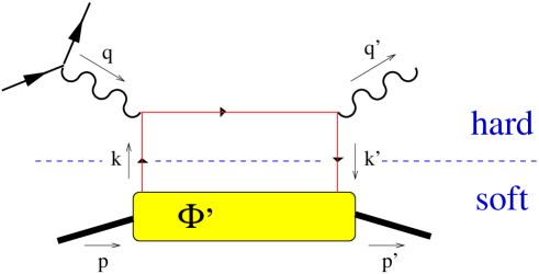
The notation for the momenta involved is indicated in Fig.1; the momentum transfer is denoted . We use light-cone components of four-vectors defined as for an arbitrary vector , and the argument of the second quark field is a shorthand for the point on the light-cone. The SPDs depend on the fractional momentum of the emitted quark , the ‘skewedness’ parameter which denotes the difference of momentum fractions on the two quark lines, and the invariant momentum transfer squared . The above definition has to be compared with the one for the (polarized) quark distribution function in a nucleon
| (2) |
In the forward case, i.e. for a matrix element diagonal in the nucleon momenta, there are no analogues of the helicity-flip terms and . In contrast, helicity-flip terms show up in the definition of the electromagnetic nucleon form factors
| (3) |
where initial and final nucleon momenta are different. The form factors , , , and are the Dirac, Pauli, the axial and the pseudoscalar form factors, respectively. By comparison reduction formulas can be read off as
where the formal forward limit implies . The lowest moments in , from which the dependence drops, relate the SPDs to form factors
3 CONNECTION TO LIGHT-CONE WAVE FUNCTIONS
Like the ordinary (forward) parton distributions also SPDs acquire a simple interpretation as probability densities in terms of quanta of ‘good’ components of the fields. The ‘good’ components of the quark fields are projected out as with and have a momentum decomposition
| (4) | |||||
where we use a collective notation for the dependence on the plus and transverse momentum components, and on the helicity in the form . The operators and are the annihilator of the plus component of the quark fields and the creator of the plus component of the antifields, respectively. They fulfill the equal light-cone time anticommutation relations [12]
| (5) |
The key point for a probabilistic interpretation is the observation that the quark field operator in the definition of the hadronic matrix elements is a density in terms of the ‘good’ components, i.e.
| (6) |
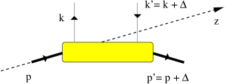
The quark SPD describes the emission of an (anti-)quark from the nucleon with a certain momentum fraction and its subsequent reabsorption with a different momentum fraction . In addition there is a kinematical region where the nucleon emits (or absorbs) a quark-antiquark pair. In fixing the notations for momenta and their fractions one has to define the longitudinal direction (i,.e. to chose a frame of reference). Two different popular choices are indicated in Fig.2 characterized by the momentum fractions (, ) and (, ), respectively. In this contribution we adhere throughout to the first choice and follow the notations in [7].

A connection between light-cone wave functions and form factors can be established by assuming that the nucleon states may be replaced by a superposition of partonic Fock states containing quanta of the ‘good’ light-cone components of (anti-)quark and gluon fields
| (7) |
with
| (8) |
and where is the light-cone momentum wave function of the parton Fock state. The index is a collective quantum number and labels the different ways of coupling the partons into the nucleon. Using the momentum decomposition of the quark field operators and the commutation relations for the creation and annihilation operators one derives the well-known Drell-Yan formula for the contribution of the parton Fock state to the Dirac form factor [13]
| (9) |
where the index denotes the active parton and runs over all partons of type with charge . The full form factor is obtained by summation over all Fock states. The shifted transverse momenta in the argument of the final state wave function are to be taken as for the spectator partons, and for the active quark. Note that the arguments of the wave functions are light-cone momentum fractions and transverse momenta of the partons with respect to their parent nucleon momenta, which are different for initial and final nucleon. The most convenient way to identify those arguments consists in performing transverse boosts to reference frames where the parent hadrons have no transverse momentum components. The shift in the transverse momenta of the spectator partons is the result of the appropriate transverse boosts, whereas the shift for the active quark combines the effects of absorbing the virtual photon and the one of the transverse boost.
The contribution of the parton Fock state to the ordinary quark parton distributions are straightforwardly obtained as
| (10) |
based on the probabilistic interpretation. Given the relations (9) and (10) and the close relationship between SPDs, forward distributions and form factors it is suggestive that there must be a similar way to obtain the SPDs from light-cone wave functions. Indeed, following along the same lines as in the derivation of the above formulas results in a generalization of the Drell-Yan formula valid in the partonic regimes, i.e. for and .
| (11) |
the index running over all quarks of flavor . The shifted arguments in the final state wave function are to be taken as
| (12) |
for the spectator partons and
| (13) |
for the active quark. Equation (11) was was obtained in [14] identifying the dominant contributions in a diagrammatic approach. In [14] and [15] the connection between SPDs and light-cone wave functions was exploited phenomenologically by explicitely modeling the wave function. Different inclusive and exclusive quantities like the electromagnetic form factors of proton and neutron, unpolarized and polarized forward parton distributions, and cross sections of wide angle real and virtual Compton scattering were studied in a consistent way. A detailed presentation of the derivation of an overlap formula for SPDs in the context of light-cone quantization, as briefly indicated in this contribution, will be given elsewhere [16].
References
- [1] F. M. Dittes, D. Muller, D. Robaschik, B. Geyer and J. Horejsi, Phys. Lett. B209, 325 (1988).
- [2] D. Muller, D. Robaschik, B. Geyer, F. M. Dittes and J. Horejsi, Fortsch. Phys. 42, 101 (1994) [hep-ph/9812448].
- [3] X. Ji, Phys. Rev. D55, 7114 (1997) [hep-ph/9609381].
- [4] X. Ji, J. Phys. G G24, 1181 (1998) [hep-ph/9807358].
- [5] A. V. Radyushkin, Phys. Lett. B380, 417 (1996) [hep-ph/9604317].
- [6] A. V. Radyushkin, Phys. Lett. B385, 333 (1996) [hep-ph/9605431].
- [7] A. V. Radyushkin, Phys. Rev. D56, 5524 (1997) [hep-ph/9704207].
- [8] J. C. Collins, L. Frankfurt and M. Strikman, Phys. Rev. D56, 2982 (1997) [hep-ph/9611433].
- [9] X. Ji and J. Osborne, Phys. Rev. D58, 094018 (1998) [hep-ph/9801260].
- [10] J. C. Collins and A. Freund, Phys. Rev. D59, 074009 (1999) [hep-ph/9801262].
- [11] X. Ji, Phys. Rev. Lett. 78, 610 (1997) [hep-ph/9603249].
- [12] S. J. Brodsky and G. P. Lepage, SLAC-PUB-4947 IN *MUELLER, A.H. (ED.): PERTURBATIVE QUANTUM CHROMODYNAMICS* 93-240 AND SLAC STANFORD - SLAC-PUB-4947 (89,REC.JUL.) 149p.
- [13] S. D. Drell and T. Yan, Phys. Rev. Lett. 24, 181 (1970).
- [14] M. Diehl, T. Feldmann, R. Jakob and P. Kroll, Eur. Phys. J. C8, 409 (1999) [hep-ph/9811253].
- [15] M. Diehl, T. Feldmann, R. Jakob and P. Kroll, Phys. Lett. B460, 204 (1999) [hep-ph/9903268].
- [16] M. Diehl, T. Feldmann, R. Jakob and P. Kroll, hep-ph/0009255.