SPECTATOR EFFECTS AND
QUARK-HADRON DUALITY IN
INCLUSIVE BEAUTY DECAYS

S. ARUNAGIRI, M.Sc.,
Department of Nuclear Physics

School of Physical Sciences

University of Madras

Guindy Campus

Chennai 600 025, INDIA

0.1 Preface

This Thesis is a review of the inclusive decays of heavy hadron. It is based on the author’s study of two issues which are important in the description of the inclusive beauty decays given by the heavy quark expansion.

• Evaluation of the expectation values of the four-quark operators in the heavy quark expansion,

• Study on the validity of the quark-hadron duality in the heavy quark expansion.

We evaluate the four-quark operators in two approaches: (1) in terms of the oscillator strength of the hadrons in the harmonic oscillator model, and (2) from the difference in the total decay rates of beauty hadrons under $SU(3)$ flavour symmetry. The results obtained indicate that the lifetime difference between $B$ meson and $\Lambda_{b}$ can be explained within heavy quark expansion by including the third order contribution.

To discuss the quark-hadron duality, the power corrections to the partonic decays rate are obtained in terms of the gluon mass which is assumed to imitate the short distance nonperturbative effects, by the choice $\lambda^{2}\gg\Lambda_{QCD}^{2}$.

The Thesis is organised in six Chapters, as follows:

• 1 Introduction: The Standard Model is briefly discussed and then the Spin-flavour symmetry exhibited by heavy hadrons is reviewed.

• 2 Four-quark operators: The author’s works on the evaluation of four-quark operators are presented.

• 3 Spectator effects: Presented are the calculation of ratio of lifetimes of beauty hadrons, particularly, $\tau(\Lambda_{b})/\tau(B)$ and the inclusive charmless semileptonic decay rate and determination of the CKM matrix element $|V_{ub}|$.

• 4 Short distance nonperturbative corrections: The renormalons contribution to the heavy quark expansion is discussed based on the authors work.

• 5 Quark-hadron duality: The validity of the assumption of quark-hadron duality is qualitatively discussed.

• 6 Conclusion: Conclusion of the Thesis with outlook of the works done are given.

  I am glad to acknowledge that my acquaintance with heavy quark physics began with the lectures on the heavy quark symmetry by Prof. Apoorva Patel during a discussion meeting at the Centre for Theoretical Studies, Indian Institute of Science, Bangalore. I got this great opportunity due to the invitation of Prof. J. Pasupathy. My learning of QCD is due to them by the way of their invitation to the discussion meetings conducted by them. I am grateful to both of them for their continuing support.

S. ARUNAGIRI

0.2 Acknowledgements

I thank Prof. P. R. Subramanian, Head of this Department, who has supervised my Thesis work and encouraged me to do things independently.

I am greatly indebted to Prof. H. S. Sarath Chandra, The Institute of Mathematical Sciences, Chennai, for discussions and kind attitude towards me. I place on record my deep gratitude to Prof. Hitoshi Yamamoto, University of Hawaii, USA, for a collaboration and sharing his wisdom. My sincere gratitude are due to Prof. Yasuhiro Okada, Theory Group, KEK, Japan, for extending me an invitation to KEK and useful discussions. I thank Prof. S. Narison, University of Montpellier, France, who clarified many doubts on renormalons.

I am grateful to Prof. M. Neubert, Cornell University for useful communications. My sincere thanks are due to Prof. M. Voloshin, University of Minnesota, USA for clarifications and discussions.

I enjoyed the comradeship with Dr. D. Caleb Chanthi Raj, SRM Engineering College, Chennai, Dr. J. Segar, RKM Vivekananda College, Chennai, and Dr. R. Premanand, SRM Engineering College, Chennai. With their helps and affection only, I derived strength to bear joys and sorrows during this programme.

I acknowledge the interests shown on me and my works by Prof. V. Devanathan and Prof. T. Nagarajan, former heads of this Department, the faculty members and other staff of the Department of Nuclear Physics.

It is a pleasure for me to be with Prof. K. Raja, Dr. N. Baskaran, Dr. Manivel Raja, Dr. R. N. Viswanath, Dr. R. Ramamoorthy, Messers A. Chandra Bose, N. Ponpandian, R. Justin Joseyphus, K. Ravichandran, R. Shanmugam, B. Nagarajan, B. Soundarajan and R. Sudharsan. I thank them for their help.

I thank the authorities of The Institute of Mathematical Sciences for allowing me to use their library and computing facilities.

I am grateful to Mr. V. Swaminathan who has been pouring passionate interest in me and my scheme of things and Mr. C. Krishnamoorthy for his helps.

I express my deep sense of gratitude to (Late) Mr M. Arangarajan who had inspired me as a brother, a mentor and a friend from my childhood and his family members. I appreciate the forbearance of my father Mr R. Somasundaram and the other members of our family who stood by me in successful completion of this programme.

S. ARUNAGIRI

0.3 List of Publications

1. Colour-straight four-quark operators and lifetimes of b-flavoured hadrons,
   S. Arunagiri, Int. J. Mod. Phys. A 15 (2000) 3053 - 3063 [hep-ph/9903293]

2. A note on spectator effects and quark-hadron duality in inclusive beauty decays
   S. Arunagiri, Phys. Lett. B 489 (2000) 309-312 [hep-ph/0002295].

3. Inclusive charmless semileptonic decay of $\Lambda_{b}$ and $Br(b\rightarrow X_{u}l\nu)$
   S. Arunagiri and H. Yamamoto [hep-ph/0005266].

4. On the short distance nonperturbative corrections in heavy quark expansion
   S. Arunagiri, presented in the XVIII International Symposium on Lattice Field Theory, held at Bangalore, India, during August 17-22, 2000 [hep-ph/0009109].

5. Spectator effects in inclusive beauty decays
   Contributed to the Working group report on B and collider physics, Proc. VI Workshop on High Energy Physics Phenomenology, held at Chennai, India, during January 3-15, 2000,
   Pramana - J. Phys. 55 (2000) 335-345 [hep-ph/0004002].

6. Pattern of lifetimes of beauty hadrons and quark-hadron duality in heavy quark expansion
   S. Arunagiri, to be published in the Proceedings of IV Workshop on Continuos Advances in QCD, held at Minneapolis, USA, during May 12 - 14, 2000 [hep-ph/0009110].

Chapter 1 Introduction

This Chapter consists of two sections: The first is devoted to the Standard Model and in the second the heavy quark symmetry and the heavy quark expansion are discussed .

1.1 Standard model

In this section, we briefly describe the texture of the Standard Model and remark on the perspectives of the weak decays of heavy hadrons in the Standard Model.

1.1.1 Quarks, Leptons, and Hadrons

Today, our knowledge is, as embodied in the Standard Model, firm about the primitive constituents of matter [1]. They are six quarks and six leptons, all fermions. The quarks are interacting through all the known three interactions of the elementary particles in nature: electromagnetic, weak and strong, but the leptons do not strongly interact. Both of them are not influenced by the gravity effects. The interactions are mediated by (gauge) bosons: photon, $W^{\pm},Z^{0}$ and gluon. The properties of these fermions and bosons are given in Tables 1.1 and 1.2 [2].

The fermions make up the hadrons: meson, a bosonic hadron, of a quark-antiquark pair and baryon, a fermionic hadron, of three quarks. Quark structure of hadrons is described, for three quarks $u,d$ and $s$, under $SU(3)$ flavour symmetry by the Gell-Mann - Nishijima relation:

$$Q=I_{z}+(B+S)/2$$ (1.1)

where $Q$ is the electric charge of the hadron, in units of $e$, $I_{z}$ the third component of the isospin, $B$ the baryon number, and $S$ the strangeness quantum number. Each quark is assigned a colour quantum number. Each quark carries three colours but the quarks make hadrons colour singlet. For mesons, $B=0$. This can be extended to the charm and beauty quarks as well. The situation is different in the case of top which decays before hadronising. The rate of top quark weak decay, $\Gamma(t\rightarrow bW)$ [3], is found to be larger than the QCD scale that corresponds to the typical hadron size.

Table 1.1: Quarks and Leptons (^a in GeV/c²; ^b in $e$ units; ^c quantum numbers; ^d charge of leptons except neutrinos is $-1$)

Quark	Massa	Chargeb	Qu. nos.c	Leptond	Mass
up, $u$	(1.5 - 5) $.10^{-3}$	$+{2\over 3}$	$I_{z}=+{1\over 2}$	$e^{-}$	0.51 $.10^{-3}$
down, $d$	(3 - 9) $.10^{-3}$	$-{1\over 3}$	$I_{z}=-{1\over 2}$	$\mu^{-}$	0.105
strange, $s$	0.060 - 0.170	$-{1\over 3}$	$s=-1$	$\tau^{-}$	1.777
charm, $c$	1.1 - 1.4	$+{2\over 3}$	$c=1$	$\nu_{e}$	10-15 $.10^{-6}$
bottom, $b$	4.1 - 4.4	$-{1\over 3}$	$b=-1$	$\nu_{\mu}$	$<0.17.10^{-3}$
top, $t$	170	$+{2\over 3}$	$t=1$	$\nu_{\tau}$	$<18.10^{-3}$

Table 1.2: Force carriers

Gauge Boson	Mass	Charge	Force	Strength
photon, $\gamma$	0	0	electromagnetic	1/137
$W$	80	$\pm$ 1	weak	1.1663692 GeV-2
$Z$	90	0	weak
gluon, $g$	0	0	strong	0.12 at $M_{Z}$

In the next section we present a brief review of the Standard Model (SM). The SM is a renormalisable field theory of the local gauge group $SU(3)_{C}\times SU(2)_{L}\times U(1)_{Y}$ [4]. It is a unified theory of strong ($SU(3)_{C}$), weak ($SU(2)_{L}$) and electromagnetic ($U(1)_{Y}$) interactions at $TeV$ scale. The SM contains two sectors: quantum chromodynamics and electroweak [5].

1.1.2 Quantum Chromodynamics

A prelude

In the proposal of quark structure of hadrons made by Gell-Mann and Zweig, the quarks are described in terms of flavour and colour as required to explain the known properties of hadrons. The idea of quarks carrying colour got confirmed by the measured normalisation of the decay rate $\Gamma(\pi^{0}\rightarrow 2\gamma)$ and the cross-section $\sigma(e^{+}e^{-}\rightarrow hadrons)$. Using current algebra, the strong interaction between quarks is shown to be mediated by massless vector bosons, gluons, analogous to photon of electromagnetic interaction. According to the colour assignment to quarks, gluons form an octet.

Lepton ($e^{-}/\nu$) - proton deep inelastic scattering experiments confirmed the composite structure of a proton. Further, from the deep inelastic scattering experiments, it was found that quarks and gluons are freely roaming around inside the proton. This behaviour is explained by Bjorken through his scaling law that at small distance (this corresponds to large momentum transferred), the quarks are behaving as if they are free, but at large distance (i. e., small momentum transferred), they are confined in pair. The former property is known as asymptotic freedom and the latter confinement.

The Lagrangian of QCD

Theory of quarks and gluons is based on the local non-abelian gauge group $SU(3)_{C}$ symmetry[6]. With the work of ’t Hooft on renormalisability of Yang-Mills theories [7], the theory of strong interaction is formulated. The basic Lagrangian is

$${\cal L}_{QCD}=-{1\over 4}F^{a}_{\mu\nu}F_{a}^{\mu\nu}+\sum_{f}\bar{q}^{f,a}(x)i\gamma_{\mu}D^{\mu}q(x)^{f}_{b}-\sum_{f}m_{f}\bar{q}^{f,a}(x)q(x)^{f}_{b}$$ (1.2)

where the indices $a,b$ stand for colour and $f$ for flavour of quarks and

$$F_{\mu\nu}^{a} = \partial_{\mu}A_{\nu}^{a}-\partial_{\nu}A_{\mu}^{a}-g_{s}f^{abc}A_{\mu}^{b}A_{\nu}^{c},\hskip 14.22636pt$$ (1.3)

$$D_{\mu}^{a} = \partial_{\mu}^{a}+ig_{s}t^{a}A_{\mu}^{a}$$ (1.4)

where $g_{s}$ is the strong coupling constant, $f^{abc}$ the structure constant of $SU(3)$ Lie algebra and $t^{a}={1\over 2}\lambda^{a}$, with $\lambda^{a}$ being the Gell-Mann colour $(3\times 3)$ matrices. In Eq. (1.2), the first term is the gluon part, the second the quarks part and the quark-gluon interaction part and the third the quark mass contribution. The Lagrangian is invariant under the local gauge group $SU(3)$. The gauge transformation is given by $U(x)=e^{it^{a}\xi^{a}(x)}$ where $\xi^{a}(x)$ is an infinitesimal gauge parameter with $a$ running from 1 to 8. The $t^{a}$ are the generators of the gauge group. Because of the non-Abelian nature of the boson field, gluons can be described as self-interacting, vector bosons. The Lagrangian, in (1.2), is supplemented by additional terms corresponding to gauge-fixing, ghost and counter terms for perturbative treatment. With these terms, one can get the Feynman rules for QCD.

The QCD Lagrangian, in the limit of $m_{q}=0$, where $q=u,d,s$, is invariant under the chiral symmetry group $SU(3)_{L}\times SU(3)_{R}$ [8]. On the other extreme, for quarks of mass $m_{Q}\gg\Lambda_{QCD}$, in the limit $m_{Q}\rightarrow\infty$, the Lagrangian exhibits spin-flavour symmetry [9] which will be discussed in details in the next chapter. Besides , ${\cal L}_{QCD}$ possesses stability against weak radiative corrections due to the flavour-neutrality of the gluon.

Perturbative QCD: Running Coupling and Running Mass

Different renormalisation schemes are used to make the Lagrangian free of divergences. Then the renormalised quantities are defined at some chosen scale [10]. Different choice of the scale leads to different physical values for the same quantity. In order to circumvent the scale dependence, renormalisation group equations are used. The scale transformation, $\mu\rightarrow\mu^{\prime}$, constitutes a renormalisation group. Under this group, the physical quantities, explicitly or implicitly scale dependent, are invariant. Such a study is due to Callan-Symansik. In the $MS$ or $\overline{MS}$ scheme, for the coupling constant, the Callan-Symasik or renormalisation group equation is given by

$$d\bar{g}(\mu)/d\log\mu=\bar{g}(\mu)\beta(\bar{g}(\mu))$$ (1.5)

An expansion of $\beta$ in $\bar{g}(\mu)$ yields, at the lowest order,

$$\beta=-\beta_{0}{\bar{g}(\mu)^{2}\over{16\pi^{2}}},\hskip 14.22636pt\beta_{0}={11C_{A}\over 3}-{4n_{f}T_{F}\over 3}$$ (1.6)

where $C_{A}=3,T_{F}=1/2$ and $n_{f}$ is the number of flavours. Now, defining the running coupling constant $\alpha_{s}=\bar{g}^{2}/4\pi$, with $\mu=Q^{2}/\nu^{2}$,

$$\alpha(Q^{2})={4\pi\over{\beta_{0}\log\left({Q^{2}/{\Lambda^{2}}}\right)}},$$ (1.7)

$$\Lambda^{2}=\nu^{2}e^{-{4\pi/{\alpha(\nu^{2})}}}$$ (1.8)

where $\Lambda_{QCD}$ is known as the QCD scale parameter, which is the constant of integration. From (1.8), it is obvious that as $Q^{2}\rightarrow\infty,\alpha_{s}\rightarrow 0$. This behaviour is the celebrated asymptotic freedom [11]. For finite but sufficiently large $Q^{2}$, $\alpha_{s}$ is employable as a perturbation parameter.

Similarly, the running mass $\bar{m}(Q^{2})$ is given by

$$\bar{m}(Q^{2})=m_{0}\left[{1\over 2}\log\left({Q^{2}\over{\Lambda^{2}}}\right)\right]^{-d_{m}}$$ (1.9)

where $m_{0}$ is the invariant mass and $d_{m}$ is known as the anomalous mass dimension, given by $4/\beta_{0}$.

A digression

The perturbation series of a physical quantity in terms of $\alpha_{s}$ is known to few orders. A quantity is said to be defined completely, if the expansion in $\alpha_{s}$ is made to all orders. But it is impossible to define them to $n$ orders, where $n$ is large. At large order, as first discovered in QED by Dyson in 1952, the series in $\alpha_{s}$ factorially diverges. This issue has attracted interests recently after it was first pointed out by ’t Hooft in 1977 that the inherent ambiguities in the perturbative definition of a quantity is $O\left({\Lambda_{QCD}/Q}\right)$ and beyond. These ambiguities are known as renormalons [12]. These corrections are seen to be important as they would represent the first nonperturbative corrections to the leading order of the OPE.

The QCD needs to be dealt with at small and large distance scales separately. Any physical amplitude of a QCD process described by the product of operators can be separated into two parts by the Wilson short distance or operator product expansion [13]. As a result, the short distance physics is contained in the expansion coefficients, which happen to be $c$-numbers, and the local operators describe the long distance aspect. While the perturbative QCD successfully describes the short distance processes, the long distance aspects being nonperturbative are poorly understood. However, there are semi analytic methods such as QCD or SVZ sum rules [14] and lattice gauge theory [15].

1.1.3 Electroweak Theory

Fermi theory of weak interaction

With the explanation of the the radioactive decay of a nucleus, the weak force was discovered. For example, weak interaction drives a neutron to change into a proton with a lepton pair, electron and its antineutrino, inside the nucleus. At the quark level, it is the transition of the $d$ quark into the $u$ quark plus a lepton pair. A theoretical description of weak interaction emerged due to Yang and Lee, and Wu et al [16] following Fermi. The Lagrangian of weak interaction is then given by

$${\cal L}_{Fermi}={G_{f}\over{\sqrt{2}}}J^{\mu}(x)J_{\mu}^{{\dagger}}(x)+h.c.,$$ (1.10)

where $G_{f}=1.16637\pm 0.00001GeV^{-2}$ is the Fermi coupling constant and the weak current $J^{\mu}$ is given by

$$J^{\mu}(x)=\bar{p}(x)\gamma^{\mu}(g_{V}-g_{A}\gamma_{5})n(x)\bar{e}^{-}(x)\gamma_{\mu}(1-\gamma_{5})\nu_{e^{-}}(x),$$ (1.11)

where the vector coupling $g_{V}$ is little less than one and is given in terms of the Cabibbo angle to be 0.97. The ratio of the coupling constants $g_{A}/g_{V}=-1.2573\pm 0.0028$ [2].

Towards formulating a complete theory of weak interaction, it is postulated that the weak interaction is mediated by a vector boson, massive due to weak interaction being point-like. The additional requirements of such a boson are that it has to be charged both positively and negatively because of charge-changing weak current and having indefinite parity to preserve the $V-A$ structure of the weak current. Thus, the Lagrangian is

$${\cal L}_{W}=-g_{W}J^{\mu}(x)W_{\mu}(x)+h.c.$$ (1.12)

where $W(x)$ is the vector boson field and $g_{W}$ the dimensionless weak coupling constant which is related to the Fermi coupling constant by

$${g_{W}^{2}\over{8M_{W}^{2}}}={G_{f}\over\sqrt{2}}$$ (1.13)

The Lagrangian in (1.12) is useful at low energy but not renormalisable. The existence of $W^{\pm}$ is another way of looking at $G_{F}$. The step towards the renormalisable theory of weak interaction results in the unification of the weak and the electromagnetic interactions, electroweak interaction.

An interlude

The current-current interaction described by (1.12) is applicable only for charged current. There is also a neutral current mediated weak interaction. If both are combined, then three massive vector bosons correspond to the isospin triplet of weak currents. This obviously leads to $SU(2)_{L}$ symmetry of weak interaction. The fermion field is a left handed doublet. Then, the current is of the form

$$J_{\mu}^{i}(x)=(\bar{\nu}\hskip 9.95863pt\bar{e})_{L}\gamma_{\mu}{\tau_{i}\over 2}\left(\begin{array}[]{l}\nu\\ e^{-}\end{array}\right)_{L}$$ (1.14)

where $\tau_{i}$ is the isospin triplet. Since the weak neutral current, $J_{\mu}^{NC}$, has a right handed component, the neutral component of (1.14) is not a weak current. However, this can be identified with the electromagnetic current

$$j_{\mu}=ej_{\mu}^{em}=e\bar{\Psi}\gamma_{\mu}Q\Psi$$ (1.15)

where $Q$ is the charge operator with eigenvalue –1 for electron and the generator of $U(1)$ symmetry. Under orthogonal combination

$$j_{\mu}^{em}=J_{\mu}^{3}+{1\over 2}J_{\mu}^{Y}$$ (1.16)

The consequence of the above equation is the relation, $Q=T^{3}_{W}+Y_{W}/2$, weak counterpart of (1.1), where $T^{3}_{W}$ is the weak isospin and $Y_{W}$ the weak hypercharge. Like $Q$, $Y_{W}$ generates the $U(1)_{Y}$ symmetry group. Thus, this yields the $SU(2)_{L}\times U(1)_{Y}$ gauge group. The fundamental fermions, quarks and leptons, come in three generations or families with weak isospin and weak hypercharge quantum numbers as shown in the Table 1.3.

Table 1.3: Assignment of quantum numbers in $SU(3)_{L}\times U(1)_{Y}$

generation	$T_{L}^{3}$	$Y_{L}$	$T_{R}^{3}$	$Y_{R}$
u     c     t	1/2	1/6	0	2/3
d     s     b	-1/2	1/6	0	-1/3
$\nu_{e}\hskip 8.5359pt$ $\nu_{\mu}\hskip 8.5359pt$ $\nu_{\tau}$	1/2	-1/2	0	0
$e\hskip 8.5359pt$ $\mu\hskip 8.5359pt$ $\tau$	-1/2	-1/2	0	-1

Electroweak Lagrangian

The electroweak Lagrangian of the non-Abelian local gauge $SU(2)_{L}\times U(1)_{Y}$ symmetry is of the form

$${\cal L}_{ew} = -{1\over 4}W^{i,~{}\mu\nu}W^{i}_{\mu\nu}-{1\over 4}B^{\mu\nu}B_{\mu\nu}+2\sum_{f=1}^{3}\bar{\Psi}^{f}_{L}\gamma_{\mu}D^{\mu}\Psi^{f}_{L}$$ (1.17)

$$D^{\mu} = \partial^{\mu}+igt^{i}W^{i,\mu}+ig^{\prime}YB^{\mu}$$ (1.18)

where $g$ and $g^{\prime}$ are coupling constants. We get the photon field and the $Z^{0}$ field as the linear combination of $W^{3}$ and $B$ coupled to the electromagnetic current:

$$A_{\mu} = -\sin\theta_{W}W^{3}_{\mu}+\cos\theta_{W}B_{\mu},$$ (1.19)

$$Z_{\mu} = \cos\theta_{W}W^{3}_{\mu}+\sin\theta_{W}B_{\mu}$$ (1.20)

where $\tan\theta_{W}={g^{\prime}/g},\hskip 4.26773pte=g\sin\theta_{W}$ The interaction part is

$${\cal L}_{I}=-\left\{{g\over{2\sqrt{2}}}J_{\mu}^{+}W^{-,\mu}+{g\over{2\sqrt{2}}}J_{\mu}^{-}W^{+,\mu}\\ +eJ_{\mu}^{em}A^{\mu}\right\}$$ (1.21)

The currents are given by

$$J_{\mu}^{+} = \sum\bar{q}\gamma_{\mu}(1-\gamma_{5})V_{CKM}q+\sum\bar{l}\gamma_{\mu}(1-\gamma_{5})l$$ (1.22)

$$J_{\mu}^{NC} = \sum\bar{\Psi}\gamma_{\mu}(v-a\gamma_{5})\Psi$$ (1.23)

$$J_{\mu}^{em} = \sum\bar{\Psi}\gamma_{\mu}Q\Psi$$ (1.24)

where $V_{CKM}$ is the CKM matrix of flavour mixing (see below) and $v=T^{3}_{L}-2Q\sin^{2}\theta_{w},a=T^{3}_{L}$.

Spontaneous breaking of symmetry

In the electroweak Lagrangian in (1.18), introducing a mass term for both fermions and gauge bosons is forbidden by gauge invariance. However, the Higgs mechanism of spontaneous breaking of the $SU(2)_{L}\times U(1)_{Y}$ symmetry [17] gives mass for the fermions and the three bosons of weak interaction. For the Higgs doublet field, $\Phi$,

$$\Phi=\left(\begin{array}[]{l}\phi^{+}\\ \phi^{0}\end{array}\right)$$ (1.25)

the Lagrangian is of the form

$${\cal L}_{\phi}(x) = (D^{\mu}\Phi)^{{\dagger}}(D_{\mu}\Phi)-\sum_{\chi}f_{\chi}\bar{\chi}_{L}\tilde{\Phi}\chi_{R}+\mu^{2}\Phi^{*}\Phi-\lambda(\Phi^{{\dagger}}\Phi)^{2}$$ (1.26)

$$D_{\mu}\Phi = ({\bf I}(\partial_{\mu}+i{g\over 2}B_{\mu})+ig^{\prime}{\tau_{i}\over 2}W_{\mu})\Phi$$ (1.27)

In (1.26), the three terms stand for free, Higgs-fermion interaction and potential parts as in the order given. Minimising the potential, ground state Higgs field is

$$\Phi=\left(\begin{array}[]{l}0\\ v/\sqrt{2}\end{array}\right),\hskip 14.22636ptv=\sqrt{{\mu^{2}\over\lambda}}$$ (1.28)

This non-vanishing field describes the spontaneous breaking of the electroweak symmetry. Thus, the masses of fermions and bosons are generated:

$${\cal L}_{mass}= - {v\over{\sqrt{2}}}\sum f_{a}\bar{a}a+\left({vg^{\prime}\over 2}\right)^{2}W_{\mu}^{+}W^{-,\mu}$$ (1.33)

$$+ {v^{2}\over 8}(W_{\mu}^{3}\hskip 9.95863ptB_{\mu})\left(\begin{array}[]{ll}{g^{\prime}}^{2}&-gg^{\prime}\\ -gg^{\prime}&g^{2}\end{array}\right)\left(\begin{array}[]{l}W^{3,\mu}\\ B^{\mu}\end{array}\right)$$

where $a$ stands for all the fermions, excluding the neutrinos.

Masses for the bosons and the fermions (but not neutrinos) are, then, given by

$$m_{a} = {v\over\sqrt{2}}f_{a},\hskip 28.45274pta=u,d,e,...$$ (1.34)

$$M_{W} = {v\over 2}g^{\prime},\hskip 34.14322ptM_{Z}={v\over 2}\sqrt{g^{2}+{g^{\prime}}^{2}}$$ (1.35)

$$M_{\gamma} = 0$$ (1.36)

Quarks mixing

Mixing of different flavours is caused by the charged current mediated by $W^{\pm}$. The quark-mixing matrix, $V_{CKM}$, in (1.22) is a unitary (3 $\times$ 3) matrix [18].

$$V_{CKM}=\left(\begin{array}[]{lll}V_{ud}&V_{us}&V_{ub}\\ V_{cd}&V_{cs}&V_{cb}\\ V_{td}&V_{ts}&V_{tb}\end{array}\right)$$ (1.37)

By the above equation, the weak basis, $q^{\prime}$ and mass basis $q$ are related by $\bar{q}_{i}^{\prime}=V_{ij}q_{j}$ The unitarity of the matrix $V$ is: $V_{ij}\rightarrow exp(i\phi_{i})V_{ij}exp(-i\phi_{j})$.

Further, the elements of the CKM matrix satisfy unitarity constraints: any pair of rows or columns are orthogonal. There are six constraints (1.37). For example,

$$V_{ud}V_{td}^{*}+V_{us}V_{ts}^{*}+V_{ub}V_{tb}^{*}=0$$ (1.38)

This is useful to determine one element from the others.

1.1.4 Weak Decays of Heavy Hadrons

Knowledge of the weak decays of beauty hadrons, especially $B$ mesons, is an important requirement to test the Standard Model [19]. Of about twenty input parameters, nine are the CKM matrix elements. The unitarity test of the CKM matrix demands precise prediction of its elements. The determination of $V_{ub},V_{cb},V_{tb},V_{ts}$, and $V_{td}$, involves the $b$ hadron weak processes: the charged current mediated modes, viz., the dominant $b\rightarrow c+Y$, and the CKM suppressed, $b\rightarrow u+Y$ determine $V_{cb}$ and $V_{ub}$ respectively; the rare decays of the neutral current, $b\rightarrow s+Y$ and $b\rightarrow d+Y$ respectively determine $V_{ts}$ and $V_{td}$; and the weak decay, mediated by the charged current, $t\rightarrow bW$, determines $V_{tb}$. ($Y$ denotes either a lepton pair or a quark pair or a photon/gluon.). Precise determination of the elements of the CKM matrix is stringent need for checking the CKM model of the CP violation in the SM [20].

The heavy hadrons, hadrons containing a heavy quark whose mass $m_{Q}\gg\Lambda_{QCD}$, is easier to study from the QCD point of view. For, the coupling constant is smaller at $m_{Q}$ and the Compton wavelength of the heavy quark, $1/m_{Q}$, is much smaller than $\Lambda_{QCD}^{-1}$. Thus, a lot of simplification arises in describing the properties and decays of these hadrons. In the limit, $m_{Q}\rightarrow\infty$, with the resultant so called heavy quark symmetry, we get a low energy description of these heavy hadrons. This enables a model independent prediction of the CKM matrix elements $|V_{ub}|$ and $|V_{cb}|$.

1.2 Hadrons with Spin-flavour Symmetry

In this section, we discuss the spin-flavour symmetry or heavy quark symmetry exhibited by the hadrons containing a heavy quark, quark of mass $m_{Q}\gg\Lambda_{QCD}$. Then, we describe the theory of inclusive decays of heavy hadrons[9, 21, 22, 23].

1.2.1 Spin-flavour symmetry

Because the heavy quark mass can be taken to the asymptotic limit, the study of weak interaction of the heavy hadrons becomes simplified [24, 25, 26, 27]:

• the asymptotic freedom: the coupling constant is small enough to allow perturbative calculations;

• the Compton wavelength of the heavy quark, $1/m_{Q}$, is much greater than the typical hadron size, $1/\Lambda_{QCD}$.

In the limit $m_{Q}\rightarrow\infty$, the heavy quark acts as a static source of colour inside the hadron. Since the light degrees of freedom cannot resolve the distances smaller that the typical hadron size, the light stuff interaction with the heavy quark vanishes. Consequently, either state of the heavy quark spin is independent of the other. Thus heavy quark spin generates the $SU(2)$ spin symmetry. On the other hand, the replacement of an infinitely heavy quark by another infinitely heavy quark does not change the description of the system. This leads to the flavour symmetry. Hence, for $N_{f}$ heavy flavours, the hadron concerned is described by $SU(2N_{f})$ symmetry, called spin-flavour or heavy quark symmetry.

In the static limit of the heavy quark, the four-velocity of the heavy quark is $v_{\mu}=(1,{\bf 0})$, i. e., the heavy quark is in the rest frame of the hadron containing it. Thus, both the decaying hadron and the corresponding final state are looking the same in this limit, since the product of the four-velocities of the initial and final state heavy quarks is unity.

Also the third components of the heavy quark spin, $\pm 1/2$ and that of the light quark(s), $j$ are separately conserved, $J=j\pm 1/2$. With the heavy quark symmetry, the heavy hadrons can be classified by the quantum numbers of the light degrees of freedom, viz., flavour, spin, parity, etc., but independent of heavy quark spin and mass [28]. As will be described in more detail later, the mass of the hadron is given by an expansion in the inverse powers of the heavy quark mass:

$$M_{H}=m_{Q}+\bar{\Lambda}+O(1/m_{Q})$$ (1.39)

where $\bar{\Lambda}$ stands for the energy of the light degrees of freedom. The term $O(1/m_{Q})$ is due to the kinetic energy of the heavy quark inside the hadron and the hyperfine mass splitting due to the spin orientation of the heavy quark with the light degrees of freedom. Its magnitude depends on the heavy quark mass, of the order of $\Lambda_{QCD}$.

Under the breakdown of the $SU(3)$ flavour symmetry, the $c$ and $b$ meson mass differences are of approximately same magnitude:

$$m_{B_{s}}-m_{B_{d}}=\bar{\Lambda}_{s}-\bar{\Lambda}_{d}$$ (1.40)

$$m_{D_{s}}-m_{D_{d}}=\bar{\Lambda}_{s}-\bar{\Lambda}_{d}$$ (1.41)

where the mass differences are respectively given by $90\pm 3$ and $99\pm 1$ MeV. Similarly, the mass difference between the baryon and the meson is given by:

$$m_{\Lambda_{b}}-m_{B}=\bar{\Lambda}_{\Lambda_{b}}-\bar{\Lambda}_{B}$$ (1.42)

$$m_{\Lambda_{c}}-m_{D}=\bar{\Lambda}_{\Lambda_{c}}-\bar{\Lambda}_{D}$$ (1.43)

Their values are predicted to be $346\pm 6$ and $416\pm 1$ MeV respectively. These mass differences receive corrections of $O(\Lambda_{QCD}/m_{Q})$.

1.2.2 Effective Theory

In the limit, $m_{Q}\rightarrow\infty$, the QCD Lagrangian turns out to be a low energy effective one as the heavy particle is irrelevant at low energies [29, 30, 31, 32, 33, 34, 35]. Now the theory is similar to the Fermi theory of weak interaction discussed in the previous section.

As mentioned earlier, in the heavy quark limit, the heavy quark is in the rest frame of the parent hadron and it is almost on-shell. Its momentum is

$$p_{Q}^{\mu}=m_{Q}v^{\mu}+k^{\mu}$$ (1.44)

where $k$ is the residual momentum of $O(\Lambda_{QCD})$. Accordingly, we define the propagator and the vertex function as

$${i\over{p_{Q}^{\mu}-m_{Q}}}={i\over{v.k}}{1+{\not\!v}\over 2}\hskip 8.5359pt~{}\mbox{and}\hskip 8.5359ptig_{s}v^{\alpha}T_{a}$$ (1.45)

respectively. In the above equation, $(1\pm{\not\!v})/2$ are the positive and negative projection operators. They act finitely on the large and small components of the fields respectively:

$$h_{v}(x)=e^{im_{Q}v.x}P_{+}Q(x),\hskip 25.6073ptH_{v}(x)=e^{-im_{Q}v.x}P_{-}Q(x)$$ (1.46)

such that

$$Q(x)=e^{-im_{Q}v.x}[h_{v}(x)+H_{v}(x)]$$ (1.47)

Because of the projection operator, the field defined above satisfies ${\not\!}vh_{v}=h_{v}$ and ${\not!v}H_{v}=-H_{v}$, where $h_{v}$ annihilates a quark of velocity $v$ and $H_{v}$ creates an heavy antiquark.

With these new fields, the QCD Lagrangian

$${\cal L}_{QCD}=\bar{Q}(x)(\not\!D-m_{Q})Q(x)$$ (1.48)

turns out to be of the following form for a heavy quark

$${\cal L}_{Q}=\bar{h}_{v}iv.Dh_{v}-\bar{H}_{v}(iv.D+2m_{Q})H_{v}+\bar{h}_{v}(i\not\!D_{\perp})H_{v}+\bar{H}(i\not\!D_{\perp})h_{v}$$ (1.49)

where $D^{\mu}_{\perp}=D^{\mu}-v^{\mu}$, $v.D$ satisfying $v.D_{\perp}$ = 0 in the rest frame, the $h_{v}$ term corresponds to the massless degrees of freedom and the $H_{v}$ term to the heavy degrees of freedom which have to be integrated out, with fluctuation being twice the heavy quark mass. By using the equation of motion, the heavy degrees of freedom, $H_{v}$, can be eliminated. That is by taking derivative of the above equation with respect to $\bar{H}_{v}$, we get the differential equation and its solution as

$$(iv.D+2m_{Q})H_{v}=i\not\!D_{\perp}h_{v},\hskip 14.22636ptH_{v}={1\over{2m_{Q}+iv.D}}i\not\!D_{\perp}h_{v}$$ (1.50)

Thus the nonlocal effective action results in

$${\cal L}_{eff}=\bar{h}_{v}iv.Dh_{v}+\bar{h}_{v}i\not\!D_{\perp}{1\over{2m_{Q}+iv.D}}i\not\!D_{\perp}h_{v}$$ (1.51)

where the second term corresponds to virtual processes. This Lagrangian can be expanded in powers of $1/m_{Q}$:

$${\cal L}_{eff}=\bar{h}_{v}iv.Dh_{v}+{1\over{2m_{Q}}}\sum_{n=0}^{\infty}\bar{h}_{v}i\not\!D_{\perp}\left({-iv.D\over{2m_{Q}}}\right)i\not\!D_{\perp}h_{v}$$ (1.52)

The Lagrangian is explicitly given as

$${\cal L}_{eff}=\bar{h}_{v}iv.Dh_{v}+{1\over{2m_{Q}}}\bar{h}_{v}(iD_{\perp})^{2}h_{v}+{g_{s}\over{4m_{Q}}}\bar{h}_{v}\sigma_{\mu\nu}G^{\mu\nu}h_{v}+O(1/m_{Q}^{2})$$ (1.53)

Thus, in the limit $m_{Q}\rightarrow\infty$, only the first term survives, which is independendent of the heavy quark mass:

$${\cal L}_{HQET}=\bar{h}_{v}iv.Dh_{v}$$ (1.54)

For this Lagrangian, the Feynman rules are given already in (1.45). In the above, we have applied the heavy quark limit to the effective Lagrangian, not the QCD Lagrangian. Thus, the heavy quark symmetry is not the symmetry of QCD but that of the low energy effective theory, (1.54). The corrections appear to ${\cal L}_{HQET}$ due to the finite mass of the heavy quark. As the heavy quark mass increases, the expansion becomes more and more powerful.

In the rest frame, the $O(1/m_{Q})$ operators are kinetic and chromomagnetic operators.

$$O_{kin}={1\over{2m_{Q}}}\bar{h}_{v}(iD_{\perp})^{2}h_{v}\rightarrow-{1\over{2m_{Q}}}\bar{h}_{v}(i\vec{D})^{2}h_{v}$$ (1.55)

which is the gauge covariant extension of the kinetic energy due to heavy quark motion.

$$O_{mag}={g_{s}\over{4m_{Q}}}\bar{h}_{v}\sigma_{\mu\nu}G^{\mu\nu}h_{v}\rightarrow-{g_{s}\over{m_{Q}}}\bar{h}_{b}\vec{S}\vec{B_{c}}h_{v}$$ (1.56)

is the non-Abelian analogue of the Pauli interaction describing the colour magnetic coupling of the heavy quark spin to the gluon field. In the above equation for the magnetic operator, the spin operator $\vec{S}$ and the component of the colour magnetic field $B^{i}_{c}$ are given by

$$S^{i} = {1\over 2}\left(\begin{array}[]{ll}\sigma^{i}&0\\ 0&\sigma^{i}\end{array}\right),\hskip 14.22636pt[S^{i},S^{j}]=i\epsilon^{ijk}S^{k}$$ (1.59)

$$B_{c}^{i} = -{1\over 2}\epsilon^{ijk}G^{jk}$$ (1.60)

The corrections appearing at the next-to-leading order and beyond can be expressed as the short and long distance parts entangled. While the short distance physics is contained in the Wilson coefficients, the long distance physics are given by the local operators.

As we have mentioned earlier (1.39), the energy of the light degrees of freedom $\bar{\Lambda}$ varies with the heavy quark mass. But the choice of the heavy quark mass is not unique. The mass previously referred to in this section is the mass in the Lagrangian. If one chooses it to be the pole mass, $m_{Q}$, then $\bar{\Lambda}$ is given in the asymptotic limit of the heavy quark mass as

$$\bar{\Lambda}=(M_{H}-m_{Q})|_{m_{Q}\rightarrow\infty}$$ (1.61)

If we define the heavy quark mass in some other scheme and at a certain scale, then $\bar{\Lambda}$ changes accordingly. However, if defined alternately as

$$\bar{\Lambda}-\delta m=(M_{H}-\bar{m}_{Q})$$ (1.62)

then the quantity $\bar{\Lambda}-\delta m$ is invariant, where $\delta m$ is known as the residual mass of the order of $\Lambda_{QCD}$ [36]. In that case, since the HQET allows the residual mass in the leading Lagrangian, ${\cal L}_{HQET}$ would be of the form

$${\cal L}_{HQET}=\bar{h}_{v}iv.Dh_{v}-\delta m\bar{h}_{v}h_{v}$$ (1.63)

However, if the heavy quark mass is defined as the pole mass, then the residual mass term, $\delta m=0$. Now, these three quantities $m_{Q},\bar{\Lambda}$ and $\delta m$ are non-perturbative parameters of HQET. They cannot be defined precisely in perturbation theory where ambiguities are of the order of $\Lambda_{QCD}$ given by the renormalon graphs.

1.2.3 Exclusive decays

The heavy-quark symmetry nicely describes the exclusive weak decays by a single function [25, 26, 27]. With a mass-independent normalisation of the meson states,

$$\left<M(p^{\prime})|M(p)\right>=2(p^{0}/M_{M})(2\pi)^{3}\delta^{3}(p-p^{\prime})$$ (1.64)

Thus, the meson state is redefined as

$$|M(v)>=M_{M}^{-1}|{\tilde{M}}(p)>.$$ (1.65)

Now, the meson state is characterised by the configuration of the light degrees of freedom and this is the eigenstate of the effective Lagrangian which is supplemented by the QCD Lagrangian for the light degrees of freedom.

Thus weak decays of a heavy meson state, in the heavy quark limit, corresponds to the replacement of the heavy quark, $Q(v)$, in the initial state by another $Q^{\prime}(v^{\prime})$. The process is described by

$$\left<M(v^{\prime})|\bar{h}_{v}\gamma^{\mu}h_{v}|P(v)\right>=\xi(v.v^{\prime})(v+v^{\prime})^{\mu}$$ (1.66)

where the form factor $\xi(v.v^{\prime})$, is independent of the heavy quark mass.

Now, we see the weak decays of the heavy hadrons. There are six form factors associated with transitions of one flavour to another. The heavy quark symmetry relates them to one unique and universal function, known as Isgur-Wise function [27], $\xi(v.v^{\prime}=1)$, where $v,v^{\prime}$ are the initial and final four-velocities. For the transitions due to the currents, $V_{\mu},A_{\mu}$, we have

$$\left<D^{*}(v^{\prime})|A_{\mu}|B(v)\right> = h_{A_{1}}(y)(y+1)\epsilon^{*}$$ (1.67)

$$-[h_{A_{2}}v^{\mu}+h_{A_{3}}(y)v^{\prime\mu}]\epsilon^{*}.v$$

$$\left<D(v^{\prime})|V_{\mu}|B(v)\right> = h_{+}(y)(v+v^{\prime})^{\mu}+h_{-}(y)(v-v^{\prime})^{\mu}$$ (1.68)

$$\left<D^{*}(v^{\prime})|V_{\mu}|B(v)\right> = ih_{v}(y)\epsilon^{\mu\nu\alpha\beta}\epsilon_{\nu}^{*}v_{\alpha}^{\prime}v_{\beta}$$ (1.69)

The six form factors, in the heavy quark limit, are related to one another by $\xi(y=v.v^{\prime})$:

$$h_{+}(y) = h_{v}(y)=h_{A_{1}}(w)=h_{A_{3}}(w)=\xi(y),$$

$$h_{-}(y) = h_{A_{3}}(y)=0$$ (1.70)

Now consider the weak decay of $B$ into $D$ which amounts to the replacement of the $b$ quark in the initial hadron by the $c$ quark. With the application of heavy quark symmetry, we have

$${1\over{\sqrt{M_{B}M_{D}}}}\left<D(v^{\prime})|\bar{c}_{v^{\prime}}\gamma^{\mu}b_{v}|B(v)\right>=\xi(y)(v+v^{\prime})^{\mu}$$ (1.71)

The determination of the matrix elements by $\xi(y)$ is facilitated by comparison with

$$\left<D(v^{\prime})|\bar{c}_{v^{\prime}}\gamma^{\mu}b_{v}|B(v)\right>=f_{+}(q^{2})(p+p^{\prime})^{\mu}-f_{-}(p-p^{\prime})^{\mu}.$$ (1.72)

Thus the independent form factors $f_{\pm}$ are given by $\xi(y)$.

$$f_{\pm}(q^{2})={M_{B}\pm M_{D}\over{2\sqrt{M_{B}M_{D}}}}\xi(y),\hskip 5.69046ptq^{2}=M_{B}^{2}+M_{D}^{2}-2yM_{B}M_{D}.$$ (1.73)

If $\xi(y)=1$, the form factors are given by the hadron mass. Thus, the differential decay rate of $B\rightarrow Dl\nu$ is given by [37]

$${d\Gamma(\bar{B}\rightarrow Dl\nu)\over{dy}}={G_{f}^{2}\over{48\pi^{3}}}|V_{cb}|^{2}(M_{B}+M_{D})^{2}M_{D}^{5}(y^{2}-1)^{3/2}\xi^{2}(y)$$ (1.74)

The symmetry braking corrections, arising in the preasymptotic limit of the heavy quark mass, are $O(\Lambda_{QCD}/M_{Q})^{2}$. However, the matrix elements describing the $1/m_{Q}$ corrections vanish at the equal velocity limit. This is known as Luke’s theorem [39], an analogue of the Ademello-Gatto theorem [40]. The corrections of $O(1/m_{Q}^{2})$ are studied in [38, 37, 41]

Application of the formalism in which the weak exclusive decays are expressed in terms of the Isgur-Wise function is to extract the elements of the CKM matrix. From (1.74), we can determine $|V_{cb}|$ in a model independent way [42, 43, 44, 45, 46, 47, 48, 49, 50, 51, 52, 53, 54, 79].

1.2.4 Inclusive decays

The theory of the inclusive decays of the heavy hadrons is formulated using the optical theorem [55, 56, 57, 58, 59, 60, 61, 62, 63, 64]. It allows one to determine the quantities like the CKM matrix elements cleanly in a model independent way. In this mode, considering the final state as the sum of all the hadronic states, we eliminate the bound state effects which are not known from the first principles of QCD. This is based on the idea of quark-hadron duality: the hadronic quantities can be calculated in terms of quarks and gluons at a particular kinematic point. That is, the hadronic quantities specified in the physical region are calculable by means of a smearing mechanism in terms of quarks/gluons [65].

Inclusive decay rate is expressed using the optical theorem as

$$\Gamma(H_{b}\rightarrow X)={1\over M_{H_{b}}}Im\left<H_{b}|T|H_{b}\right>$$ (1.75)

where T is the transition operator given by

$$T=i\int d^{4}xT\{{\cal L}_{eff}(x),{\cal L}_{eff}(0)\}$$ (1.76)

The effective Lagrangian ${\cal L}_{eff}$ is given by

$${\cal L}_{eff}=-2\sqrt{2}G_{f}J^{\mu}_{CC}J_{CC,~{}\mu}$$ (1.77)

Insertion of a complete set of states between the time ordered product, the decay rate is of the form

$$\Gamma(H_{b}\rightarrow X)={1\over{2M_{H}}}\sum_{X}(2\pi)^{4}\delta^{4}(p_{H}-p_{X})|\left<H_{b}|{\cal L}_{eff}|H_{b}\right>|^{2}$$ (1.78)

The Lagrangian (1.77) receives a short distance correction due to the virtualities between $M_{W}$ and $m_{b}$. For the transition operator in (1.76), the OPE can be constructed in terms of a series of local operators containing heavy quark fields. These operators are arranged according to their dimensions.

• The first operator is of dimensions three (D = 3): $\bar{Q}Q$ (see Figure 1.1a).

• Secondly, D = 4 operator $\bar{Q}iDQ$ is reduced to $m_{Q}\bar{Q}Q$ by the equation of motion (see Figure1.1b).

• Then the operator of D = 5 which is distinct from the D = 3 operator is the one involving the gluon field: $\bar{Q}g\sigma_{\mu\nu}G^{\mu\nu}Q$

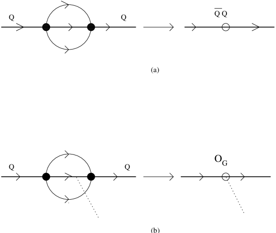
Figure 1.1: Perturbative corrections to the Transition operator, T, (left) and to the local operators in OPE (right). (a) $\bar{Q}Q$ (b) $\bar{Q}g\sigma GQ$ (Dotted lines are gluons).

Then the inclusive decay rate is given by these set of operators by

$$\Gamma(H_{Q}\rightarrow X)={G_{f}^{2}|V_{KM}|^{2}m_{Q}^{5}\over{192\pi^{3}}}\left(c_{3}\left<\bar{Q}Q\right>_{H}+c_{5}{\left<\bar{Q}g\sigma_{\mu\nu}G^{\mu\nu}Q\right>_{H}\over{m_{Q}^{2}}}+\cdots\right)$$ (1.79)

where $c_{n}$ are the short distance Wilson coefficients calculable in perturbation theory, and

$$\left<O\right>_{H}={1\over{2M_{H}}}\left<H_{Q}|O|H_{q}\right>$$ (1.80)

The hadronic matrix elements are expanded in inverse powers of the heavy quark mass (Figure 1.1) as

$$\left<\bar{Q}Q\right>_{H} = 1-{\mu_{\pi}^{2}(H)-\mu_{G}^{2}(H)\over{2m_{Q}^{2}}}+O(1/m_{Q}^{3})$$ (1.81)

$$\left<\bar{Q}g\sigma_{\mu\nu}G^{\mu\nu}Q\right>_{H} = 2\mu_{G}^{2}(H)+O(1/m_{Q}^{2})$$ (1.82)

where the HQET matrix elements are defined as

$$\mu_{\pi}^{2}(H) = {1\over{2M}}\left<H(v)|\bar{Q}(iD)^{2}Q|H(v)\right>$$ (1.83)

$$\mu_{G}^{2}(H) = {1\over{2M}}\left<H(v)|\bar{Q}{g\over 2}\sigma_{\mu\nu}G^{\mu\nu}Q|H(v)\right>$$ (1.84)

Hence, we have the decay rate of the form

$$\Gamma(H_{Q}\rightarrow X)={G_{f}^{2}|V_{KM}|^{2}m_{Q}^{5}\over{192\pi^{3}}}\left\{c_{3}\left(1-{\mu_{\pi}^{2}(H)-\mu_{G}^{2}(H)\over{2m_{Q}^{2}}}\right)+2c_{5}{\mu_{G}^{2}(H)\over{m_{Q}^{2}}}+\cdots\right\}$$ (1.85)

In the above equation, the leading order term corresponds to the free quark decay rate. At $O(1/m_{Q}^{2})$, the term $\mu_{\pi}^{2}(H)$ describes the motion of the heavy quark inside the hadron and the term $\mu_{G}^{2}(H)$ the hyperfine interaction. The kinetic term for a $B$ meson is estimated to be in the range of 0.1 to 0.5 GeV² [66, 67, 68, 77] and the latest value is given by

$$\mu_{\pi}^{2}(B)=-\lambda_{1}=0.3\pm 0.2~{}\mbox{GeV${}^{2}$}$$ (1.86)

For the $\Lambda_{b}$ baryon, it is obtained using the mass values of the hadrons from the following relation

$$(m_{\Lambda_{b}}-m_{\Lambda_{c}})-(\overline{m}_{B}-\overline{m}_{D})=[\mu_{\pi}^{2}(B)-\mu_{\pi}^{2}(\Lambda_{b})]\left({1\over{2m_{c}}}-{1\over{2m_{b}}}\right)+O(1/m_{Q}^{2})$$ (1.87)

where $\overline{m}_{B,D}$ are the spin-averaged masses of $B$ and $D$ mesons. The kinetic energy of a heavy quark inside a meson and a baryon differs by

$$\mu_{\pi}^{2}(B)-\mu_{\pi}^{2}(\Lambda_{b})=0.01\pm 0.03~{}\mbox{GeV${}^{2}$}$$ (1.88)

It should be noted that the bound on the two terms are model independent

$$\mu_{\pi}^{2}(B)>\mu_{G}^{2}(B)\approx 0.35~{}\mbox{GeV${}^{2}$}$$ (1.89)

On the other hand, the hyperfine interaction term is determined precisely from the difference between the masses of the vector and pseudoscalar mesons:

$$\mu_{G}^{2}(B)={3\over 4}(M_{B*}-M_{B})=0.12~{}\mbox{GeV${}^{2}$}$$ (1.90)

For baryons it vanishes except in the case of the $\Omega_{Q}$ baryon.

The phase space factors corresponding to the $C_{n}$ are given by

$$c_{3} = 1-8x+8x^{3}-x^{4}-12x^{2}\log x^{2}$$ (1.91)

$$c_{5} = (1-x)^{4}$$ (1.92)

where $x=m_{q}^{2}/m_{b}^{2}$, the mass ratio of the final state quark to the decaying quark. The leading order factor given in (1.91) is exact [69] and the other due to higher orders in (1.92) is known only partially [70].

The total decay rate scales like $m_{b}^{5}$. The leading order term corresponds to the free heavy quark decay rate. This is universal for all hadrons of a given flavour. The next-to-leading order terms appear at $O(1/m_{b}^{2})$. They describe the heavy quark motion inside the hadron and the hyperfine interaction due to heavy quark spin projection. However, the next to leading order contributions are suppressed by $m_{b}^{-2}$.

With these, the important predictions for inclusive properties of beauty hadrons are given in Table 1.4.

Table 1.4: HQE predictions vs Experimental Values

	theory	experiment
$\tau$$(B^{+})$/$\tau$$(B^{0}_{d})$	1+$O(1/m_{b}^{3})$	1.02 $\pm$0.04
$\tau$$(B^{0}_{s})$/$\tau$$(B^{0}_{d})$	(1.0 $\pm$ 0.01)+$O(1/m_{b}^{3})$	1.01 $\pm$0.07
$\tau$$(\Lambda_{b})$/$\tau$$(B^{0}_{0})$	0.98 + $O(1/m_{b}^{3})$	0.78 $\pm$0.05
$Br(B)_{SL}$	12.5%	10.5%
$n_{c}$	1.16	1.24

Because of the discrepancy in the case of $\Lambda_{b}$, the semileptonic branching ratio of $B$ mesons, $Br(B)_{SL}$ [73, 74, 75] and the charm counting, $n_{c}$, [72, 76], the third order in $1/m_{Q}$ terms have necessarily to be evaluated. This will be discussed in the next chapter.

Chapter 2 Four-quark operators

In this Chapter we discuss the evaluation of the expectation values of four-quark operators (EVFQO). The EVFQO are estimated in two different approaches: (1) in terms of the form factor characterising the light scattering off the heavy quark inside the hadron, using a potential model, and (2) from the difference in the total decay rates of beauty hadrons.

2.1 Preview

As already mentioned, in order to systematically accommodate the contribution coming from the terms at the third order of the heavy quark expansion, it is necessary to evaluate the expectation values of the four-quark operators. These are the dimension six operators involving both the heavy and light quark fields. Though their contributions are negligible as compared to the volume of heavy quark occupation, $O{(\Lambda_{QCD}/m_{Q})^{3}}$, they are considerably enhanced due to partial compensation by the four-quark phase-space. As previously noted, the lifetimes of all mesons as well as baryons are almost equal among themselves respectively. But the knowledge of their individual hierarchy depends on the outcome of the terms at $O(1/m_{Q}^{3})$. Besides, the persisting confrontation of the theoretical estimate of the lifetime of $\Lambda_{b}$ with the experimental value necessiates the evaluation of the four-quark operators.

The hadronic matrix elements at $O(1/m_{Q}^{3})$ is

$$C(\mu)\left<H_{b}|(\bar{Q}\Gamma_{\mu}Q)(\bar{q}\Gamma^{\mu}q)|H_{b}\right>$$ (2.1)

where $\Gamma_{\mu}$ stands for some arbitrary Dirac structure, the coefficient $C(\mu)$ describes the short distance QCD processes which will be discussed in the next chapter. The operators, in (2.1), are induced into a set of four by the spectator effects. They are:

$$O^{q}_{V-A} = \bar{b}\gamma_{\mu}(1-\gamma_{5})q\bar{q}\gamma^{\mu}(1-\gamma_{5})b$$ (2.2)

$$O^{q}_{S-P} = \bar{b}(1-\gamma_{5})q\bar{q}(1+\gamma_{5})b$$ (2.3)

$$T^{q}_{V-A} = \bar{b}\gamma_{\mu}(1-\gamma_{5})t^{a}q\bar{q}\gamma^{\mu}(1-\gamma_{5})t^{a}b$$ (2.4)

$$T^{q}_{S-P} = \bar{b}(1-\gamma_{5})t^{a}q\bar{q}(1+\gamma_{5})t^{a}b$$ (2.5)

By insertion of vacuum states, we have

$$\left<O^{q}_{V-A}\right>_{B_{q}} = \left<O^{q}_{S-P}\right>_{B_{q}}=f_{B}^{2}m_{B}^{2}$$ (2.6)

$$\left<T^{q}_{V-A}\right>_{B_{q}} = \left<T^{q}_{S-P}\right>_{B_{q}}=0$$ (2.7)

where $f_{B}$ is the leptonic decay constant of $B$ meson. The evaluation of the operators is a difficult task. It involves the nonperturbative aspect of QCD. The expectation values of these operators are understood as the probability of finding both the quarks at the origin, $|\Psi(0)|^{2}$. The traditional way of estimating the expectation values of these operators for a meson is to use the vacuum insertion approximation and express the value in terms of the leptonic decay constant:

$${1\over{2m_{B}}}\left<B|(\bar{Q}\Gamma_{\mu}Q)(\bar{q}\Gamma^{\mu}q)|B\right>=|\Psi(0)|^{2}_{B}={f_{B}^{2}m_{B}\over{12}}$$ (2.8)

On the other hand, for baryon, one has to use the valence quark approximation. These estimations are model dependent. We next discuss the evaluation of the expectation values of four-quark operators made by Rosner [81], Neubert and Sachrajda [82] and De Fazio and Colangelo[83], followed by the evaluation made in potential model and from the difference in the decay rates of the $SU(3)$ triplet mesons and baryons.

In [81], Rosner estimated the wavefunction density for $\Lambda_{b}$ in constituent model using the DELPHI value of mass difference between $\Sigma$ and $\Sigma^{*}$ [84]. With the four-quark operators of a meson estimated in terms of the leptonic decay constant, the operators of a baryon can be made in a quark model using the hyperfine mass splitting of the $b$-baryons. The mass splittings due to the hyperfine interaction in a meson, $M_{i\bar{j}}$, and in a baryon, $B_{ijk}$, are given by

$$\Delta M(M_{i\bar{j}}) = {32\pi\over 9}\alpha_{s}{\left<{\hat{s}}_{i}.{\hat{s}}_{j}\right>\over{m_{i}m_{j}}}|\Psi(0)|^{2}_{i\bar{j}}$$ (2.9)

$$\Delta M(B_{ijk}) = {16\pi\over 9}\alpha_{s}\sum_{i>j}{\left<{\hat{s}}_{i}.{\hat{s}}_{j}\right>\over{m_{i}m_{j}}}|\Psi(0)|^{2}_{ij}$$ (2.10)

The value of $\left<{\hat{s}}_{Q}.{\hat{s}}_{\bar{q}}\right>$ is (1/4, -3/4) for a $(^{3}S_{1},^{1}S_{0})$ $Q\bar{q}$ meson. With $S_{qq}=1$, $\left<{\hat{s}}_{Q}.{\hat{s}}_{\bar{q}}\right>$ is (1/4, -1/2) for states with total spin $(3/2,1/2)$ for a $Qqq$ baryon. With these, the expectation values of four-quark operators for a $b$-baryon is:

$$|\Psi(0)|^{2}_{\Lambda_{b}}={4\over 3}{\Delta B_{ijk}\over{\Delta M_{ij}}}|\Psi(0)|^{2}_{B}$$ (2.11)

For the baryon mass splitting, $M(\Sigma_{b}^{*})-M(\Sigma_{b})=56\pm 16$ MeV [84] and for $M(B^{*})-M(B)=46$ MeV, we get

$$|\Psi(0)|^{2}_{\Lambda_{b}}=(2.6\pm 1.3)\times 10^{-2}~{}~{}\mbox{GeV${}^{3}$}$$ (2.12)

As will be discussed in the next chapter, this value is found not sufficient to account for the smaller lifetime of $\Lambda_{b}$. However, this work is in favour of larger value of $|\Psi(0)|^{2}$ for $\Lambda_{b}$ than that of $B$.

Neubert and Sachrajda [82] parameterised the dimension six matrix elements in terms of hadronic parameters. The four-quark matrix elements between hadrons are given in terms of the hadronic parameters $B_{i},\epsilon_{i}$. For $B$ mesons

$${1\over{2m_{B}}}\left<B|(\bar{b}_{L}\gamma_{\mu}q_{L})(\bar{q}_{L}\gamma^{\mu}b_{L})|B\right>\equiv{f_{B}^{2}m_{B}\over 8}B_{1}$$ (2.13)

$${1\over{2m_{B}}}\left<B|(\bar{b}_{R}q_{L})(\bar{q}_{L}b_{R})|B\right>\equiv{f_{B}^{2}m_{B}\over 8}B_{2}$$ (2.14)

$${1\over{2m_{B}}}\left<B|(\bar{b}_{L}\gamma_{\mu}t^{a}q_{L})(\bar{q}_{L}\gamma^{\mu}t^{a}b_{L})|B\right>\equiv{f_{B}^{2}m_{B}\over 8}\epsilon_{1}$$ (2.15)

$${1\over{2m_{B}}}\left<B|(\bar{b}_{R}t^{a}q_{L})(\bar{q}_{L}t^{a}b_{R})|B\right>\equiv{f_{B}^{2}m_{B}\over 8}\epsilon_{2}$$ (2.16)

where the hadronic parameters in the large-$N_{c}$ limit

$$B_{i}=O(1),\hskip 14.22636pt\epsilon_{i}=O(1/N_{c})$$ (2.17)

Using QCD sum rules, it is found that $\epsilon_{1}=-0.15$ and $\epsilon_{2}=0$.

Similarly, the matrix elements between $\Lambda_{b}$ states are expressed as

$${1\over{2m_{\Lambda_{b}}}}\left<\Lambda_{b}|(\bar{b}_{L}\gamma_{\mu}q_{L})(\bar{q}_{L}\gamma^{\mu}b_{L})|\Lambda_{b}\right>\equiv-{f_{B}^{2}m_{B}\over 8}r$$ (2.18)

where $r={|\Psi(0)|^{2}_{\Lambda_{b}}/{|\Psi(0)|^{2}_{B}}}$. It is expected that the ratio is about unity. But Rosner argued that it should be larger than unity.

2.2 Potential Model Evaluation

In the nonrelativistic quark theory, the wave function density and diquark density are related to the associated operator

$$O_{6}=(\bar{b}_{i}\Gamma_{b}b^{i})(\bar{q}_{j}\Gamma_{q}q^{j}),$$ (2.19)

where the ${\Gamma_{b,q}}$ are arbitrary Dirac structures, through

$${1\over{2M_{B}}}<B|(\bar{b}b)(\bar{q}q)|B> = |\Psi(0)|^{2}$$ (2.20)

$${1\over{2M_{\Lambda_{b}}}}<{\Lambda_{b}}|(\bar{b}b)(\bar{q}q)|{\Lambda_{b}}> = \int d^{3}y|\Psi(0,y)|^{2}$$ (2.21)

for a meson and a baryon respectively. The operators in (2.19) are colour singlet. The expectation values of these operators are related to the transition amplitude of the light quark scattering off the heavy quark. Thus the determination is based on the knowledge of the light quark scattering form factor.

The wave function at the origin, in momentum representation, is given by

$$\Psi(0)=\int{d^{3}{\bf p}\over{(2\pi^{3})^{3}}}\Psi({\bf p}).$$ (2.22)

The transition amplitude is then the Fourier transform of the light quark density distribution:

$$F({\bf q})={1\over{2M_{H}}}<H_{b}({\bf q})|\bar{q}q(0)|H_{b}(0)>=\int d^{3}{\bf x}\Psi^{*}({\bf x})\Psi({\bf x})e^{i{\bf q}{\bf x}}.$$ (2.23)

Integrating over all q yields the expectation value:

$$\int{d^{3}{\bf q}\over{(2\pi)^{3}}}F({\bf q})=|\Psi(0)|^{2}={1\over{2M_{H}}}<H_{b}|\bar{b}b\bar{q}q(0)|H_{b}>$$ (2.24)

For any Dirac structure ${\Gamma}$, the light quark current density and the light quark transition amplitude are given by:

$$J_{\Gamma}({\bf x}) = \bar{q}\Gamma q({\bf x})$$ (2.25)

$$A_{\Gamma}({\bf q}) = {1\over{2M_{H}}}<H_{b}({\bf q})|J_{\Gamma}(0)|H_{b}(0)>$$ (2.26)

where the J_Γ(0) is gauge invariant operator, and it is not required to be a bilinear. Thus, for spin-singlet operators, we have

$$<H({\bf q})|\bar{b}bJ_{\Gamma}(0)|H_{b}(0)>=\int{d^{3}{\bf q}\over{(2\pi)^{3}}}<H_{b}({\bf q})|J_{\Gamma}(0)|H_{b}(0)>$$ (2.27)

And, similarly for spin-triplet operators,

$$<\ H({\bf q})|\bar{b}{\bf\sigma_{k}}b\bar{J}_{\Gamma}(0)|H_{b}(0)>=\int{d^{3}{\bf q}\over{(2\pi)^{3}}}<S_{k}\ H_{b}({\bf q})|J_{\Gamma}(0)|H_{b}(0)>$$ (2.28)

with S/2 being the b-quark spin operator and

$$|S_{k}\ H_{b}>=\int d^{3}{\bf x}\bar{b}\sigma_{k}b({\bf x})|\ H_{b}>$$ (2.29)

Equations (2.27) and (2.28) represent the general structure of four-quark operators. The above operators are local as required for by the HQE in the sense that the light quark operators enter at the same point as the heavy b-quark operators. These relations hold equally for different initial and final hadrons having different momenta smaller than m_b.

Equation (2.19) resolves into spin-singlet and spin-triplet operators for ${\Gamma_{b}}$ = 1 and ${\Gamma_{b}}$ = ${{\bf\gamma}\gamma_{5}(={\bf\sigma})}$ respectively. The light quark elastic scattering is described by the form factor F(q²). In Ref. [85], the exponential ansatz and the two pole ansatz are used for the form factor. Both of them lead to a result which is the same for meson and baryon.

Model for form factor

As will be discussed in the following sections, the expectation values of the colour-straight operators are parameterised in terms of a single form factor for both the B-meson and ${\Lambda_{b}}$ baryon [80]. The extraction of the form factor involves an assumption of a function such that it satisfies the constraints on the form factor that F(q² = 0) is equal to the corresponding charge of the hadron. Then the form factor has to be extrapolated into the region where q² ${>}$ 0. We take the hadronic wave function of ISGW harmonic oscillator model [86] for the form factor. The wave functions of ISGW model are the eigenfunctions of the orbital angular momentum L = 0 satisfying the overlapping integral which is chosen as the form factor.

$$F({\bf q}^{2})=N^{2}exp[-q^{2}/2(\beta_{f}^{2}+\beta_{i}^{2})]$$ (2.30)

where N is the normalisation constant given by ${[2\beta_{f}\beta_{i}/(\beta_{f}^{2}+\beta_{i}^{2})]^{3/2}}$ and ${\beta}$’s are oscillator strengths. For the same initial and final hadrons ($\beta_{i}=\beta_{f}=\beta$), the transition amplitude is [80]

$$\int{d^{3}{\bf q}\over{(2\pi)^{3}}}F(q^{2})={\beta^{3}\over{4\pi^{3/2}}}=|\Psi(0)|^{2}$$ (2.31)

From the above equation, which is the master equation for evaluation of the EVFQO, it is obvious that the transition amplitude and hence the expectation values of four fermion operators are proportional to the third power of the oscillator strength of the hadron.

The calculation of ${\beta}$’s can be made using a QCD inspired potential. In the present calculation, we use the potential for a B-meson containing the Coulomb, confining and constant terms:

$$V(r)={a\over{r}}+br+c$$ (2.32)

where a = – 0.508, b = 0.182 GeV² and c = – 0.764 GeV. With quark masses m_q = 0.3 GeV (treating m_u = m_d), m_s = 0.5 GeV and m_b = 4.8 GeV, using a variational procedure with the wave function given in position space as,

$$\Psi(0)_{1s}={\beta^{3/2}\over\pi^{3/4}}e^{-\beta^{2}r^{2}/2}$$ (2.33)

the oscillator strengths of the beauty mesons are obtained. The values are [86]

$${\beta}_{B_{q}}=0.4~{}\mbox{GeV}$$ (2.34)

$${\beta}_{B_{s}}=0.44~{}\mbox{GeV}$$ (2.35)

For the ${\Lambda_{b}}$ baryon, we use the same procedure as before but a potential of the form

$$V(r)={1\over{2}}\left({a\over{r}}+br+\zeta^{\prime}r^{2}+c\right)$$ (2.36)

where $\zeta^{\prime}=\zeta\beta^{2}$, with $\zeta=1$ GeV and the r² term is a harmonic oscillator term justifying the consideration that the ${\Lambda_{b}}$ be a two body system using the same wave function as in (2.33), we determine the values of $\beta$ for the baryons [80]:

$${\beta_{\Lambda_{b}}}=0.72~{}\mbox{GeV}$$ (2.37)

$${\beta_{\Xi_{b}}}=0.76~{}\mbox{GeV}$$ (2.38)

We have taken the mass of the diquark system as 0.6 and 0.8 GeV for $\Lambda_{b}$ and $\Xi_{b}$ respectively.

The large value for the $\beta_{\Lambda_{b}}$ is due to the presence of the O(r²) term in the potential. Otherwise, the value of $\beta_{\Lambda}$ is no different than that of B_s. These values are used in the subsequent calculations. A comment is in order on the choice of the same wave function for both the baryon as for meson: In the usual procedure, the ground state wave function for a baryon is

$$\Psi_{ground}\approx e^{-\alpha^{2}(r_{\lambda}^{2}+r_{\rho}^{2})/2}$$ (2.39)

where r_λ,ρ are the internal coordinates for the three body system. Due to the idea of considering ${\Lambda_{b}}$ as a system containing the bound state of light quarks and a heavy quark, the separation between the two light quarks which make the bound state, is treated negligible. Then the baryon can be considered as a two body system, a reasonable approximation. The difference between a meson and a baryon is essentially due to the value of the oscillator strength.

Expectation values

We evaluate the expectation values of the colour-straight operators only for the vector and axial-vector currents. Nevertheless, the other currents can also be studied in the same fashion. Both the currents are possible for the B-meson, while axial currents vanish for ${\Lambda_{b}}$ baryon due to the light quarks constituting a spinless bound state.

Essentially there is no difference between the exponential ansatz and the harmonic oscillator wave function in representing the behaviour of the form factor, but they differ while fixing the scale: in the former case, the hadronic scale of one GeV is used whereas in the latter the same has been fixed by solving the Schrödinger equation. The two pole anstaz is based on the well founded experimental values. Basically, the use of the harmonic oscillator wave function of the constituent quark model is an alternate picture but in the very same lines of the ansatz.

Hereinafter the operators are referred to by the following notation: for the meson

$$<O_{V,A}^{q}>_{H}=\left<\bar{b}\Gamma_{V,A}b\bar{q}\Gamma_{V,A}q\right>$$ (2.40)

$$<T_{V,A}^{q}>_{H}=\left<\bar{b}\Gamma_{V,A}t^{a}b\bar{q}\Gamma_{V,A}t^{a}q\right>$$ (2.41)

where $\Gamma_{V,A}=\gamma_{\mu},\gamma_{\mu}\gamma_{5}$ and ${t^{a}t^{b}=1/2-1/2N_{c}}$. In what follows, q stands for u and d quarks and s for the strange quark.

And, ${<O_{V,A}>,<T_{V,A}>}$ will be respectively denoted as ${\omega_{V,A},\tau_{V,A}}$. For the baryon, $<O(T)_{V}>$ correspond to $\lambda_{1,2}$ respectively.

B-meson

The parameterisation of the matrix element of the colour-straight operators for the vector current is

$$<B(q)|J_{\Gamma_{V}}|B(0)>=-v_{\mu}F_{B}(q^{2})$$ (2.42)

with the constraints F_B(0) = 1 for valence quark current and F_B(0) = 0 for the sea quark current. The former is relevant for the b-meson composition of quarks b${\bar{q}}$. Then the corresponding transition amplitude is

$$A_{\Gamma_{V}}^{B}=<B(q)|O_{V}^{q}|B(0)>=v_{\mu}\int{d^{3}q\over{(2\pi)^{3}}}F_{B}(q^{2})$$ (2.43)

Under isospin SU(2) symmetry,

$$\left<O_{V}^{q}\right>_{B^{-}}=2.88\times 10^{-3}~{}\mbox{GeV${}^{3}$}$$ (2.44)

$$\left<T_{V}^{q}\right>_{B^{-}}=9.61\times 10^{-4}~{}\mbox{GeV${}^{3}$}$$ (2.45)

For B_s, we have

$$\left<O_{V}^{q}\right>_{B_{s}}=3.83\times 10^{-3}~{}\mbox{GeV${}^{3}$}$$ (2.46)

$$\left<T_{V}^{q}\right>_{B_{s}}=1.28\times 10^{-3}~{}\mbox{GeV${}^{3}$}$$ (2.47)

If violation of isospin symmetry and SU(3) flavour symmetry is considered, then there comes Cabibbo mixing of eigenstates for d and s quarks among themselves. That is, $d^{\prime}=d\cos\theta_{c}+s\sin\theta_{c}$ and $s^{\prime}=s\cos\theta_{c}+d\sin\theta_{c}$. This would bring in negligible corrections.

For the axial current, there are two form factors which are related to each other due to the conservation of the axial current, ${{\partial_{\mu}}J_{\mu 5}}$ = 0, in the chiral limit. By the Goldberger-Treiman relation [87] which equates axial charge form factor to the coupling g${{}_{B^{*}B\pi}}$ at q² = 0, the operators involving the axial-currents are estimated in terms of a single form factor. Thus, given the value of the coupling g, the extraction of the transition amplitude is similar to the B-meson case.

With the Goldberger-Treiman relation, we obtain the EVFQO for axial currents as

$$G_{1}(q^{2})=q^{2}G_{0}(q^{2})=ge^{-q^{2}/4\beta^{2}}$$ (2.48)

where g = – 0.03 [88, 89]. The numerical estimates are

$$\left<O_{A}^{q}\right>_{B^{-}}=8.63\times 10^{-5}~{}\mbox{GeV${}^{3}$}$$ (2.49)

$$\left<T_{A}^{q}\right>_{B^{-}}=2.88\times 10^{-5}~{}\mbox{GeV${}^{3}$}$$ (2.50)

$$\left<O_{A}^{s}\right>_{B_{s}}=1.15\times 10^{-4}~{}\mbox{GeV${}^{3}$}$$ (2.51)

$$\left<T_{A}^{s}\right>_{B_{s}}=3.84\times 10^{-5}~{}\mbox{GeV${}^{3}$}$$ (2.52)

These values are insignificant as compared to the vector current contributions.

$\Lambda_{b}$ baryon

For the ${\Lambda_{b}}$ baryon, treating u and d quarks equally,

$$\left<O_{V}^{q}\right>_{\Lambda_{b}}=1.69\times 10^{-2}~{}\mbox{GeV${}^{3}$},\hskip 17.07182pt\left<T_{V}^{q}\right>_{\Lambda_{b}}=5.64\times 10^{-3}~{}\mbox{GeV${}^{3}$}$$ (2.53)

In the case of ${\Xi_{b}}$, we have,

$$\left<\sum_{q^{\prime}=u,d,s}O_{V}^{q^{\prime}}\right>_{\Xi_{b}}=2.01\times 10^{-2}~{}\mbox{GeV${}^{3}$},\hskip 17.07182pt\left<\sum_{q^{\prime}=u,d,s}T_{V}^{q^{\prime}}\right>_{\Xi_{b}}=6.72\times 10^{-3}~{}\mbox{GeV${}^{3}$}$$ (2.54)

Even though there are corrections to the form factors due to charge radius, they are ignored as we are interested in the wave function density at the origin.

Non-factorisable part of the FQO

The nonfactorisable parts of the FQO come in four. The following is one of the ways of parameterising them [82].

$${1\over{2M_{B}}}<B|(\bar{b}q)_{V-A}(\bar{q}b)_{V-A}|B>={\bar{f}_{B}^{2}}M_{B}B_{1}/2$$ (2.55)

$${1\over{2M_{B}}}<B|(\bar{b}t^{a}q)_{V-A}(\bar{q}t^{a}b)_{V-A}|B>={\bar{f}_{B}^{2}}M_{B}\epsilon_{1}/2$$ (2.56)

$${1\over{2M_{B}}}<B|(\bar{b}q)_{S-P}(\bar{q}b)_{S-P}|B>={\bar{f}_{B}^{2}}M_{B}B_{2}/2$$ (2.57)

$${1\over{2M_{B}}}<B|(\bar{b}t^{a}q)_{S-P}(\bar{q}t^{a}b)_{S-P}|B>={\bar{f}_{B}^{2}}M_{B}\epsilon_{2}/2$$ (2.58)

where $B_{1,2}$ and $\epsilon_{1,2}$ are hadronic parameters. They are related to $w_{V,A}$ and $\tau_{V,A}$ which are the expectation values of the operators $O_{V,A}$ and $T_{V,A}$ as defined earlier:

$${\bar{f}_{B}^{2}}M_{B}B_{1}=\phi_{1}=4(\tau_{V}+\tau_{A})+{2\over{N_{C}}}(\omega_{V}+\omega_{A})$$ (2.59)

$${\bar{f}_{B}^{2}}M_{B}B_{2}=\phi_{2}=-2(\tau_{V}-\tau_{A})-{1\over{N_{C}}}(\omega_{V}-\omega_{A})$$ (2.60)

$${\bar{f}_{B}^{2}}M_{B}\epsilon_{1}=\rho_{1}=-{2\over{N_{C}}}(\tau_{V}+\tau_{A})+(1-{1\over{N_{C}^{2}}})(\omega_{V}+\omega_{A})$$ (2.61)

$${\bar{f}_{B}^{2}}M_{B}\epsilon_{2}=\rho_{2}={1\over{N_{C}}}(\tau_{V}-\tau_{A})-{1\over{2}}(1-{1\over{N_{C}^{2}}})(\omega_{V}-\omega_{A})$$ (2.62)

In the case of the $\Lambda_{b}$ baryon, the nonfactorisable piece corresponds to [82]

$$<(\bar{b}q)_{V-A}(\bar{q}b)_{V-A)}=-{1\over{2N_{C}}}\lambda_{1}-\lambda_{2}$$ (2.63)

2.3 Flavour dependence of decay rates

In this section, we attempt to evaluate the expectation values of the four-quark operators from the differences in the total decay rates of the $b$-hadrons. That means we assume that the heavy quark expansion, being asymptotic in nature, converges at $O(1/m^{3})$ of the expansion. Already the next-to-leading order contribution due to terms of $O(1/m^{2})$ is only about five percent of the leading order. Thus, it cannot be anticipated that the size of the terms at the third order in $1/m$ would be more than a few percent. On the other hand, the observation made above is applicable only to the beauty case, since

$${16\pi^{2}\over{m_{c}^{3}}}C(\mu)\left<O_{6}\right>_{H_{c}}\gg{16\pi^{2}\over{m_{b}^{3}}}C(\mu)\left<O_{6}\right>_{H_{b}}$$ (2.64)

where $C(\mu)$ stands for some structure involving $c_{\pm}$ and $\left<O_{6}\right>_{H}$, the dimension six FQO of hadron. Hence, in the background described, we make use of the total decay rates to obtain the expectation values of the four-quark operators for the $b$-hadrons. Therefore, the present evaluation depends only on the heavy quark expansion and the $SU(3)$ flavour symmetry, as has been shown in [91].

Splitting of Decay Rates and Expectation Values of Four-quark Operators

The $B$ mesons, $B^{-}$, $B^{0}$ and $B^{0}_{s}$, are triplet under $SU(3)_{f}$ flavour symmetry. The total decay rate of $B$ meson splits up due to its light quark flavour dependence at the third order in the HQE. The differences in the decay rates of the triplet, $\Gamma(B^{0})-\Gamma(B^{-}),\Gamma(B^{0}_{s})-\Gamma(B^{-})$ and $\Gamma(B_{s}^{0})-\Gamma(B^{0})$, are related to the third order terms in $1/m$ by

$$\Gamma(B^{0})-\Gamma(B^{-}) = -\Gamma^{\prime}_{0}(1-x)^{2}\left\{Z_{1}{1\over 3}(2c_{+}-c_{-}+6)+2(c_{+}-c_{-}/2+1)\right\}$$ (2.65)

$$\times\left<O_{6}\right>_{B^{0}-B^{-}}$$

$$\Gamma(B^{0})-\Gamma(B^{-}) = -\Gamma^{\prime}_{0}(1-x)^{2}\left\{Z_{2}{1\over 3}(2c_{+}-c_{-}+6)+2(c_{+}-c_{-}/2+1)\right\}$$ (2.66)

$$\times\left<O_{6}\right>_{B^{0}_{s}-B^{-}}$$

$$\Gamma(B^{0})-\Gamma(B^{0}) = -\Gamma^{\prime}_{0}(1-x)^{2}\left\{(Z_{1}-Z_{2}){1\over 3}(2c_{+}-c_{-}+6)\right\}$$ (2.67)

$$\times\left<O_{6}\right>_{B^{0}_{s}-B^{0}}$$

where $\Gamma^{\prime}_{0}$ = $2G_{f}^{2}|V_{cb}|^{2}m_{b}^{2}/3\pi$, $c_{-}=c_{+}^{-2}=(\alpha(m)/\alpha(m_{W}))^{2\gamma/\beta},\beta=11-2n_{f}/3$ ($n_{f}$ the number of flavours), $\gamma=2$, $x$ = $m_{c}^{2}/m_{b}^{2}$ and

$$Z_{1} = \left(\cos^{2}\theta_{c}(1+{x\over 2})+\sin^{2}\theta_{c}\sqrt{1-4x}(1-x)\right)$$ (2.68)

$$Z_{2} = \left(\sin^{2}\theta_{c}(1+{x\over 2})+\cos^{2}\theta_{c}\sqrt{1-4x}(1-x)\right)$$ (2.69)

$$\left<O_{6}\right> = \left<{1\over 2}(\bar{b}\Gamma_{\mu}b)[(\bar{d}\Gamma_{\mu}d)-(\bar{u}\Gamma_{\mu}u)]\right>$$ (2.70)

$$\equiv\left<{1\over 2}(\bar{b}\Gamma_{\mu}b)[(\bar{s}\Gamma_{\mu}s)-(\bar{q}\Gamma_{\mu}q)]\right>$$

with $q=u,d$. In (2.65-2.67), the right hand side contains the terms corresponding to the unsuppresed and suppressed nonleptonic decay rates and twice the semileptonic decay rates at the third order.

For the decay rates $\Gamma(B^{-})=0.617$ ps^-1, $\Gamma(B^{0})=0.637$ ps^-1 and $\Gamma(B^{0}_{s})=0.645$ ps^-1 [2], the EVFQO are obtained for a $B$ meson, as an average from (2.65-2.67):

$$\left<O_{6}\right>_{B}=8.08\times 10^{-3}~{}\mbox{GeV${}^{3}$}.$$ (2.71)

This is smaller than the one obtained in terms of the leptonic decay constant, $f_{B}$.

On the other hand, for the triplet baryons, $\Lambda_{b}$, $\Xi^{-}$ and $\Xi^{0}$, with $\tau(\Lambda_{b})$ $<$ $\tau(\Xi^{0})\approx\tau(\Xi^{-})$, we have the relation between the difference in the total decay rates and the terms of $O(1/m^{3})$ in the HQE, as

$$\Gamma(\Lambda_{b})-\Gamma(\Xi^{0})={3\over 8}\Gamma_{0}^{\prime}(-c_{+}(2c_{-}+c_{+}-2)\left<O_{6}\right>_{\Lambda_{b}-\Xi^{0}}$$ (2.72)

We obtain the EVFQO for the baryon

$$\left<O_{6}\right>_{\Lambda_{b}-\Xi^{0}}=3.072\times 10^{-2}~{}\mbox{GeV${}^{3}$}$$ (2.73)

where we have used the decay rates corresponding to the lifetimes 1.24 ps and 1.39 ps [2] of $\Lambda_{b}$ and $\Xi^{0}$ respectively. The EVFQO for the baryon is about 3.8 times larger than that of the B meson. But it is about 3.5 - 4.0, depending on the changes in the mass and other sources of uncertainty.

The expectation values for a baryon is quite large. In fact, Rosner [81] found it to be 1.8 times larger than that of a meson which accounts for about 45% (if hard gluon exchange is included) of the needed enhancement in the decay rate. However, what we obtain is model independent. We have only used the experimental total decay rates. The result is surprising as well as genuine, if one has to believe the experimental values used. Still, there is room for uncertainty of a few percent. On the other hand, the generic structure we employed can be decomposed into many as found in [82] by Neubert and Sachrajda. Using them. we will get an improved estimate, but in that case it may become somewhat model dependent. We should note here that preliminary study on lattice [92] shows that the EVFQO would enhance the decay rate of $\Lambda_{b}$.

Chapter 3 Spectator effects

In this Chapter, we present the predictions for the ratio of lifetimes of beauty hadrons using the expectation values obtained in Ref. [80, 90]. Also presented is the determination the inclusive charmless semileptonic decay rate of $\Lambda_{b}$ and discuss its influence on $Br(b\rightarrow X_{u}l\nu)~{}$.

3.1 Spectator Processes

In the description of the inclusive decays of heavy hadrons by the heavy quark expansion, the total decay rate scales like $m_{b}^{5}$. Corrections appear at $O(1/m_{b}^{2})$ due to the heavy quark motion inside the hadron and the hyperfine interaction due to the heavy quark spin orientation. These corrections are about 10% of the leading order. As the heavy quark mass increases, the corrections are much suppressed by the inverse powers of the heavy quark mass. At the third order in $1/m_{b}^{3}$, the effects are due to the participation of the light quarks (See Figure3.1). Though the effects are negligibly small, they distinguish the lifetimes of various hadrons of given flavour quantum number. We discuss first the processes involving light quarks [93, 94, 95, 96]. Then we will use the expectation values of the four-quark operators of mesons and baryons estimated in the previous chapter to get the lifetimes of the beauty hadrons.

Pauli interference (PI)

For the decay of a $(Q\bar{q})$ hadron, the quark level process is $Q(q_{i})\rightarrow Q^{\prime}q_{f}q_{f}^{\prime}(q_{i})$, where the subscript associated with $q$’s denote the light quark in the initial hadron $i$ and the light quarks produced in the decay $f$. If one of the final state light quarks happens to be the same as the initial state quark, then the wave functions will interfere. For example consider the decay mode $B^{-}\rightarrow X_{c}X_{q}$, where the subscripts $c$ and $q$ denote the charmed and light quark of either $u$ and $d$ final states. If either of the light quarks in the final state $X_{q}$ is identical to the one in the initial hadron, they will interfere destructively. On the other hand, if $Q^{\prime}$ happens to be identical to $q_{i}$, then the interference will be a constructive one. The former will decrease the decay rate causing increase in the lifetime, while the latter will do the opposite.

The constructive interference can happen only in the baryon. For example, in the charmless semileptonic processes of $\Lambda_{b}\rightarrow X_{u}l\nu$, the corresponding quark process is $b(ud)\rightarrow X_{u}l\nu(ud)$. The $u$ quark in the state $X_{u}$ and the $u$ in the initial hadron will interfere constructively. This can happen in the nonleptonic process as well.

$W$-scattering (WS) and weak annihilation (WA)

Another spectator process corresponds to the cross-channel of the quark decay. In the notation used before, the light quark in the initial hadron can scatter off the heavy quark through exchange of $W$ field into a pair of light quarks, i. e., $q_{i}Q\rightarrow q_{f}q_{f}^{\prime}$. This process can happen only in baryons. This process is known as $W$-scattering or $W$-exchange, which occur in baryons only.

Or, if the quark scattering off the heavy one happens to be an anti-quark, then they annihilate into a pair of leptons or quarks via a $W$ boson: $q_{i}Q\rightarrow q_{f}~{}q_{f}^{\prime}$, where $q_{i}$ is an anti-quark. This is the so-called weak annihilation process occuring only in mesons.

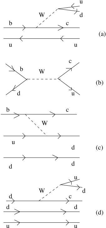
Figure 3.1: Spectator quark processes. (a) Pauli interference in B, (b) Weak annihilation in B, (c) W-scattering in $\Lambda_{b}$ and (d) Pauli interference in $\Lambda_{b}$.

3.2 Decay Rates due to Spectator Effects

We summarise below the spectator contribution to the beauty hadron decays.

The quark level process $b\rightarrow c\bar{u}d$:

• $B^{-}(b\bar{u})$: the $\bar{u}\bar{u}$ interference term is given by

  $$\Delta\Gamma(B^{-})=\Gamma_{0}24\pi^{2}C_{0}{<O_{6}^{q}>_{B^{-}}/{m_{b}^{3}}}$$ (3.1)

  where

  $$C{{}_{0}} = {c_{+}^{2}-c_{-}^{2}+(c_{+}^{2}+c_{-}^{2})/N_{c}}$$ (3.2)

  $${\Gamma_{0}} = G_{f}^{2}m_{b}^{5}|V_{KM}|^{2}/192\pi^{3}$$ (3.3)

  $$c_{+}=c_{-}^{-1/2} = (\alpha(m_{b})/\alpha(m_{W}))^{4/\beta_{0}}$$ (3.4)

  with $\beta_{0}=11-2n_{f}/3,n_{f}$ being the number flavours. In (3.1), $\left<O_{6}\right>$ stands for the EVFQO.

• $B^{0}_{d}(b\bar{d})$: In this case, the $d\bar{d}$ annihilation contributes to the total decay rate. The magnitude of this effect is not significant.

• $B_{s}^{0}(b\bar{s})$: No spectator effect occurs.

The spectator effects become significant depending on the quark level process.

For the above quark level process, in the case of beauty baryons, we have:

• $\Lambda_{b}(bud)$: There are two processes, $dd$ destructive Pauli interference and $u\bar{u}$ W-scattering. The Pauli interference in this case enhances the decay rate resulting in the $\Lambda_{b}$ lifetime smaller than the average lifetime of the beauty hadrons. The combined decay rates are given in (3.14 and 3.15) in the latter part of this Chapter.

• $\Xi^{0}(bds),\Xi^{-}(bus)$: In the case of these hyperons, weak scattering and destructible Pauli interference occur.

3.3 Lifetimes of Beauty Hadrons

Using the results obtained for the expectation values of the four-quark operators of the hadrons, we present the results for the ratio of lifetimes of them.

The decay rates of the b-flavoured hadrons are given by

$$\Gamma(H_{b}\rightarrow H_{c}l\bar{\nu}_{l})=\Gamma_{0}\left[(1-{\lambda_{1}-3\lambda_{2}\over{2m_{Q}^{2}}})f(x)+{2\lambda_{2}\over{m_{Q}^{2}}}f^{\prime}(x)\right]$$ (3.5)

where, with $x=m_{c}^{2}/m_{b}^{2}$

$$f(x) = 1-8x+8x^{3}-x^{4}+12x^{2}\mbox{ln}x^{2}$$ (3.6)

$$f^{\prime}(x) = (1-x)^{4}$$ (3.7)

are the QCD phase space factors and $\lambda_{1}$ and $\lambda_{2}$ correspond to the motion of the heavy quark inside the hadron and the chromomagnetic interaction respectively. We use: $\lambda_{1}(B)=0.5$ GeV², $\lambda_{1}(\Lambda_{b})=-0.43$ GeV² and $\lambda_{2}(B)=0.12$ GeV². Equation (3.5) is further supplemented by the FQO at the order (1/m${}_{Q}^{3}$) in the HQE.

3.3.1 Ratio of Lifetimes of B^- and B_d

Although the difference between the lifetimes of the charged and the neutral B-mesons is almost a settled issue, we check them once again using the expectation values of the colour-straight operators. This difference is attributed to PI and WA. Neglecting the WA as it is strongly CKM suppressed the result for the PI is

$$\Delta\Gamma^{f}(B^{-})=\Gamma_{0}24\pi^{2}C_{0}{<O_{V}^{q}>_{B^{-}}-<O_{A}^{q}>_{B^{-}}\over{m_{b}^{3}}}$$ (3.8)

where C₀ = ${c_{+}^{2}-c_{-}^{2}+{1\over{N_{c}}}(c_{+}^{2}+c_{-}^{2})}$ and the values for Wilson coefficients are: c₊ = 0.84 and c_– = -1.42 with N_c = 3. We use m_b = 4.8 GeV and ${|V_{cb}|}$ = 0.04. Then the ratio is

$${\tau(B^{-})\over{\tau(B_{d})}}=1.00$$ (3.9)

This agrees well with the one obtained in terms of B-meson decay constants.

The decay rates due to spectator quark(s) processes are: For B^-,

$$\Delta\Gamma^{nf}(B^{-})={G_{f}^{2}m_{b}^{2}\over{12\pi}}|V_{cb}|^{2}(1-x)^{2}[(2c_{+}^{2}-c_{-}^{2})\phi_{1}+3(c_{+}^{2}+c_{-}^{2})\rho_{1}]$$ (3.10)

Hence the ratio is 1.03.

3.3.2 Ratio of Lifetimes of B^- and B_s

The difference in lifetimes between the two neutral mesons B_s and B_d is due to $W$ exchange. The numerical result is

$${\tau(B_{s})\over{\tau(B_{d})}}=1.00$$ (3.11)

Corresponding to the nonfactorisable part, we get the decay rate

$$\Delta\Gamma^{nf}(B_{s})={\overline{\Gamma}_{0}}(1-4x)^{1/2}\eta$$ (3.12)

where $\overline{\Gamma}_{0}={G_{f}^{2}m_{b}^{2}/{12\pi}}|V_{cb}|^{2}$ and $\eta$ is given by

$$\eta={(2c_{+}-c_{-})^{2}\over{3}}\left[((1-x)\phi_{1}^{s}-(1+2x)\phi_{2}^{s})+{(c_{+}+c_{-})^{2}\over{2}}((1-x)\rho_{1}^{s}-(1+2x)\rho_{2}^{s})\right]$$ (3.13)

The ratio becomes 1.02.

3.3.3 Ratio of Lifetime of ${\Lambda_{b}}$ and B^-

In the HQE, the difference in lifetimes between mesons and baryons begins to appear at order 1/m${}_{Q}^{2}$. Nevertheless, it is dominant at third power in 1/m_Q. At this order, the FQO receives corrections due to WS and PI. They are

$$\Gamma_{WS}(\Lambda_{b})=92\pi^{2}\Gamma_{0}c_{-}^{2}{<O_{V}^{q}>_{\Lambda_{b}}\over{m_{b}^{3}}}$$ (3.14)

$$\Gamma_{PI}(\Lambda_{b})=-48\pi^{2}\Gamma_{0}C_{1}{<O_{V}^{q}>_{\Lambda_{b}}\over{m_{b}^{3}}}$$ (3.15)

where $C_{1}=-c_{+}(2c_{-}-c_{+})$. As mentioned earlier, PI is destructible for radiative corrections and it enhances the decay rate leading to smaller lifetime for ${\Lambda_{b}}$. The effect of WS, on the other hand, is colour enhanced and its consequence is smaller. Hence,

$${\tau(\Lambda_{b})\over{\tau(B^{d})}}=0.79$$ (3.16)

The decay rate modified by the nonfactorisable piece is given by

$$\Delta\Gamma(\Lambda_{b})={G_{f}^{2}m_{b}^{2}\over{16\pi}}\bar{\lambda}[4(1-x)^{2}(c_{-}^{2}-c_{+}^{2})-(1-x)^{2}(1+x)(c_{-}-c_{+})(5c_{+}-c_{-})]$$ (3.17)

Correspondingly, the ratio is

$${\tau(\Lambda_{b})\over{\tau(B^{-})}}=0.84$$ (3.18)

In mesonic cases, the nonfactorisable piece gives a little higher value. In particular, the ratio of the lifetimes of the baryon and meson is significantly larger.

3.4 Inclusive Charmless Semileptonic Decay

Motivation

Precise determination of the CKM matrix elements is fundamentally an important task for the Standard Model. There are as many as five of the nine elements of the CKM matrix that can be extracted from the knowledge of the weak decays of beauty hadrons. Particularly, $|V_{cb}|$ and $|V_{ub}|$ can be extracted in the framework of heavy quark expansion (HQE) in a direct and fairly model independent way [21]. With the measurements of the inclusive charmless semileptonic branching ratio of $b$ hadrons by the ALEPH [98], L3 [99] and DELPHI [100] collaborations at LEP, the determination of $|V_{ub}|$ has attracted renewed interest recently. The measured values of inclusive charmless semileptonic branching ratio of $b$ hadrons and the corresponding values of $|V_{ub}|$ extracted are

$$Br(b\rightarrow X_{u}l\nu_{l}) = (1.73\pm 0.55\pm 0.55)\times 10^{-3},$$

$$|V_{ub}| = (4.16\pm 1.02)\times 10^{-3}\hskip 14.45377pt~{}\mbox{(ALEPH)}$$ (3.19)

$$Br(b\rightarrow X_{u}l\nu_{l}) = (3.3\pm 1.0\pm 1.7)\times 10^{-3},$$

$$|V_{ub}| = (6.0^{+0.8+1.4}_{-1.0-1.9}\pm 0.2)\times 10^{-3}.\hskip 50.58878pt~{}\mbox{(L3)}$$ (3.20)

$$Br(b\rightarrow X_{u}l\nu_{l}) = (1.57\pm 0.35\pm 0.48\pm 0.27)\times 10^{-3},$$

$$|{V_{ub}/{V_{cb}}}| = (0.103^{+0.011}_{-0.012}\pm 0.016\pm 0.010).\hskip 7.22743pt~{}\mbox{(DELPHI)}$$ (3.21)

In these analyses, the measured quantity is

$${Br(b\rightarrow ue\nu)\over{Br(b\rightarrow ce\nu)}}\propto\left|{V_{ub}\over{V_{cb}}}\right|^{2}\,.$$ (3.22)

This has an advantage of being free of many hadronic uncertainties that occur in the non-leptonic decays. Also, the determination of the CKM matrix elements from inclusive decays can in general be made with less theoretical uncertainties than the ones extracted from exclusive modes. For semileptonic decays of baryons, however, there could still be large spectator effects due to Pauli interference as pointed out by Voloshin for $\Xi_{c}$ [101]. To the inclusive charmless semileptonic branching ratio of $b$ hadrons, the contribution of $\Lambda_{b}$ is about 10% with the rest coming from the $B$ mesons. There are many theoretical works [102] which study the $B\rightarrow X_{u}l\nu_{l}$ to determine $|V_{ub}|$. But not much has been done on the inclusive charmless semileptonic decay of $\Lambda_{b}$. In the analyses of ALEPH and L3, $\Lambda_{b}\rightarrow X_{u}l\nu_{l}$ is included in their sample, but in that of DELPHI, the rejection of kaons and protons that was used in the selection criteria reduces the contributions from $\Lambda_{b}$.

We study the inclusive charmless semileptonic decay of $\Lambda_{b}$ [97]. We find that the baryonic decay rate is larger by a factor of about 1.36, due to spectator effects, than that of the $b$ quark decay rate. We then discuss the correction factors needed on $Br(b\rightarrow ul\nu_{l})$ to account for the spectator effect in $\Lambda_{b}\rightarrow X_{u}l\nu_{l}$.

3.4.1 Inclusive Charmless Semileptonic Decay Rates

The total rate of inclusively decaying beauty hadrons into a charmless final state is given by the HQE[21] as

$$\Gamma(H_{b})={G_{f}^{2}|V_{ub}|^{2}m^{5}\over{192\pi^{3}}}\left(1-{\lambda_{1}-3\lambda_{2}\over{2m^{2}}}-2{\lambda_{2}\over{m^{2}}}+O\left(1\over{m^{3}}\right)\right)$$ (3.23)

where, with $m$ being the mass of the heavy quark, the term of $O(1/m^{0})$ corresponds to the free heavy quark decay rate, the terms at $O(1/m^{2})$ describe the motion of the heavy quark inside the hadron ($\lambda_{1}$ = $-$0.5 GeV² for $B$ and $-$0.43 GeV² for $\Lambda_{b}$) and the chromomagnetic interaction due to the heavy quark spin projection ($\lambda_{2}$ = 0.12 GeV²) which vanishes for baryons except $\Omega_{Q}$ and the third order term in $1/m$ is given by

$C(\mu)\left<H|(\bar{b}\Gamma q)(\bar{q}\Gamma b)|H\right>$.

The operators in $\left<...\right>$, denoted as $\left<O_{6}\right>$ below, are evaluated in [103] by one of us for $B$ and $\Lambda_{b}$. The Wilson coefficients are describing the spectator quark processes like Pauli interference, weak annihilation and $W$-scattering which occurs in baryons only.

In the mode $\Lambda_{b}\rightarrow X_{u}l\nu_{l}$, the spectator effect is the constructive interference of the $u$ quark of the final state with the $u$ quark in the initial hadron (see Fig. LABEL:fg:diag) which enhances considerably the decay rate. Otherwise, without spectator effects, the baryonic decay rate is almost the same as that of the heavy quark decay rate. The decay rate due to spectator processes is given by

$${\Delta\Gamma(\Lambda_{b})=48\pi^{2}\Gamma_{0}{\left<O_{6}\right>_{\Lambda_{b}}\over{m^{3}}}}$$ (3.24)

where $\Gamma_{0}=G_{f}^{2}|V_{ub}|^{2}m^{5}/192\pi^{3}$. Using the expectation values of the four-quark operators obtained in Ref. [103] for $\Lambda_{b}$, $\left<O_{6}\right>_{\Lambda_{b}}=6.75\times 10^{-2}$ GeV³, we obtain the ratio

$${{\Gamma(\Lambda_{b}\rightarrow X_{u}l\nu_{l})}\over{\Gamma(b\rightarrow X_{u}l\nu_{l})}}=1.36.$$ (3.25)

whereas at $O(1/m^{2})$, this ratio is 1.01. It should be pointed out that this enhancement has a large theoretical uncertainty which is difficult to estimate. On the other hand, no such enhancement exists for $\Lambda\rightarrow X_{c}e\nu_{e}$ and thus the ratio is increased by 36% for $\Lambda_{b}$. In passing, we note that the hadronic $b\rightarrow u$ decay of $\Lambda_{b}$ is not substantially enhanced due to the cancellations of constructive $uu$ and destructive $dd$ interferences.

3.4.2 $Br(b\rightarrow X_{u}l\nu)$ and $V_{ub}$

The inclusive charmless semileptonic branching ratio of $b$ hadrons is given by

$$Br(b\rightarrow X_{u}l\nu_{l})=(1-f_{\Lambda_{b}})\Gamma(B\rightarrow X_{u}l\nu_{l})\tau(B)+f_{\Lambda_{b}}\Gamma(\Lambda_{b}\rightarrow X_{u}l\nu_{l})\tau(\Lambda_{b})$$ (3.26)

In principle, $\Xi_{b}^{0,-1}$ can also be produced at LEP. However, it is suppressed by $s\bar{s}$ production from vacuum relative to $u\bar{u}$ or $d\bar{d}$ production. Furthermore, the neutral $\Xi_{b}$ which consists of $b$, $u$, and $s$ quarks has the same enhancement factor as $\Lambda_{b}$ in the charmless semileptonic decay rate, even though the charged $\Xi_{b}$ which is made of $bds$ quarks does not have the corresponding enhancement. We will thus assume in this analysis that all weakly decaying b-baryons are $\Lambda_{b}$’s. Thus using the above estimate with $f_{\Lambda_{b}}$ = 10%, $\tau(B)$ = 1.64 ps and $\tau(\Lambda_{b})$ = 1.24 ps, we obtain the following value for inclusive charmless semileptonic branching ratio of $b$ hadrons:

$$Br(b\rightarrow X_{u}l\nu_{l})=1.16\times 10^{-3}$$ (3.27)

If the spectator effects are not included, then

$$Br(b\rightarrow X_{u}l\nu_{l})=1.13\times 10^{-3}$$ (3.28)

In the above estimate in Eqs. (3.25-3.28), we have employed $|V_{ub}|=3.3\times 10^{-3}$ and $m$ = 4.5 GeV. Also, we have used the decay rate for $B$ mesons as estimated at $O(1/m^{2})$ using the Eq. (3.23), $Br(B\rightarrow X_{u}l\nu_{l})=1.155\times 10^{-3}$. No spectator effect occurs in $b\rightarrow ul\nu$ transition in $B$ mesons except the negligible weak annihilation in $B^{-}$. Also, the experimental selection criteria used for the $X_{u}$ system mostly reject such final states.

The corrections on $|V_{ub}|$ due to the enhancement of $\Lambda_{b}\rightarrow X_{u}l\nu_{l}$ is about $-$1.3%, and with these corrections, the central values for $|V_{ub}|$ by ALEPH and L3 become, as given by $|V_{ub}|=\left({Br_{expt}/{Br_{theory}}}\right)^{1/2}0.0033$, as

$$|V_{ub}|=\left\{\begin{array}[]{ll}4.03\times 10^{-3}&\mbox{(ALEPH)}\\ 5.57\times 10^{-3}&\mbox{(L3)}\end{array}\right.$$

Finally, we observe that (1) the contribution of $\Lambda_{b}$ definitely influences the branching ratio due to a constructive Pauli interference and (2) such spectator effects in $\Lambda_{b}$ decay have to be taken into account for a precise determination of $|V_{ub}|$ which relies on charmless semileptonic decays.

Chapter 4 Short distance nonperturbative corrections

In this Chapter, we discuss the power corrections to the parton decay rate, due to renormalons, of the heavy hadron decays .

4.1 Renormalons

As early as 1952, Dyson [104] showed that the perturbative expansion in a renormalisable theory like QED is not convergent. It is also true in QCD. This issue poses an important conceptual problem of giving a meaning to perturbation theory. Dyson’s arguement is the following. An observable in QED, $F(e^{2})$ is expressed in an expansion in $e^{2}$ as

$$F(e^{2})=f_{1}e^{2}+f_{2}e^{4}+\cdots$$ (4.1)

If there is a radius of convergence around $e^{2}=0$, then there will be a convergent result also for $-e^{2}$. The latter corresponds to an attractive force of equal charges and a repulsive force of opposite charges. This would physically mean that the state corresponding to the equal charges has unbounded negative energy. Thus the perturbative series cannot converge for negative $e^{2}$. Hence the radius of convergence is zero.

The divergent series can be dealt by the Borel summation technique [105, 106]. A divergent perturbation series

$$f[a]=\sum_{n=1}^{\infty}f_{n}a^{n}=f_{1}a+f_{2}a^{2}+\cdots$$ (4.2)

can be re-expressed by the Borel transform $B[b]$.

$$B[b]=\sum_{n=0}^{\infty}f_{n+1}{b^{n}\over{n!}}\approx f_{1}+f_{2}b+f_{3}{b^{2}\over 2}+\cdots$$ (4.3)

The original series $F[a]$ can be reproduced by

$$f[a]=\int_{0}^{\infty}db~{}e^{-b/a}B[b]$$ (4.4)

This would give a meaning to the series $f[a]$ by the fact that the integral converges and $B[b]$ has no singularities in the integration range.

To be more explicit, let us consider

$$\int d^{4}x~{}e^{iqx}\left<0|T\{j_{\mu}(x)j_{\nu}(0)\}|0\right>=(g_{\mu\nu}q^{2}-q_{\mu}q_{\nu})\Pi(q^{2})$$ (4.5)

With $s=q^{2}$, the Adler function is defined as

$$D(s)=-s{d\over{ds}}\Pi(s)$$ (4.6)

For the case of QED or QCD, we consider

$$D_{n}(Q^{2})=\int d^{4}k~{}F(k^{2},kq,Q^{2}){a\over{k^{2}}}(blob)^{n}$$ (4.7)

where we defined $a=\alpha(Q62)/\pi$ and $(blob)^{n}$ represents $n$ loops in a gluons line (Figure 4.1). Then the above equation would have the form

$$D_{n}(Q^{2})=\int dk^{2}~{}k^{2}\Phi\left({k^{2}\over{Q^{2}}}\right){q\over{k^{2}}}\left[\beta a\log\left({k^{2}\over{Q^{2}}}\right)\right]^{n}$$ (4.8)

where $\beta$ is the first coefficient of the beta function. Finally, for momenta above and below $Q^{2}$, we have the expressions corresponding respectively to the ultraviolet and infrared regions:

$$D(Q^{2})_{UV}={Q^{2}\over{n+1}}\int_{0}^{\infty}db~{}e^{-b/a}{1\over{\beta{b\over{n+1}}}}$$ (4.9)

$$D(Q^{2})_{IR}={Q^{2}\over{m-1}}\int_{0}^{\infty}db~{}e^{-b/a}{1\over{\beta{b\over{m-1}}}}$$ (4.10)

Figure 4.1: Renormalon graph (dotted lines are gluons).

where $b=a\log(Q^{2}/k^{2})(h+1)$ with $h=m,n$.

In the infra red case, (4.9), the poles in the Borel plane correspond to $b=-(n+1)/\beta$ on the negative axis. Hence the poles are not in the integration range. Thus the poles are at $b=-2/\beta,-3/\beta,\cdots$. For the ultraviolet case, (4.10), the poles are at $b=+1/\beta,+2/\beta,\cdots$. In this case, $b=(m-1)a\log(k^{2}/Q^{2})$. Thus, in this case, poles are in the range of integration and hence they are Borel summable.

In the case of QCD which is asymptotically free in the UV region, the IR and UV renormalons defined above are interchanged. That is, the UV poles are at $b=-1/\beta,-2/\beta,\cdots$ and the IR poles at $b=+2/\beta,+3/\beta,\cdots$.

Operator Product Expansion

The divergence of perturbation theory is deeply connected with the operator product expansion (OPE). Consider the OPE

$$D(Q^{2})=[\mbox{parton model}](1+a_{1}\alpha(Q^{2})+a_{2}\alpha(Q^{2})^{2}+\cdots)+\sum_{n=4,6,...}C_{n}\left<O_{n}\right>$$ (4.11)

where $C$ stands for the coefficient functions, $\left<O_{n}\right>$ the operators of dimension $n$. We cannot have a dimension two operators. So the term $O(1/Q^{2})$ is absent. The perturbative part of the OPE receives the renormalon corrections [12]. It has been shown that the absence of the first power suppressed term corresponds to the absence of singularity at $b=+1/\beta$ in the Borel plane. However, the renormalon corrections to the perturbative series have one-to-one correspondence with the power suppressed terms.

4.2 Power Corrections

The divergence of the perturbation theory at large order brings in an ambiguity to physical quantities specified at short distances. According to the present understanding, the ambiguity is given by a class of renormalon diagrams which are chain of $n$-loops in a gluon line. The phenomenon is deeply connected with the operator product expansion (OPE). The perturbative part of the OPE receives the renormalon corrections [12]. Since in the OPE the first power-suppressed nonperturbative term is absent and the renormalon corrections constitute short distance nonperturbative effect, they are more significant than large order corrections.

The phenomenology of the power corrections is significant for the heavy quark expansion (HQE) to describe the inclusive decays of heavy hadrons by an expansion in the inverse powers of the heavy quark mass, $m_{Q}$. As the inclusive decay rate of heavy hadrons scales like the fifth power of the heavy quark mass, the power corrections arise due to momenta smaller than the heavy quark mass. However, these IR renormalons would, being nonperturbative effect, have greater influence in the HQE prediction of quantities of interest. These short distance nonperturbative effects can be sought for explaining the smaller lifetime of $\Lambda_{b}$. We should note that these power corrections to heavy quark decay rate represents the breakdown of the quark-hadron duality. Therefore, it may shed light on the working of the assumption of quark-hadron duality in the heavy quark expansion.

In this section, we study the renormalon corrections considering the heavy-light correlator in the QCD sum rules approach, assuming that the nonperturbative short distance corrections given by the gluon mass are much larger than the QCD scale. We carry out the analysis for both heavy meson and a heavy baryon. Our study shows that the short distance nonperturbative corrections to the baryon and the meson differ by a small amount which is significant for the smaller lifetime of the $\Lambda_{b}$.

Let us consider the correlator of hadronic currents $J$:

$$\Pi(Q^{2})=i\int d^{4}xe^{iqx}\left<0|T\{J(x)J(0)\}|0\right>$$ (4.12)

where $Q^{2}=-q^{2}$. The standard OPE is expressed as

$$\Pi(Q^{2})\approx[~{}\mbox{parton model}](1+a_{1}\alpha+a_{2}\alpha^{2}+....)+O(1/Q^{4})$$ (4.13)

where the power suppressed terms are quark and gluon operators. The perturbative series in the above equation can be rewritten as

$$D(\alpha)=1+a_{0}\alpha+\sum_{n=1}^{\infty}a_{n}\alpha^{n}$$ (4.14)

where the term in the sum is considered to be the nonperturbative short distance quantity. It is studied by Chetyrkin et al [107] assuming that the short distance tachyonic gluon mass, $\lambda^{2}$, imitates the nonperturbative physics of the QCD. This, for the gluon propagator, means:

$$D_{\mu\nu}(k^{2})={\delta_{\mu\nu}\over{k^{2}}}\rightarrow\delta_{\mu\mu}\left({1\over{k^{2}}}+{\lambda^{2}\over{k^{4}}}\right)$$ (4.15)

The nonperturbative short distance corrections are argued to be the $1/Q^{2}$ correction in the OPE.

Let us consider the assumption of the gluon mass $\lambda^{2}\gg\Lambda_{QCD}^{2}$ which is not necessarily to be tachyonic one. The feature of the assumption can be seen with the heavy quark potential

$$V(r)=-{4\alpha(r)\over{3r}}+kr$$ (4.16)

where $k\approx$ 0.2 GeV², representing the string tension. It has been argued in [108] that the linear term can be replaced by a term of order $r^{2}$. It is equivalent to replace $k$ by a term describing the ultraviolet region. For the potential in (4.16),

$$k\rightarrow constant\times\alpha\lambda^{2}$$ (4.17)

In replacing the coefficient of the term of $O(r)$ by $\lambda^{2}$, we make it consistent by the renormalisation factor. Thus the coefficient $\sigma(\lambda^{2})$ is given by [109]:

$$\sigma(\lambda^{2})=\sigma(k^{2})\left(\alpha(\lambda^{2})\over\alpha(k^{2})\right)^{18/11}$$ (4.18)

Introduction of $\lambda^{2}$ brings in a small correction to the Coulombic term. By use of (4.18), we specify the effect at both the ultraviolet region and the region characterised by the QCD scale. Then, we rewrite (4.14) as

$$D(\alpha)=1+a_{0}\alpha\left(1+{k^{2}\over{\tau^{2}}}\right)$$ (4.19)

where $\tau$ is some scale relevant to the problem and $k^{2}$ should be read from (4.18). We would apply this to the heavy light correlator in heavy quark effective theory.

We should note that in the QCD sum rules approach, the scale involved in is given by the Borel variable which is about 0.5 GeV. But in the heavy quark expansion the relevant scale is the heavy quark mass, greater than the hadronic scale. Thus, there it turns out to be infrared renormalons effects. But, still it represents the short distance nonperturbative property, by virtue of the gluon mass being as high as the hadronic scale.

Meson: For the heavy light current, $J(x)=\bar{Q}(x)i\gamma_{5}q(x)$, the QCD sum rules is already known [110]:

$${\tilde{f}}_{B}^{2}e^{-(\bar{\Lambda})}={3\over{\pi^{2}}}\int_{0}^{\omega_{c}}d\omega\omega^{2}e^{-\omega/\tau}D(\alpha)-\left<\bar{q}q\right>+{1\over{16\tau^{2}}}\left<g\bar{q}\sigma Gq\right>+...$$ (4.20)

where $\omega_{c}$ is the duality interval, $\tau$ the Borel variable and $D(\alpha)$ as defined in (4.14), but of the form defined in (4.19). It is, corresponding to the particular problem of heavy quarks, given as:

$$D(\alpha)_{B}=1+{a_{B}\alpha}\left[1+{\lambda^{2}\over{\tau^{2}}}\left({\alpha(\lambda^{2})\over{\alpha(\tau^{2})}}\right)^{-18/11}\right]$$ (4.21)

where $a_{B}=17/3+4\pi^{2}/9-4$log$(\omega/\mu)$, with $\mu$ is chosen to be 1.3 GeV.

With the duality interval of about 1.2-1.4 GeV which is little smaller than the onset of QCD which corresponds to 2 GeV and $\bar{\Lambda}\geq$ 0.6 GeV, we get

$$\lambda^{2}=0.35~{}\mbox{GeV${}^{2}$}.$$ (4.22)

Baryon: For the heavy baryon current

$$j(x)=\epsilon^{abc}(\bar{q}_{1}(x)C\gamma_{5}tq_{2}(x))Q(x)$$ (4.23)

where $C$ is charge conjugate matrix, $t$ the antisymmetric flavour matrix and $a,b,c$ the colour indices, the QCD sum rules is given [112] by

$${1\over 2}f_{\Lambda_{b}}^{2}e^{\bar{\Lambda}/\tau}={1\over{20\pi^{4}}}\int_{0}^{\omega_{c}}d\omega\omega^{5}e^{-w/\tau}D(\alpha)_{\Lambda_{b}}+{6\over{\pi^{4}}}E_{G}^{4}\int_{0}^{\omega_{c}}d\omega e^{-\omega/\tau}+{6\over{\pi^{4}}}E_{Q}^{6}e^{-m_{0}^{2}/8\tau^{2}}$$ (4.24)

where

$$D(\alpha)_{\Lambda_{b}}=1-{\alpha\over{4\pi}}a_{\Lambda_{b}}\left(1+{\lambda^{2}\over{\tau^{2}}}\right)$$ (4.25)

with $a_{\Lambda_{b}}=r_{1}$log$(2\omega/\mu)-r2)$. With $f_{\Lambda_{b}}^{2}$ = $0.2\times 10^{-3}$ GeV⁶, $\left<\bar{q}q\right>=-0.24^{3}$ GeV³, $\left<g\bar{q}\sigma Gq\right>=m_{0}^{2}\left<\bar{q}q\right>$, $m_{0}^{2}=0.8$ GeV², $\left<\alpha GG\right>=0.04$ GeV⁴ and $D(\alpha)_{\Lambda_{b}}$ is expressed in accordance with power correction factor found in [112]. As in the meson case, we obtain

$$\lambda^{2}=0.4~{}\mbox{GeV${}^{2}$}.$$ (4.26)

Now we turn to the heavy quark expansion. The total decay rate of a weakly decaying heavy hadron is, at the leading order, given by

$$\Gamma(H_{b})=\Gamma_{0}\left[1-{\alpha\over\pi}\left({2\over 3}g(x)-\xi\right)\right]$$ (4.27)

where

$$\Gamma_{0}={G_{f}^{2}|V_{KM}|^{2}m_{b}^{5}\over{192\pi^{3}}}f(x)$$ (4.28)

As already mentioned, the power corrections are given by the IR renormalons:

$$D_{IR}=\tilde{a}\alpha\left(1+{\lambda^{2}\over{m_{b}^{2}}}\left({\alpha(\lambda^{2})\over{\alpha(m_{b}^{2})}}\right)^{11/18}\right)$$ (4.29)

In (4.27), the factor $\xi$ corresponds to the IR renormalons which corresponds to the square root of the $\lambda^{2}$ term in the above equation. These corrections are estimated to be 0.1$\Gamma_{0}$ and 0.11$\Gamma_{0}$ for $B$ and $\Lambda_{b}$ respectively. This is significant in view of the discrepancy between the lifetimes of $B$ and $\Lambda_{b}$ being 0.2 ps^-1 with $\Gamma(B)$ = 0.68 ps^-1 and $\Gamma(\Lambda_{b})$ = 0.85 ps^-1.

Chapter 5 Quark-hadron duality

In this Chapter, we discuss qualitatively the isssue of the quark-hadron duality, for breveity duality. It is based on the assumption of the convergence of the heavy quark expansion (Chapter 3) and the corrections arising due to renormalons contributions (Chapter 4).

Prologue

The issue of duality is as old as QCD itself. The idea of duality can be formulated in many ways. The central idea stems from the fact that the hadronic quantities are defined in the Minkowsky region, whereas in terms of quarks and gluons they are specified in the Euclidean region. The two regions are connected by analytical continuation which is done by hand. However, the lore is that the hadronic observables can be calculated in terms of partons at a particular kinematic region. In their classic paper, Poggio, Quinn and Weinberg proposed a procedure, known as smearing, that the calculation of physical quantities can be obtained in terms of partons by averaging over a suitable energy range [65].

In the OPE procedure, as outlined in the previous Chapter, the hadronic quantities are given by the leading parton quantity plus some local operators representing nonperturbative aspects. For example, for the leptonic decay constant of a meson, say $B$, we have

$$f_{B}^{2}\sim\int_{0}^{\omega_{0}}d\omega~{}\rho(\omega)+~{}\mbox{nonperturbative corrections}$$ (5.1)

where $\rho(\omega)$ represents spectral density of quark(s) and $\omega$ is the duality interval. The determination of the duality interval depends on the contribution coming from the nonperturbative physics. On the other hand, the perturbative corrections to the leading term is also important. However, for any quark level quantity, the perturbative corrections are not known beyond the first few orders.

The inclusive decays of the heavy hadrons are described by the OPE based expansion of the hadronic matrix elements in the inverse powers of the heavy quark mass. The idea of quark-hadron duality is the underlying assumption. The discrepancy between theory and experiment for quantities given in Table 1.4 casts doubt on the validity of the assumption of duality. According to the HQE, the total decay rate of a heavy hadron scales like the fifth power of the heavy quark mass concerned. As we have seen in the previous Chapters, the corrections to the leading order (partonic) decay rate arises due to bound state effects which start appearing at the second order in $1/m_{Q}$. These corrections are of the order of about 10% of the free heavy quark decay rate. It is significant for the HQE predictions.

In this context, [113] have shown that the violation of duality in HQE is of exponential/oscillating in nature:

$$\Pi(Q^{2})_{violation}=e^{-CQ^{2}/\Lambda_{QCD}^{2}}$$ (5.2)

where $C$ is constant and $Q^{2}$ is the energy scale. However, this violating effect is not quantified. They attribute this quantity for the discrepancy in the inclusive properties shown in Table (1.4).

On the other hand, in [114], the weak decay of heavy hadrons is studied in the ’t Hooft model. It has been found that the duality holds good with the presence of terms of order $1/m_{Q}$. Such a term is absent in the HQE. We should note that the first-power-suppressed term is absent in the OPE itself. We should note that the ’t Hooft QCD is 1+1 dimensional where confinement is bulit-in. But, in QCD, the phenomenon of confinement is not understood. Therefore, we cannot expect every aspect of the two-dimensional QCD to agree in toto with the QCD.

With these remarks, we discuss briefly below the qualitative aspects derived from the study in Refs. [90, 103].

Perturbative corrections at large order

The renormalon corrections evaluated in the previous Chapter for the $B$ meson and $\Lambda_{b}$ baryons are obtained in terms of the gluon mass, $\lambda^{2}$ = 0.35 and 0.4 GeV² respectively [103]. The assumption on $\lambda^{2}$ is made to represent the short distance nonperturbative effect. They correspond to the IR renormalons in the description of the inclusive decays:

$$\Delta\Gamma(H_{Q})_{IR}\approx a_{0}\alpha_{s}\times\sqrt{{\lambda^{2}\over{m_{Q}^{2}}}}\left({\alpha(\lambda^{2})\over{\alpha(m_{Q}^{2})}}\right)^{-9/11}$$ (5.3)

Numerically, the IR renormalon corrections are found to be

$$\Delta\Gamma(B)_{IR}\approx 0.1\Gamma_{0}$$ (5.4)

$$\Delta\Gamma(\Lambda_{b})_{IR}\approx 0.11\Gamma_{0}$$ (5.5)

where $\Gamma_{0}$ $b$-quark decay rate at the tree level. Since the sign of these contributions is fixed to be positive, the short distance nonperturbative corrections yield a small but significant enhancement of the $\Lambda_{b}$ decay rate.

These corrections have to be construed as duality violating effects. Quantitatively, the violations amount to be about 10%. In recent literature, these duality violating effects are argued to be the $1/Q^{2}$ corrections. However, it cannot have operators representations. In the case of HQE, if it is considered to be $1/m_{Q}$ corrections, we cannot have the corresponding operators.

Our conclusion is that these corrections are important in predicting the inclusive properties in HQE.

HQE for beauty mass

In the Chapter 2, we have evaluated the EVFQO from the differences in the inclusive decay rates [90]. Assuming the convergence of the heavy quark expansion is valid one as long as there is an uncertainty of few percent. This would also positively suggest that the quark-hadron duality violating oscillating component might be small. So such violation would not deter a decent determination of quantities of interest in the heavy quark expansion like the lifetimes of beauty hadrons, the semileptonic branching ratio and the charm counting. For the reasons mentioned in the beginning, the assumption on convergence cannot be made for charmed case.

There are renormalon contribution from the perturbative part of the expansion. They are IR renormalons of the order $\Lambda_{QCD}$. We, as of now, don’t have deep insight of it. They would be expected to differ for meson and baryon. Because this contribution does not correspond to any local operators of the theory and independent of the heavy quark mass, a difference of about 50 to 100 MeV between meson and baryon would imply much significance for the quantities described by the heavy quark expansion. We cannot on obvious terms argue that renormalons are related to the assumption of quark-hadron duality. On the other hand, it will shed light on the quantities concerned and the underlying assumption versus the heavy quark expansion.

Our studies show that the inclusive decays of heavy hadrons can be studied within the framework of the HQE, notwithstanding the aspects like exponential violation [115, 116] which have not been quantified.

Chapter 6 Conclusion

In this Thesis, we have addressed two important issues, namely, the evaluation of EVFQO and the quark-hadron duality in the heavy quark expansion. Our work primarily shows that the existing discrepancy between theory and experiment over the ratio of lifetimes of $\Lambda_{b}$ baryon and $B$ meson can be explained within the heavy quark expansion. The assumption of quark-hadron duality is found to be reasonably working well in the beauty hadrons, since the $b$ quark is sufficiently heavy.

The results of our study concerning the EVFQO and the ratio of lifetimes of $\Lambda_{b}$ and $B$ are given below:

• The ratio of EVFQO of $\lambda_{b}$ and $B$ should be greater than unity, contrary to common expectations. Precisely, it should be in the range of three to four. Our estimation in the potential model is supported by out another evaluation using the difference in decay rates of $SU(3)$ triplet hadrons. The latter is r model independent result, which depends only on the heavy quark expansion and the $SU(3)$ flavour symmetry. Our result for the ratio $\tau(\Lambda_{b})/\tau(B)$, from the potential model, is:

  $$\tau(\Lambda_{b})/\tau(B)\approx 0.79-0.84$$ (6.1)

  where the lower limit is fixed by the factorisable parts of the FQO and the upper limit by the inclusion of non-factorisable parts. The same quantity, in the model independent approach, is in the range of about 0.78 to 0.81.

• The ratio $|\Psi(0)|_{\Lambda_{b}}^{2}/|\Psi(0)|_{B}^{2}$ is about 3.8 from the potential model estimation, and about 3.5 from the model independent approach. The latter value and the corresponding prediction would change, if the various structures of FQO are included. In both cases, we have estimated the $V-A$ structure only. For the purpose calculating the ratio of lifetimes, what we have done is sufficient. To calculate the absolute lifetime, one has to take into account all the possible structures of currents.

• The corrections due to renormalons causes an increase in the decay rate of $\Lambda_{b}$. This should also have to be taken into account in the calculation of the inclusive properties of the heavy hadrons.

Our potential model, approach has an apparent draw back that the potential has a term of $r^{2}$ term for baryon. In fact, the potential that generates the heavy hadron mass spectrum is different. However, this potential too satisfies the Schrödinger equation. We have used the same wave function for meson and baryon. For the latter case, it is an approximation.

Recently, in [92], an exploratory study of the evaluation of the EVFQO of $\Lambda_{b}$ showed that the decay rate of the baryon can be significantly enhanced due to the third order term in the heavy quark expansion. On the other hand, in the QCD sum rules approach, the estimated EVFQO yields the ratio of lifetimes of $\lambda_{b}$ and $B$ to be 0.79.

For the first time, we have studied the inclusive charmless semileptonic decay of $\Lambda_{b}$. It is significant, in view of the experimental estimate of the inclusive charmless semileptonic branching ratio of beauty hadrons. This quantity is useful for a clean extraction the CKM matrix element, $|V_{ub}|$. We have observed that in measuring $Br(b\rightarrow X_{u}l\nu)$, one should have to take the spectators contribution in the baryon. Our prediction of branching ratio including spectator effects is:

$$Br(b\rightarrow X_{u}l\nu)=1.16\times 10^{-3}$$ (6.2)

This result is significant in view of the recent measurement of these quantities at LEP by ALEPH, L3 and DELPHI collaborations.

Our observations on the issue of quark-hadron duality in the heavy quark expansion are the following:

• For the $b$-quark mass being asymptotically heavy enough, the inclusive decay rate of beauty hadrons apparently converges at the third order in $1/m_{b}$. But, it is not so in the case of the charm sector. As the results show, the EVFQO obtained for the $B$ meson and $\Lambda_{b}$ baryon yields the ratio of their lifetimes closer to the experimental value. There is no reason to expect contribution to come from beyond the $O(1/m_{b}^{3})$.

• The implication of the assumption of the convergence of the HQE is that quark-hadron duality works well. On the other hand, the exponential/oscillating violation of duality cannot be expected to be more than a few percent.

• Our study of the renormalons contribution to the perturbative decay rate is important. If it is a duality breaking correction, as we estimated, it is about 20% of the free heavy quark decay rate. It may be taken as the $1/m_{b}$ correction, but we don’t have an operator of appropriate dimension. This means that we rule out the possibility of the absence of the $1/m_{Q}$ term being responsible for the duality violation.

Thus our conclusion is that the quark-hadron duality holds good in the HQE. The violation of few percent is within the control.

In view of the important task of predicting the elements of the CKM matrix, the clear idea of inclusive decays of heavy hadrons would be useful to reduce the error. Our studies are simple demonstration concerning the two aspects of the heavy quark expansion, namely, the systematic accommodation of the spectator effects and the knowledge of the extent to which the notion of duality is reliable.

Bibliography

- [1] F. Halzen and A. D. Martin, Quarks and Leptons: An Introductory Course of Modern Particle Physics (Wiley, New York, 1984).
- [2] Caso et al.,, Eur. Phys. J C 3 (1998) 1.
- [3] I. Bigi, Y. Dokshitzer, V. Khoze and P. Zerwas, Phys. Lett. B 181 (1986) 157; L. Orr and J. Rosner, Phys. Lett. B 246 (1990) 221; L. Orr, Phys. Rev. D 44 (1991) 88.
- [4] S. L. Glashow, Nucl. Phys. B 22 (1961) 22; S. Weinberg, Phys. Rev. Lett. 19 1264; A. Salam, Weak and Electromagnetic Interactions, In Proc. 8th Nobel Symposium, Edited by N. Svartholm (Almqvist & Wiksell, Stolkhom, 1968); H. Georgi and S. L. Glashow, Phys. Rev. Lett. 32 (1974) 438.
- [5] J. F. Donoghue, E. Golowich and B. R. Holstein, Dynamics of the Standard Model (Cambridge Unibersity Press, Cambridge, 1995); E. Leader and E. Predazzi, An Introduction to Gauge Theories and Modern Particle Physics (Cambridge University Press, Cambridge, 1995); C. Quigg, Gauge Thoeries of the Strong, Weak and Electromagnetic Interactions (Benjamin/Cummins, California, 1983); Z. Kunszt, Bread and Butter Standard Model, hep-ph/0004103.
- [6] F. Yndurain, Quantum Chromodynamics (Springer-Verlag, Berlin, 1984); T. Muta, Foundation of Quantum Chromodynamics (World Scientific, Singapore, 1998. 2/ed); T-P. Cheng and L-F. Li, Gauge Theory of Elementary Particle Physics (Clarendon Press, Oxford, 1988)
- [7] G. ’t Hooft, Nucl. Phys. B 33 (1971) 173; ibid 35 (1971) 167.
- [8] See Donoghue et al in [5].
- [9] M. Neubert, Phys. Reports 245 (1994) 259.
- [10] Pauscal, QCD: Renormalisation Group for Practitioner (Spriger-Verlag, Berlin, 1984) and [6].
- [11] D. J. Gross and F. Wilczeck, Phys. Rev. Lett. 30 (1973) 1343; D. Politzer, Phys. Rev. Lett. 30 (1973) 1346.
- [12] V. I. Zakharov, Renormalons as a Bridge between Perturbative and Nonperturbative Physics, In Prog. Theo. Phys. (Proc. Suppl.) 131 (1998)107.
- [13] T. Muta, in [6].
- [14] M. Shifman (Ed), Vacuum Structure and QCD Sum Rules (North-Holland, Amsterdam, 1992); S. Narison, QCD Spectral Sum Rules (World Scientific, Singapore, 1990).
- [15] M. Cruetz, Quarks, Gluons and Lattices (Cambridge University Press, Cambridge, 1983).
- [16] T. D. Lee and C. N. Yang, Phys. Rev. 104 (1956) 254; C. S. Wu, E. Ambler, R. W. Hayward, D. D. Hoppes and R. P. Hudson, Phys. Rev. 105 (1957) 1413.
- [17] P. W. Higgs, Phys. Rev. Lett. 13 (1964) 508.
- [18] N. Cabibbo, Phys. Rev. Lett. 10 (1963) 531; M. Kobayashi and T. Maskawa, Prog. Theo. Phys. 49 (1973) 652.
- [19] A. Ali, Acta Pol. Phys. B 27 (1996) 3529.
- [20] I. I. Bigi and A. I. Sanda, CP Violation (Cambridge University Press, Cambridge, 2000).
- [21] M. Neubert, in Heavy Flavours II edited by A. J. Buras and M. Linder(World Scientific, Singapore, 1998).
- [22] M. A. Shifman, Particle Physics and Filed Theory (World Scientific, Singapore, 1999).
- [23] I. I. Bigi, hep-ph/9508408.
- [24] E. V. Shuryak, Phys. Lett. B 93 (1980) 134; Nucl. Phys. B 198 83.
- [25] S. Nussinov and W. Wetzel, Phys. Rev. D 36 (1987) 130.
- [26] M. B. Voloshin and M. A. Shifman, Sov. J. Nucl. Phys. 45 (1987) 292; 47 (1988) 511.
- [27] N. Isgur and M. B. Wise, Phys. Lett. B 232 (1989)113; 237 (1990) 527.
- [28] N. Isgur and M. B. Wise, Phys. Rev. Lett. 66 (1991) 1130.
- [29] E. Eichten and F. Feinberg, Phys. Rev. D 23 (1981) 2724.
- [30] E. Eichten and B. Hill, Phys. Lett. 234 (1990) 511; 243 (1990) 427.
- [31] B. Grinstein, Nucl. Phys. B 339 (1990) 253.
- [32] H. Georgi, Phys. Lett. B 240 (1990) 447.
- [33] A. Falk, H. Georgi, B. Grinstein and M. B. Wise, Nucl. Phys. B 343 (1990) 1.
- [34] A. Falk, B. Grinstein and M. E. Luke, Nucl. Phys. 357 (1991) 185.
- [35] G. Altarelli and L. Maiani, Phys. Lett. B 52 (1974) 351.
- [36] A. Falk, M. Neubert and M. E. Luke, Nucl. Phys. 388 (1992) 363.
- [37] M. Neubert, Phys. Lett. B 264 (1991) 455.
- [38] A. Falk and M. Neubert, Phys. Rev. D 47 (1992) 2965, 2982.
- [39] M. E. Luke, Phys. Lett. B 252 (1990) 447.
- [40] M. Ademallo and R. Gatto, Phys. Rev. Lett. 13 (1994) 264.
- [41] M. Neubert, Nucl. Phys. B 416 (1994) 786.
- [42] M. Neubert, Phys. Lett. B 341 (1995) 367.
- [43] X. Ji and M. J. Musolf, Phys. Lett. B 257 (1991) 409.
- [44] D. J. Broadhurst and A. G. Grozin, Phys. Lett. B 267 (1991) 105.
- [45] A. Falk and B. Grinstein, Phys. Lett. B 247 (1990) 406.
- [46] M. Neubert, Phys. Rev. D 46 (1992) 2212.
- [47] M. Neubert, Phys. Rev. D 51 (1995) 5924.
- [48] M. Neubert, Phys. Lett. B 338 (1994) 84.
- [49] N. Isgur and M. B. Wise, Phys. Rev. D 43 (1991) 819.
- [50] M. Neubert, Phys. Rev. B 47 (1993) 4063.
- [51] S. Narison, Phys. Lett. B 325 (1994) 197.
- [52] M. Neubert, Phys. Rev. D 46 (1992) 3914; Z. Ligeti, Y, Nir and M. Neubert, ibid 49 (1994) 1302.
- [53] M. Neubert, Phys. Rev. D 46 (1992) 1076.
- [54] C. G. Boyd, B. Grinstein and R. F. Lebed, Phys. Rev. Lett. 74 (1995) 4603; Phys. Lett. B 353 (1995) 306.
- [55] J. Chay, H. Georgi and B. Grinstein, Phys. Lett. B 247 (1990) 399.
- [56] I. I. Bigi, N. G. Uraltsev and A. I. Vainshtein, Phys. Lett. B 293 (1992) 430; E: 297 (1993) 477.
- [57] I. I. Bigi, M. Shifman, N. G. Uraltsev and A. I. Vainshtein, Phys. Rev. Lett. 71 (1993) 496.
- [58] B. Blok, L. Koyrakh, M. A. Shifman and A. I. Vainshtein, Phys. Rev. D 49 (1994) 3356; E: 50 (1994) 3572.
- [59] A. V. Manohar and M. B. Wise, Phys. Rev. D 49 (1994) 1310.
- [60] M. Luke and M. J. Savage, Phys. Lett. B 321 (1994) 88; A. Falk, M. Luke and M. J. Savage, Phys. Rev. D 49 (1994) 3367.
- [61] T. Mannel, Nucl. Phys. B 413 (1994) 396.
- [62] A. Falk, Z. Ligeti, M. Neubert and Y. Nir, Phys. Lett. B 326 (1994) 145.
- [63] M. Neubert, Phys. Rev. D 49 (1994) 3392, 4623.
- [64] T. Mannel and M. Neubert, Phys. Rev. D 50 (1994) 2037.
- [65] E. C. Poggio, H. R. Quinn and S. Weinberg, Phys. Rev. D 13 (1976) 1958.
- [66] M. Neubert, Phys. Lett. 389 (1996) 727; 322 (1994) 419.
- [67] I. I. Bigi, M. A. Shifman, N. G. Uraltsev and A. Vainshtein, Phys. Rev. D 52 (1995) 196.
- [68] A. Falk, M. Luke and M. J. Savage, Phys. Rev. D 53 (1996) 6316.
- [69] Y. Nir, Phys. Lett. B 221 (1989) 184.
- [70] M. Luke, M. J. Savage and M. B. Wise, Phys. Lett. B 343 (1995) 329; 345 (1995) 301.
- [71] P. Ball, M. Beneke and V. M. Braun, Nucl. Phys. B 452 (1995) 563; Phys. Rev. D 52 (1995) 3929.
- [72] G. Altarelli and S. Petrarca, Phys. Lett. B 261 (1991) 303.
- [73] I. I. Bigi, B. Blok, M. Shifman and A. I. Vainshtein, Phys. Lett. B 323 (1994) 408.
- [74] E. Bagan, P. Ball, V. M. Braun and P. Gosdzinsky, Nucl. Phys. B 432 (1994) 3; Phys. Lett. B 342 (1995) 362; E: 374 (1996) 363.
- [75] E. Bagan, P. Ball, B. Fiol and P. Gosdzinsky, Phys. Lett. B 351 (1995) 546.
- [76] G. Buchalla, I. Dunietz and H. Yamamoto. Phys. Lett. B 364 (1995) 188.
- [77] P. Ball and V. M. Braun, Phys. Rev. 49 (1994) 2472.
- [78] M. Neubert, Nucl. Phys. B 371 (1992) 149.
- [79] S. J. Brodsky, G. P. Lepage and P. B. Mackenzie, Phys. Rev. D 28 (1983) 228.
- [80] S. Arunagiri, Int. J. Mod. Phys. A 15 (2000) 3053.
- [81] J. L. Rosner, Phys. Lett. B 379 (1996) 267.
- [82] M. Neubert and C. T. Sachrajda, Nucl. Phys. B 483 (1997) 339.
- [83] P. Colangelo and F. De Fazio, Phys. Lett. B 387 (1996) 371.
- [84] P. Abreu, et al., (DELPHI Collaboration), preprint 95-107 PHYS 542 (1995), Contributed paper no. 565 to the International Conference on High Energy Physics, Brussels, Belgium, July-August 1995.
- [85] D. Pirjol and N. Uralstev, UND-HEP-98-BIG 03, TECHNION-PH/98-01, hep-ph/9805488.
- [86] B. Grinstein, N. Isgur, D. Scora and M. Wise, Phys. Rev. D 39 (1989) 799.
- [87] J. N. Donoghue et al in [5]
- [88] V. M. Beliav, Phys. Rev. D 51 (1995) 6177.
- [89] H. G. Dosch and S. Narison, Phys. Lett. B 368 (1996) 163.
- [90] S. Arunagiri, Phys. Lett. B 489 (2000) 309.
- [91] M. Voloshin, hep-ph/9901445.
- [92] M. Di Pierro, C. T. Sachrajda, C. Michael, Phys. Lett. B 468 (1999) 143.
- [93] B. Guberina, S. Nussinov, R. Peccei and R. Ruckl, Phys. Lett. B 89 (1979) 111.
- [94] N. Bilic, B. Guberina and J. Trampetic, Nucl. Phys. B 248 (1984) 261.
- [95] B. Guberina, R. Ruckl and J. Trampetic, Z. Phys. C 33 (1986) 297.
- [96] M. Shifman and M. Voloshin, Sov. J. Nucl. Phys. 41 (1985) 120; JETP 64 (1986) 698.
- [97] S. Arunagiri and H. Yamamoto, hep-ph/0005266.
- [98] R. Barate et al., ALEPH Collaboration, Euro. Phys. J. C 6 (1999) 555.
- [99] M. Acciarri et al., L3 Collaboration, Phys. Lett. B 436 (1998) 174.
- [100] P. Abreu et al., DELPHI Collaboration, CERN-EP/2000-030 (2000).
- [101] M. Voloshin, Phys. Lett. B 385 (1996) 369.
- [102] See for example C. Jin, Phys. Lett. B 448 (1999) 119; J. Chay, A. F. Falk, M. Luke and A. Petrov, Phys. Rev. D 61 (2000) 034020; C. W. Bauer, Z. Ligeti and M. Luke, hep-ph/0002161, and references therein.
- [103] S. Arunagiri, Talk given at the XXIII International Symposium on Lattice Field Theory, held at Bangalore, India, during Aug. 17 - 22, 2000, hep-ph/0009109.
- [104] F. J. Dyson, Phys. Rev. 85 (1952) 631.
- [105] G. ’t Hooft, in The Whys of in Subnuclear Physics, Proc. Erice Summer School (1977), ed. A. Zichichi (Plenum Press, New York, 1979).
- [106] M. Beneke, Phys. Reports 317 (1999) 1.
- [107] K. G. Chetyrkin, S. Narison, V. I. Zakharov, Phys. Lett. B 550 (1999) 353.
- [108] Ya. Ya. Balitsky, Nucl. Phys. B 254 (1983) 166.
- [109] R. Anishetty, Perturbative QCD with string tension, hep-ph/9804204.
- [110] M. Beneke and V. M. Braun, Nucl. Phys. B 426 (1994) 301; S. Narison, Phys. Lett. B 352 (1995) 122.
- [111] K. Melnikov, T. Ritbergen, Phys. Lett. B 482 (1999) 99.
- [112] Y-B. Dai, C-S. Huang, M-Q. Huang, C. Liu, Phys. Lett. B 387 (1996) 379.
- [113] M. Shifman, hep-ph 9405246.
- [114] , I. I. Bigi, M. Shifman, N. Uraltsev and A. Vainshtein, hep-ph/9805241.
- [115] B. Chibisev, R. D. Dikeman, M. Shifman and N. Uraltsev, Int. J. Mod. Phys. A 12 (1997) 2075.
- [116] C. G. Boyd, B. Grinstein and R. F. Lebed, Phys. Rev. D 54 (1996) 2081; I. I. Bigi, M. A. Shifman, N. G. Uraltsev anf A. I. Vainshtein, Phys. Rev. D 50 2234; M. Beneke, V. M. Braun and V. I. Zakharov, Phys. Rev. Lett. 73 (1994) 3058; M. Luke, A. V. Manohar and M. J. Savage, Phys. Rev. D 51 (1995) 4924.