Quarkonium Production through Hard Comover Rescattering in Polarized and Unpolarized $pp$ Scattering.

In this paper hadroproduction of charmonium states in polarized $pp$ collisions is discussed. A thermal picture for the gluonic cloud of comovers is given making contact between the formalism and the measured unpolarized cross sections. The experimentally observed non-polarization of the final $J/\psi$ states leads to the consequence that no correlations between the initial proton spin and the final charmonium spin should be existent. Hence the single spin asymmetries vanish to leading order in that model.

PACS: 12.39.Hg, 29.27.Hj, 29.25.Pj

1 Introduction

Charmonium production in polarized $pp$ scattering at RHIC is one of the key experiments to pin down the polarized gluon distribution amplitude [1]. The standard formalism in which heavy quarkonium production in hadron hadron collisions is described is still the Color Octet Mechanism (COM) [2]. However, it is known that this mechanism fails to describe the experimentally observed non-polarization of the final $J/\psi$ and $\psi^{\prime}$ meson [3] and, furthermore, it predicts a $\chi_{c1}/\chi_{c2}$ production ratio which is far too low [4]. Recently, it has been shown that these problems can be cured by assuming that the charmonium formation happens through rescattering with a gluon cloud of hard comovers [5, 6]: The two colliding hadrons form through the self interacting gluon field a gluonic medium in which the heavy quarkonium formation is directed by hard rescattering processes. This means a crucial qualitative difference as to electroproduction where one of the collision partners is a lepton and cannot participate in strong interactions. As a deeper understanding of the heavy quarkonium formation mechanism in polarized $pp$ scattering will be very important for the extraction of the polarized gluon density, we want to investigate what consequences this theory implies for the charmonium production in polarized $pp$ scattering. In addition to the rescattering picture developed in [5, 6] we will present a thermal description of the comover cloud.

Double spin asymmetries in charmonium hadroproduction have been calculated in the framework of the COM formalism, which is based on a systematic non-relativistic velocity expansion [7], for the prospective HERA-$\vec{N}$ experiment [8, 9, 10, 11, 12]. In the framework of the Color Singlet Model (CSM) [13, 14] double spin asymmetries in $J/\psi$ production have been studied in [15]. The CSM has been shown to be incompatible with the absolute size of the unpolarized $J/\psi$ cross section [4]. Attempts to cure this failure by the $k_{\perp}$-factorization approach within the CSM have not led to satisfying results [16, 17]. Therefore one is looking for a suitable combination of the CSM and the COM formalism in the $k_{\perp}$-factorization approach which may release the polarization problem of the final $J/\psi$ and $\psi^{\prime}$ [18]. A discussion for the double spin asymmetry for RHIC energies in terms of the CSM formalism can be found in [19]. Higher order velocity corrections in the polarized case in terms of the COM formalism have been discussed in [20, 21, 22]. It is the aim of this paper to add to this discussion the possible insights the comover rescattering picture can offer as to polarized hadroproduction of charmonium states.

In Secs. 2 and 3 we will write down the total cross section for polarized S-wave and P-wave charmonium production. For the gluonic comovers we will develop a thermal description as a boson gas and explain the consequences for the polarized partonic cross sections. in Secs. 4 and 5 we will fit the parameters of the theory (volume of the comover cloud, the energy the charm quarks carry on the average, and the expansion parameter $\rho$ of the charmonium system) to the numerical values of the measured unpolarized charmonium cross sections. We will discuss the implications on the energy transfer from the colliding particles to the cloud and from the comover cloud to the charmonium system. We give also a picture of the geometry of the cloud. Finally, in Sec. 6 we will calculate the double spin asymmetries for inclusive $J/\psi$, $\psi^{\prime}$ and $\chi_{cJ},J=0,1,2$ production in the framework of the thermal description.

2 Cross section for S-wave quarkonium production

The gg-fusion amplitude for ${}^{3}S_{1}$ quarkonium production in the presence of a background gluon field $\Gamma_{\mu}({\bf\ell})$ (see Fig. 1 for a typical diagram) has been derived in [5, 6]:

$${\cal M}(^{3}S_{1},S_{z}) = \frac{1}{2}d^{abc}\frac{g^{3}R_{0}}{\sqrt{6\pi m^{3}}}\left\{i\lambda_{1}\delta_{\lambda_{1}}^{-\lambda_{2}}{\bf\Gamma}^{c}({\bf\ell})\times{\bf\ell}\cdot{\bf e}(S_{z})^{*}\right.$$ (1)

$$+\left.\Gamma_{0}^{c}({\bf\ell})\left[-\delta_{\lambda_{1}}^{-\lambda_{2}}\ell^{z}\delta_{S_{z}}^{0}+{\bf e}(\lambda_{1})\cdot{\bf\ell}\delta_{S_{z}}^{\lambda_{2}}+{\bf e}(\lambda_{2})\cdot{\bf\ell}\delta_{S_{z}}^{\lambda_{1}}\right]\right\}\;.$$

Figure 1: Typical diagram for the S-wave charmonium production amplitude. The formation of the $J/\psi$ mesons happens through hard interaction with a gluonic cloud of comovers ($\Gamma$).

Here $R_{0}$ is the value of the S-wave quarkonium wave function at the origin. $2m$ is the energy of the two incoming gluons. To the accuracy of the first order velocity expansion used here it is identical to the energy of the charm quarks before and after the interaction with the comover cloud and also identical to the mass of the $J/\psi$ or $\psi^{\prime}$ produced. Effectively, we will see later that we have to adjust the numerical value for $m$ to experimental data of the unpolarized cross section. $\lambda_{1},\lambda_{2}$ are the helicities of the two incoming partonic gluons with polarization ${\bf e}(\lambda_{i}),i=1,2$. It has been pointed out in [5, 6] that the fact that the polarization of $J/\psi$ and $\psi^{\prime}$ is small and consistent with zero, as can be seen from fixed target data [23, 24, 25, 26, 27, 28] and also from the new CDF data [3], leads to the condition that in the c.m. system of the two quarks the relation:

$$|\Gamma_{0}^{c}({\bf\ell})|^{2}\ll\left|{\bf\Gamma}^{c}({\bf\ell})\times{\bf\ell}\right|^{2}/{\bf\ell}^{2}$$ (2)

must be fulfilled. $\Gamma_{\mu}^{a}=\frac{1}{\sqrt{N_{c}^{2}-1}}\Gamma_{\mu}$ is the four-vector potential of the interacting gluonic field. The philosophy of our concept is that the quarkonium production happens in a heat bath of essentially co-moving (real) gluons. The polarization tensor of the real gluons can then be described by:

$$\Gamma_{\mu}({\bf\ell})\Gamma^{*}_{\mu^{\prime}}({\bf\ell})=-g_{\mu{\mu^{\prime}}}+\frac{\ell_{\mu}n_{\mu^{\prime}}+\ell_{\mu^{\prime}}n_{\mu}}{\ell\cdot n}-\frac{\ell_{\mu}\ell_{\mu^{\prime}}n^{2}}{(\ell\cdot n)^{2}}\;.$$ (3)

The introduction of a real gluon field means on the other hand that the incoming charm quark from the gluon gluon fusion amplitude must be slightly off-shell. In the calculation this off-shellness is not included. In fact, it can be regarded as a velocity correction of order $v=2l_{0}/m$ (see App. B) which we will neglect in the calculations that follow. The other alternative, i.e. to have a virtual field $\Gamma$ leads together with the requirement $\Gamma_{0}\approx 0$ to unphysical consequences as we show in App. B, whereas all requirements turn out to be natural for a real gluon field $\Gamma$. For the $\psi^{\prime}$ and $\chi_{c1}$ asymmetries discussed in Sec. 6 all model dependent parameters cancel and we coincide exactly with the model for $\Gamma$ proposed in [5, 6].

In order to fulfill the condition that ensures the non-polarization of quarkonium states Eq. (2), we parametrize $n=(1,b{\bf e})$, with ${\bf e}$ being a unit vector and $0\leq b\ll 1$. In fact, for $b=0$ we find $\Gamma_{0}\equiv 0$. One can interpret $b$ approximately as the relative velocity of the gluon comovers to the c.m. system of the two incoming gluons and ${\bf e}$ as the direction of this relative movement as to the axis defined by the two incoming gluons which is the z-axis in our case. In the following we will refer to $b$ then as displacement parameter.

The heat bath, in which the quarkonium production takes place has the temperature $T=1/\beta$ and is described by the Bose-Einstein statistics. This takes into account the multiple gluon interaction inside the cloud. Guided by this philosophy, we define the following three quantities:

$$\Gamma^{(V)}_{P} = V\int\frac{d^{3}{\bf\ell}}{2|{\bf\ell}|(2\pi)^{3}}\frac{|({\bf\Gamma}({\bf\ell})\times{\bf\ell})\cdot{\bf e}^{*}(P)|^{2}}{\exp(\beta(n\cdot\ell))-1}$$

$$\approx V\frac{\zeta(4)}{\pi^{2}\beta^{4}}$$

$$\Gamma^{(E)}_{P} = V\int\frac{d^{3}{\bf\ell}}{2|{\bf\ell}|(2\pi)^{3}}\frac{|(\Gamma_{0}({\bf\ell})({\bf\ell}\cdot{\bf e}^{*}(P))|^{2})}{\exp(\beta(n\cdot\ell))-1}$$

$$\approx V\frac{b^{2}\zeta(4)}{10\pi^{2}\beta^{4}}\left[4-\left(|{\bf e}\cdot{\bf e}(P)|^{2}+|{\bf e}\cdot{\bf e}^{*}(P)|^{2}\right)\right]$$

$$\Gamma^{({\rm int})}_{S_{z},P} = 2V\int\frac{d^{3}{\bf\ell}}{2|{\bf\ell}|(2\pi)^{3}}\frac{{\rm Im}\left[({\bf\Gamma}({\bf\ell})\times{\bf\ell})^{*}\cdot{\bf e}(S_{z})\Gamma_{0}({\bf\ell})({\bf e}(P)\cdot{\bf\ell})\right]}{\exp(\beta(n\cdot\ell))-1}$$ (4)

$$\approx V\frac{b\zeta(4)}{\pi^{2}\beta^{4}}{\rm Im}\left[\left({\bf e}\times{\bf e}(P)\right)\cdot{\bf e}(S_{z})\right]\;.$$

One should notice that with this form we reproduce the Stefan-Boltzmann law, that the energy density represented by the field squared grows $\sim T^{4}$ with temperature. The polarization $P$ can take the values $P=-1,0,+1$, and the polarization vector ${\bf e}(P)$, (and also ${\bf e}(S_{z})$) is defined by:

$${\bf e}(P)=\left\{\begin{array}[]{cc}(-1,-i,0)/\sqrt{2}&{\rm if}\quad P=+1\\ (\;\;0,\;\;0,1)&{\rm if}\quad P=\;\;0\\ (+1,-i,0)/\sqrt{2}&{\rm if}\quad P=-1\end{array}\right.\;.$$ (5)

We then can write down the following partonic cross section:

$$\sigma_{\lambda_{1}\lambda_{2}S_{z}} = \frac{2\pi}{2(2m)^{3}}\sum_{abc}\frac{1}{(N_{c}^{2}-1)^{2}}\left|{\cal M}(^{3}S_{1},S_{z})\right|^{2}$$ (6)

$$= \frac{5}{9}\frac{\pi^{3}\alpha_{s}^{3}R_{0}^{2}}{(2m)^{6}}\Bigg{[}\delta_{\lambda_{1}}^{-\lambda_{2}}\left(\Gamma^{(V)}_{S_{z}}+\delta_{S_{z}}^{0}\Gamma^{(E)}_{0}\right)+\delta_{S_{z}}^{\lambda_{1}}\Gamma^{(E)}_{\lambda_{2}}+\delta_{S_{z}}^{\lambda_{2}}\Gamma^{(E)}_{\lambda_{1}}+2\delta_{S_{z}}^{\lambda_{2}}\delta_{S_{z}}^{\lambda_{1}}\Gamma^{(E)}_{S_{z}}$$

$$\qquad\qquad\qquad-\lambda_{1}\delta_{\lambda_{1}}^{-\lambda_{2}}\left(\delta_{S_{z}}^{0}\Gamma^{({\rm int})}_{S_{z},0}-\delta_{S_{z}}^{\lambda_{1}}\Gamma^{({\rm int})}_{S_{z},\lambda_{2}}-\delta_{S_{z}}^{\lambda_{2}}\Gamma^{({\rm int})}_{S_{z},\lambda_{1}}\right)\Bigg{]}$$

$$= \frac{5}{9}\frac{\pi^{3}\alpha_{s}^{3}R_{0}^{2}}{(2m)^{6}}\Bigg{[}\delta_{\lambda_{1}}^{-\lambda_{2}}\left(\Gamma^{(V)}_{S_{z}}+\Gamma^{(E)}_{-S_{z}}\right)+4\delta_{\lambda_{1}}^{\lambda_{2}}\delta^{\lambda_{1}}_{S_{z}}\Gamma^{(E)}_{S_{z}}+\lambda_{1}\delta_{\lambda_{1}}^{-\lambda_{2}}\left(1-2\delta_{S_{z}}^{0}\right)\Gamma^{({\rm int})}_{S_{z},-S_{z}}\Bigg{]}\;.$$

The corresponding hadronic cross section is given by:

$$\Sigma_{\Lambda_{1}\Lambda_{2}S_{z}} = \frac{d\sigma_{h\Lambda_{1}\Lambda_{2}S_{z}}}{dx_{1}dx_{2}}$$ (7)

$$= \frac{1}{4}\sum_{\lambda_{1}\lambda_{2}}\left(G(x_{1},(2m)^{2})+\Lambda_{1}\lambda_{1}\Delta G(x_{1},(2m)^{2})\right)$$

$$\times\left(G(x_{2},(2m)^{2})+\Lambda_{2}\lambda_{2}\Delta G(x_{2},(2m)^{2})\right)\sigma_{\lambda_{1}\lambda_{2}S_{z}}\delta\left(1-\frac{(2m)^{2}}{Sx_{1}x_{2}}\right)\;.$$

Now one can isolate the various components:

$$\Sigma_{00}(S_{z}) = \frac{1}{4}\left[\left(\Sigma_{++S_{z}}+\Sigma_{--S_{z}}\right)+\left(\Sigma_{+-S_{z}}+\Sigma_{-+S_{z}}\right)\right]$$

$$= \frac{1}{4}\sum_{\lambda_{1}\lambda_{2}}G(x_{1},(2m)^{2})G(x_{2},(2m)^{2})\sigma_{\lambda_{1}\lambda_{2}S_{z}}$$

$$= {\cal F}_{S}G(x_{1},(2m)^{2})G(x_{2},(2m)^{2})\left[\left(1-\delta_{S_{z}}^{0}\right)\Gamma_{S_{z}}^{(E)}+\frac{1}{2}\left(\Gamma_{S_{z}}^{(V)}+\Gamma_{-S_{z}}^{(E)}\right)\right]$$

$$\Sigma_{LL}(S_{z}) = \frac{1}{4}\left[\left(\Sigma_{++S_{z}}+\Sigma_{--S_{z}}\right)-\left(\Sigma_{+-S_{z}}+\Sigma_{-+S_{z}}\right)\right]$$

$$= \frac{1}{4}\sum_{\lambda_{1}\lambda_{2}}\lambda_{1}\lambda_{2}\Delta G(x_{1},(2m)^{2})\Delta G(x_{2},(2m)^{2})\sigma_{\lambda_{1}\lambda_{2}S_{z}}$$

$$= {\cal F}_{S}\Delta G(x_{1},(2m)^{2})\Delta G(x_{2},(2m)^{2})\left[\left(1-\delta_{S_{z}}^{0}\right)\Gamma_{S_{z}}^{(E)}-\frac{1}{2}\left(\Gamma_{S_{z}}^{(V)}+\Gamma_{-S_{z}}^{(E)}\right)\right]$$

$$\Sigma_{L0}(S_{z}) = \frac{1}{4}\left[\left(\Sigma_{++S_{z}}-\Sigma_{--S_{z}}\right)+\left(\Sigma_{+-S_{z}}-\Sigma_{-+S_{z}}\right)\right]$$

$$= \frac{1}{4}\sum_{\lambda_{1}\lambda_{2}}\lambda_{1}\Delta G(x_{1},(2m)^{2})G(x_{2},(2m)^{2})\sigma_{\lambda_{1}\lambda_{2}S_{z}}$$

$$= {\cal F}_{S}\Delta G(x_{1},(2m)^{2})G(x_{2},(2m)^{2})\left[S_{z}\Gamma_{S_{z}}^{(E)}+\frac{1}{2}\left(1-2\delta_{S_{z}}^{0}\right)\Gamma_{S_{z},-S_{z}}^{(\rm int)}\right]$$

$$\Sigma_{0L}(S_{z}) = \frac{1}{4}\left[\left(\Sigma_{++S_{z}}-\Sigma_{--S_{z}}\right)-\left(\Sigma_{+-S_{z}}-\Sigma_{-+S_{z}}\right)\right]$$ (8)

$$= \frac{1}{4}\sum_{\lambda_{1}\lambda_{2}}\lambda_{2}\Delta G(x_{2},(2m)^{2})G(x_{1},(2m)^{2})\sigma_{\lambda_{1}\lambda_{2}S_{z}}$$

$$= {\cal F}_{S}\Delta G(x_{1},(2m)^{2})G(x_{2},(2m)^{2})\left[S_{z}\Gamma_{S_{z}}^{(E)}-\frac{1}{2}\left(1-2\delta_{S_{z}}^{0}\right)\Gamma_{S_{z},-S_{z}}^{(\rm int)}\right]\;.$$

The common pre-factor is:

$${\cal F}_{S}((2m)^{2})=\frac{5}{9}\frac{\pi^{3}\alpha_{s}^{3}R_{0}^{2}}{(2m)^{6}}\delta\left(1-\frac{(2m)^{2}}{Sx_{1}x_{2}}\right)\;,$$ (9)

where $(2m)$ is the energy of the two incoming gluons. Eq. (8) is valid in general, even without any assumptions about the thermal nature of the gluonic cloud, if we modify the definition of $\Gamma^{(V,E,{\rm int})}$ accordingly. In case we apply our model we find always $\Gamma_{S_{z},-S_{z}}^{(\rm int)}=0$. Then, the single spin asymmetries in our model are proportional to $S_{z}\Gamma^{(E)}_{S_{z}}$, which means proportional $b^{2}$. As we know from the non-polarization of the final $J/\psi$ and $\psi^{\prime}$ meson that $b$ must be small and consistent with zero, we consequently predict the absence of single spin asymmetries in charmonium hadroproduction. Furthermore, if we can set $b$ to zero as the non-polarization of the final $J/\psi$ and $\psi^{\prime}$ suggests, we see that no initial spin - final spin correlations are present and the double spin asymmetry reduces to:

$$\frac{\Sigma_{LL}(S_{z})}{\Sigma_{00}(S_{z})}\approx\frac{\Delta G(x_{1},(2m)^{2})\Delta G(x_{2},(2m)^{2})}{G(x_{1},(2m)^{2})G(x_{2},(2m)^{2})}\;.$$ (10)

In other words, the experimental fact that the $J/\psi$ and $\psi^{\prime}$ are produced in a non-polarized mode assures that the double spin asymmetry Eq. (10) is essentially only dependent on the ratio of the unpolarized and polarized gluon parton distributions, which is a very important statement as far as the possibility is concerned to isolate the polarized gluon density from direct $J/\psi$ or $\psi^{\prime}$ production data.

We can describe the gluon cloud of comovers with a Bose distribution of momenta in the sense of a gluon plasma, in which the formation of the charmonium states takes place. To get a quantitative model the following quantities have to be set:

• The temperature $T$ of the cloud which should lie above the phase transition of hadronic matter, i.e. larger than typically $200\;{\rm MeV}$. It should also be much smaller than the typical charm mass of $1.5\;{\rm GeV}$, otherwise the interaction with the gluon cloud would rather inhibit the charmonium production than catalyze it.

• The volume $V$ of the cloud which should be large enough to comprise the $c\bar{c}$ system.

• The energy $(2m)$ of the two initial gluons.

• The expansion parameter $\rho$ from the quarkonium wave function at the origin to the interaction point with the comovers.

From the non-polarization of the final $J/\psi$ and $\psi^{\prime}$ we can already set the parameter $b=0$ for the following. We will do this analysis in Sec. 4 and Sec. 5 after having collected the cross sections for the P-wave charmonium production in the next section.

3 Cross section for P-wave charmonium production

P-wave charmonium production for the mesons $\chi_{c0}$ and $\chi_{c2}$ can occur via two gluons without any contribution from comovers, see Fig. 2(a). This corresponds then to the contribution being calculated from the Color Singlet Model (CSM). The comover contribution for the production of $\chi_{cJ},J=0,1,2$ mesons becomes important only at the ${\cal O}(\alpha_{s}^{3})$ level, see Fig. 2(b,c), where the comover contribution is supposed to be dominant over all other CSM contribution of the same order in $\alpha_{s}$. The ${\cal O}(\alpha_{s}^{2})$ CSM partonic cross sections are given by:

$$\sigma^{(a)}_{\lambda_{1}\lambda_{2}}(^{3}P_{0},0) = \frac{24\pi^{2}\alpha_{s}^{2}|R_{1}^{\prime}|^{2}}{(2m)^{7}}\delta_{\lambda_{1}}^{-\lambda_{2}}$$

$$\sigma^{(a)}_{\lambda_{1}\lambda_{2}}(^{3}P_{1},J_{z}) = 0$$

$$\sigma^{(a)}_{\lambda_{1}\lambda_{2}}(^{3}P_{2},J_{z}) = \frac{32\pi^{2}\alpha_{s}^{2}|R_{1}^{\prime}|^{2}}{(2m)^{7}}\delta_{\lambda_{1}}^{\lambda_{2}}\delta_{J_{z}/2}^{\lambda_{1}}\;.$$ (11)

We show the derivation of these cross sections in App. A to make also sure for the constants needed to make contact between the thermal amplitudes and the physical cross sections. Averaging over the gluon helicities $\lambda_{1}$ and $\lambda_{2}$ and summing over all possible final states $J_{z}$ we reproduce the unpolarized partonic cross sections as given in [29, 30, 4].

Figure 2: Typical diagrams for the P-wave charmonium production: (a) CSM contribution without comovers at ${\cal O}(\alpha_{s}^{2})$; contributions with comover interaction at ${\cal O}(\alpha_{s}^{3})$: gg fusion (b) and $q\bar{q}$ annihilation (c).

At the level of three gluons, i.e. ${\cal O}(\alpha_{s}^{3})$, we can again use the formulas derived from hard comover scattering. This time, however, it is hot possible to include a finite displacement $b$ as it would require a further expansion of the gluon fusion amplitude, taking into account the Lorentz transformation from the gluon gluon c.m. to the final quark quark c.m. [5]. Such an expansion would destroy the simple structure of the theory developed so far and therefore we leave it out here. Furthermore, as data indicate from the non-polarization of the final $J/\psi$ and $\psi^{\prime}$ state should $b$ be small and consistent with zero. With this assumption the P-wave amplitude reads [5]:

$${\cal M}^{(b)}(^{3}P_{J},J_{z}) = \frac{\rho}{2}f^{abc}\frac{g^{3}R_{1}^{\prime}/m}{\sqrt{6\pi m^{3}}}i\lambda_{1}\delta_{\lambda_{1}}^{-\lambda_{2}}$$ (15)

$$\times\left\{\begin{array}[]{cc}\left[{\bf\Gamma}^{c}({\bf\ell})\times{\bf\ell}\right]^{z}&(J=0)\\ -i\sqrt{\frac{3}{2}}\left[{\bf e}^{*}(J_{z})\times\left({\bf\Gamma}^{c}({\bf\ell})\times{\bf\ell}\right)\right]^{z}&(J=1)\\ -\sqrt{3}e_{3i}^{*}(J_{z})\left[{\bf\Gamma}^{c}({\bf\ell})\times{\bf\ell}\right]^{i}&(J=2)\end{array}\right.\;.$$

We define now additionally:

$$\Gamma^{(V)}_{J=0,0} = \Gamma^{(V)}_{0}$$

$$\Gamma^{(V)}_{J=1,J_{z}} = V\int\frac{d^{3}{\bf\ell}}{2|{\bf\ell}|(2\pi)^{3}}\frac{3}{2}\frac{\left|\left[{\bf e}^{*}(J_{z})\times\left({\bf\Gamma}({\bf\ell})\times{\bf\ell}\right)\right]^{z}\right|^{2}}{\exp(\beta(n\cdot\ell))-1}=V\frac{3}{2}\frac{\zeta(4)}{\pi^{2}\beta^{4}}\left(1-\delta_{J_{z}}^{0}\right)$$

$$\Gamma^{(V)}_{J=2,J_{z}} = V\int\frac{d^{3}{\bf\ell}}{2|{\bf\ell}|(2\pi)^{3}}3\frac{\left|e_{3i}^{*}(J_{z})\left[{\bf\Gamma}({\bf\ell})\times{\bf\ell}\right]^{i}\right|^{2}}{\exp(\beta(n\cdot\ell))-1}=V\frac{3}{2}\frac{\zeta(4)}{\pi^{2}\beta^{4}}\left(\frac{4}{3}\delta_{J_{z}}^{0}+\delta_{J_{z}}^{\pm 1}\right)\;.$$ (16)

The explicit form of the tensor $e_{3i}^{*}(J_{z})$ necessary for the calculation performed here can be found in [31]. We find then for the partonic cross section of the contribution from the diagrams of type Fig. 2(b):

$$\sigma_{\lambda_{1}\lambda_{2}}^{(b)}(^{3}P_{J},J_{z})=4\rho^{2}\frac{\pi^{3}\alpha_{s}^{3}|R_{1}^{\prime}|^{2}}{(2m)^{8}}\delta_{\lambda_{1}}^{-\lambda_{2}}\Gamma^{(V)}_{J,J_{z}}\;.$$ (17)

This formula states that there is no correlation between the helicities $\lambda_{1},\lambda_{2}$ and the total angular momentum $J,J_{z}$. P wave quarkonium production can also occur through $q\bar{q}$ annihilation, see Fig. 2(c). Using the formulas given in [6], the amplitude for this case is given by:

$${\cal M}^{(c)}_{ija}(^{3}P_{J},J_{z}) = (2\lambda_{2})\frac{\sqrt{1+|\lambda_{1}+\lambda_{2}|}}{(2m)^{2}}\frac{g^{3}}{2}\frac{\sqrt{3}R_{1}^{\prime}}{\sqrt{2\pi m^{3}}}T_{ij}^{a}$$ (21)

$$\qquad\times\left\{\begin{array}[]{cc}{\bf e}(\lambda_{1}+\lambda_{2})\cdot\left(2m\Gamma^{a}_{0}{\bf\ell}+\ell^{2}{\bf\Gamma^{a}}\right)&(J=0)\\ i\sqrt{\frac{2}{3}}({\bf e}^{*}(J_{z})\times{\bf e}(\lambda_{1}+\lambda_{2}))\left(2m\Gamma^{a}_{0}{\bf\ell}+\ell^{2}{\bf\Gamma^{a}}\right)&(J=1)\\ 0&(J=2)\end{array}\right.\;.$$

Here $\lambda_{1}$, $\lambda_{2}$ are the helicities of the incoming quark and antiquark, respectively. $i,j$ are their color indices and $a$ is the color index of the gluon from the heat bath. Then the partonic cross section reads:

$$\sigma_{\lambda_{1}\lambda_{2}J_{z}}^{(c)}(^{3}P_{J},J_{z}) = \frac{2\pi}{2(2m)^{3}}\sum_{ija}\frac{1}{N_{c}^{2}}|{\cal M}^{(c)}_{ija}(^{3}P_{J},J_{z})|^{2}$$ (22)

$$= \frac{32\pi^{3}\alpha_{s}^{3}|R_{1}^{\prime}|^{2}}{3(2m)^{10}}\Gamma_{JJ_{z}}^{(T)}(\lambda_{1}+\lambda_{2})\;.$$

If we refer to our model, discussed in the previous section and neglect $\Gamma_{0}$ we obtain:

$$\Gamma_{JJ_{z}}^{(T)}(\lambda_{1}+\lambda_{2}) = (1+|\lambda_{1}+\lambda_{2}|)V\frac{20\zeta(6)}{\pi^{2}\beta^{6}}\left\{\begin{array}[]{cc}1&(J=0)\\ \frac{2}{3}\left(1-|{\bf e}(\lambda_{1}+\lambda_{2})\cdot{\bf e}(J_{z})|^{2}\right)&(J=1)\\ 0&(J=2)\end{array}\right.\;.$$ (26)

The essential statement is that the contribution (c) contains a correlation between the spin of the charmonium and the spin of the two incoming gluons. On the other hand this contribution $(c)$ is suppressed by a factor $T^{2}/(2m)^{2}$ versus the contribution $(b)$. As $T^{2}/(2m)^{2}\sim|{\bf\ell}|^{2}/(2m)^{2}$ we can again neglect this contribution to the accuracy of the calculation as it is of the same order as the velocity corrections not taken into account here.

The formalism used to derive the partonic cross sections is NRQCD to leading order. In principle to the order of accuracy of this approximation the masses of all charmonium mesons are the same , i.e. $M_{J/\psi}$ = $M_{\psi^{\prime}}$ = $M_{\chi_{cJ},J=0,1,2}$ = $2m_{c}$ [4]. In the same order of accuracy we can also identify $m=m_{c}$ in all the formulas above. One has to keep in mind that in such a crude approximation the contribution of velocity corrections may be quite substantial. Unfortunately, the inclusion of velocity corrections will destroy the simple structure of the relations derived in [5, 6] and is therefore out of the scope of the discussion here. To face this problem we will fit as a pragmatic ansatz $m$ for the different charmonium states involved in a way that most experimental facts are reproduced. $m$ plays then the role of the average gluon energy involved in the production of the charmonium state under consideration.

4 The choice of the quark-energy $m$

The starting point of the consideration is the direct $J/\psi$ cross section. Here we can as a basis identify $2m=M_{J/\psi}$, because the difference between the $M_{J/\psi}=3.097\;{\rm GeV}$ and $2m_{c}=3\;{\rm GeV}$ is small:

$$\sigma_{\rm dir.}(J/\psi) = \frac{V}{2}\int dx_{1}dx_{2}{{\cal F}_{S}(M_{J/\psi}^{2})G(x_{1},M_{J/\psi}^{2})G(x_{2},M_{J/\psi}^{2})}\frac{\zeta(4)}{\pi^{2}\beta^{4}}\left[3+\frac{b^{2}}{5}(11+2e_{z}^{2})\right]$$ (27)

$$= \int dx_{1}dx_{2}\sum_{S_{z}}\Sigma_{00}^{(J/\psi)}(S_{z})\;.$$

To the order of accuracy of expansion we could apply the same arguments also to the direct $\psi^{\prime}$ production. However, such an approximation, which would be in accordance of the standard COM velocity expansion, where all charmonium masses are identical $M_{J/\psi}$= $M_{\psi}^{\prime}$ = $M_{\chi cJ}$ = $2m_{c}$, is in practice very unsuitable as the masses enter in high powers in the partonic cross section. We will therefore use an effective mass for the direct $\psi^{\prime}$ production:

$$\sigma_{\rm dir.}(\psi^{\prime}) = \frac{V}{2}\int dx_{1}dx_{2}{{\cal F}_{S}(M_{\psi^{\prime}\rm eff}^{2})G(x_{1},M_{\psi^{\prime}\rm eff}^{2})G(x_{2},M_{\psi^{\prime}\rm eff}^{2})}\frac{\zeta(4)}{\pi^{2}\beta^{4}}\left[3+\frac{b^{2}}{5}(11+2e_{z}^{2})\right]\;.$$ (28)

We can then fit $M_{\psi^{\prime}{\rm eff}}$ [32] to the measured ratio $\sigma(\psi^{\prime})_{\rm dir.}/\sigma(J/\psi)_{\rm dir.}$ given in [32]. It has to be noticed that this ratio is completely independent of the cloud parameters. The result of the fit is:

$$M_{\psi^{\prime}{\rm eff}}=3.4228\;{\rm GeV}\;,$$ (29)

which is a bit smaller than the real $\psi^{\prime}$ mass of $M_{\psi^{\prime}}=3.6860\;{\rm GeV}$. It indicates in our language that there is a net transfer of energy from the gluon cloud into the quarkonium system through hard comover rescattering or to stay in a thermal picture that there is a transfer of energy from the hotter gluon cloud to the colder charmonium system. The result of the fit can be seen in Tab. 1.

$\sigma(\psi^{\prime})_{\rm dir.}/\sigma(J/\psi)_{\rm dir.}$	GRV	CTEQ5L	experiment E705
$pA$	0.23	0.20	0.21 $\pm$ 0.05
$\pi A$	0.23	0.21	0.23 $\pm$ 0.05

Table 1: Fit results using the best value $M_{\psi^{\prime}{\rm eff}}=3.4228\;{\rm GeV}$ in comparison with experimental data from E705 [32]. The $pA$ experiment was done at $E=300\;{\rm GeV}$ and the $\pi A$ experiment at $E=185\;{\rm GeV}$. For the fit we get $\chi^{2}=0.08$ per degree of freedom.

We can now pay attention to the $\chi_{cJ}$ masses. As no comovers enter in the CSM contribution we should use in this case the original $\chi_{cJ}$ masses, i.e.:

$$\sigma^{\rm(CSM)}(\chi_{cJ})=\frac{1}{4}\sum_{\lambda_{1}\lambda_{2}J_{z}}\int dx_{1}dx_{2}G(x_{1},M_{\chi_{cJ}}^{2})G(x_{2},M_{\chi_{cJ}}^{2})\sigma^{(a)}_{\lambda_{1}\lambda_{2}}(^{3}P_{J},J_{z})\delta\left(1-\frac{M_{cJ}^{2}}{x_{1}x_{2}S}\right)\;.\\$$

For the contribution resulting from comover rescattering we have to fit two parameters, first the effective $\chi_{cJ}$ masses and then also the expansion parameter $\rho$. We will proceed as follows. We take for all three $\chi_{cJ}$ the same effective $\chi_{cJ}$ mass in the spirit that the effective mass should be lowered proportional to what was the case for the $\psi^{\prime}$ particle:

$$M_{\chi_{cJ}\rm eff}=\frac{1}{3}\left(\sum_{J=0}^{2}M_{\chi_{cJ}}\right)\frac{M_{\psi^{\prime}\rm eff}}{M_{\psi^{\prime}}}=3.2451\;{\rm GeV}\;.$$ (30)

For the contribution resulting from comover rescattering we can make a fit of the expansion parameter $\rho$ to the E705 data by considering the reduced $\chi$ fraction, which is defined in a way that it is independent of the gluon cloud parameters in our approach:

$$\sigma(J/\psi)_{\rm s-wave} = \sigma(J/\psi)_{\rm dir}+\sigma(\psi^{\prime})Br(\psi^{\prime}\to J/\psi)$$

$$\sigma(J/\psi)_{\rm p-wave}^{(\rm CSM)} = \sum_{J}\sigma(\chi_{cJ})^{(\rm CSM)}Br(\chi_{cJ}\to J/\psi)$$

$$\sigma(J/\psi)_{\rm p-wave}^{(\rm comovers)} = \sum_{J}\sigma(\chi_{cJ})^{(\rm comovers)}Br(\chi_{cJ}\to J/\psi)$$

$$\left(\chi-{\rm frac}\right)_{\rm red} = \frac{\sigma(J/\psi)_{\rm incl}-\sigma(J/\psi)_{\rm p-wave}^{(\rm CSM)}-\sigma(J/\psi)_{\rm s-wave}}{\sigma(J/\psi)_{\rm incl}-\sigma(J/\psi)_{\rm p-wave}^{(\rm CSM)}}$$

$$= \frac{\sigma(J/\psi)_{\rm p-wave}^{(\rm comovers)}}{\sigma(J/\psi)_{\rm p-wave}^{(\rm comovers)}+\sigma(J/\psi)_{\rm s-wave}}\;.$$

In the framework of our thermal description this ratio is independent of the gluon cloud parameters. Unfortunately, the reduced $\chi$ fraction is not directly measured which brings in an extra dependence on the parton distributions used. The fit to the reduced $\chi$-fraction yields:

$$\rho=4.40\;.$$ (32)

This value is a bit larger than the value used in Ref. [5], where the effective mass $M_{\chi_{cJ}\rm eff}$ was set to be $2m_{c}$. This points to the problem that the relative big expansion parameter means that it may be inconsistent to consider only the wave function of the quarkonium system at the origin. Besides the substantial velocity corrections this is the second indication that the NRQCD approach in general is not a suitable description of the problem. In fact, future analysis will have to find ways to go beyond the NRQCD approach which we have followed here to be compatible with the standard literature of the field. For the details of the fit using $\rho=4.40$ and $M_{\chi_{cJ}\rm eff}=3.2451\;{\rm GeV}$ see Tab. 2.

	$pA$		$\pi A$
$\left(\chi-{\rm frac}\right)_{\rm red}$
	experiment	fit	experiment	fit
GRV	0.29 $\pm$ 0.04	0.34	0.36 $\pm$ 0.03	0.34
CTEQ5L	0.30 $\pm$ 0.04	0.33	0.36 $\pm$ 0.03	0.34

Table 2: Fit results using the best value $\rho=4.40$ with $M_{\chi_{cJ}^{\prime}{\rm eff}}=3.2451\;{\rm GeV}$ in comparison with the values extracted from E705 experiment [32]. The $pA$ experiment was done at $E=300\;{\rm GeV}$ and the $\pi A$ experiment at $E=185\;{\rm GeV}$. For the fit we get $\chi^{2}=0.75$ per degree of freedom.

5 Determination of the other parameters of the theory

The two parameters that are left undetermined so far are the active Volume $V$ of the gluon cloud and its temperature $T$. From the design of the theory the temperature is limited within tight bounds. It must be well above $\Lambda_{\rm QCD}$ in order to make the interaction hard and to justify the use of perturbation theory. On the other hand it must be smaller than the mass of the charm quark $m_{c}$, otherwise the comover interaction would rather destroy the charmonium system than to catalyze it. Now we can make an ansatz taking a constant value $T=500\;{\rm MeV}$ and let us check now what consequences this has for the active volume $V$. For this purpose we will fit $V$ to the data available for inclusive $J/\psi$ and $\psi^{\prime}$ production. The situation is simple in the case of the $\psi^{\prime}$ production because it is a purely direct process:

$$\sigma_{\rm dir.}(\psi^{\prime}) = V\int dx_{1}dx_{2}\frac{{\cal F}_{S}(M_{\psi^{\prime}{\rm eff}}^{2})}{2}G(x_{1},M_{\psi^{\prime}{\rm eff}}^{2})G(x_{2},M_{\psi^{\prime}{\rm eff}}^{2})\frac{\zeta(4)}{\pi^{2}\beta^{4}}\left[3+\frac{b^{2}}{5}(11+2e_{z}^{2})\right]\;.$$

The case of $J/\psi$ production is more complicated because to a considerable amount $J/\psi$ mesons can be produced indirectly via the decay of $\chi_{cJ},J=0,1,2$ mesons predominantly through photon emission. $(\chi_{cJ}\to J/\psi+\gamma)$ . Therefore we have to write for the total inclusive unpolarized cross section for $J/\psi$ hadroproduction:

$$\sigma_{\rm incl.}(J/\psi)=\sigma_{\rm dir.}(J/\psi)+\sum_{J}\sigma(\chi_{cJ}){\rm Br}(\chi_{cJ}\to J/\psi+X)+\sigma_{\rm dir.}(\psi^{\prime}){\rm Br}(\psi^{\prime}\to J/\psi+X)\;.$$ (34)

The total $\chi_{cJ}$ cross section is then given by the contribution from the diagrams in Fig. 2 (a) and (b):

$$\sigma(\chi_{cJ}) = \sigma(\chi_{cJ})^{\rm(CSM)}+\sigma(\chi_{cJ})^{\rm(comovers)}$$

$$\sigma(\chi_{cJ})^{\rm(CSM)} = \frac{1}{4}\sum_{\lambda_{1}\lambda_{2}J_{z}}\int dx_{1}dx_{2}G(x_{1},M_{\chi_{cJ}}^{2})G(x_{2},M_{\chi_{cJ}}^{2})\sigma^{(a)}_{\lambda_{1}\lambda_{2}}(^{3}P_{J},J_{z})\delta\left(1-\frac{M_{\chi_{cJ}}^{2}}{x_{1}x_{2}S}\right)$$

$$\sigma(\chi_{cJ})^{\rm(comovers)} = V\int dx_{1}dx_{2}G(x_{1},M_{\chi_{cJ}\rm eff}^{2})G(x_{2},M_{\chi_{cJ}\rm eff}^{2})\frac{{\cal F}_{P}(M_{\chi_{cJ}\rm eff}^{2})}{2}(2J+1)\frac{\zeta(4)}{\pi^{2}\beta^{4}}\;,$$ (35)

with the pre-factor:

$${\cal F}_{P}(M_{\chi_{cJ}\rm eff}^{2})=4\rho^{2}\frac{\pi^{3}\alpha_{s}^{3}|R_{1}^{\prime}|^{2}}{M_{\chi_{cJ}\rm eff}^{8}}\delta\left(1-\frac{M_{\chi_{cJ}\rm eff}^{2}}{x_{1}x_{2}S}\right)\;.$$ (36)

Numerically, the following branching ratios are used [33]:

$${\rm Br}(\chi_{c0}\to J/\psi+\gamma) = (\;\;6.6\pm 1.8)\times 10^{-3}$$

$${\rm Br}(\chi_{c1}\to J/\psi+\gamma) = (27.3\pm 1.6)\%$$

$${\rm Br}(\chi_{c2}\to J/\psi+\gamma) = (13.5\pm 1.1)\%$$

$${\rm Br}(\psi^{\prime}\to J/\psi+X) = (54.2\pm 3.0)\%\;.$$ (37)

So putting all components together we get for the total inclusive $J/\psi$ cross section:

$$\sigma_{\rm incl.}(J/\psi) = \int dx_{1}dx_{2}\Bigg{\{}\frac{V\zeta(4)}{2\pi^{2}\beta^{4}}\Bigg{[}3\Bigg{(}{G(x_{1},M_{J/\psi}^{2})G(x_{2},M_{J/\psi}^{2})}{\cal F}_{S}(M_{J/\psi}^{2})$$ (38)

$$\qquad\qquad\qquad\qquad+{G(x_{1},M_{\psi^{\prime}\rm eff}^{2})G(x_{2},M_{\psi^{\prime}\rm eff}^{2})}{\cal F}_{S}(M_{\psi^{\prime}\rm eff}^{2}){\rm Br}(\psi^{\prime}\to J/\psi)\Bigg{)}$$

$$\qquad+\sum_{J}(2J+1){G(x_{1},M_{\chi_{cJ}\rm eff}^{2})G(x_{2},M_{\chi_{cJ}\rm eff}^{2})}{\cal F}_{P}(M_{\chi_{cJ}\rm eff}^{2}){\rm Br}(\chi_{cJ}\to J/\psi)\Bigg{]}$$

$$+\sum_{J}\sigma^{\rm(CSM)}(\chi_{cJ}){\rm Br}(\chi_{cJ}\to J/\psi)\Bigg{\}}\;.$$

For the data of the total cross section $\pi+A\to J/\psi,\psi^{\prime}$ and $p(\bar{p})+A\to J/\psi,\psi^{\prime}$ we refer basically to [30] and add the more recent values from [34, 35, 36, 25, 37, 27]. The cross sections have been rescaled to give the value over the whole range of $x_{F}$ (The details as to this rescaling are explained later in this chapter). We reproduce essentially the figures in [4], except for the data point from [25] for the $\pi N\to\psi^{\prime}$ cross section, which is displayed a factor 2 too small. For the gluon parton distribution of the proton we use the two leading order sets from CTEQ5 [38] and GRV98 [39]. For the gluon parton distribution in the pion we use the leading order parameterization given in [40] (GRS99). For $\alpha_{s}$ we use the one-loop formula:

$$\alpha_{s}(\mu^{2})=\frac{4\pi}{\left(11-\frac{2}{3}n_{f}\right)\ln\left({\mu^{2}}/{(\Lambda_{\rm QCD}^{(n_{f})})^{2}}\right)};\quad{\rm using}\;\Lambda_{\rm QCD}^{(4)}=200\;{\rm MeV}\;,$$ (39)

which comes close to the value used in the GRV and CTEQ5L (leading order) gluon distribution. The scale $\mu^{2}$ is given by the only scale relevant for the partonic subprocess of quarkonium production, i.e. the quarkonium mass, so $\mu^{2}=M_{J/\psi}^{2},M_{\psi^{\prime}}^{2}$, etc. The quarkonium wave function at the origin $R_{0}$ is determined to leading order by the decay to $e^{+}e^{-}$:

$$\Gamma(J/\psi,\psi^{\prime}\to e^{+}e^{-})=\frac{4e_{c}^{2}\alpha_{\rm em}^{2}R_{0}^{2}}{M_{J/\psi,\psi^{\prime}}^{2}}\;.$$ (40)

We take the values $\Gamma(J/\psi\to e^{+}e^{-})=5.2374$ keV, $\Gamma(\psi^{\prime}\to e^{+}e^{-})=2.3545$ keV, $M_{J/\psi}=3097$ MeV, $M_{\psi^{\prime}}=3686$ MeV, $\alpha_{\rm em}=1/137$ [33]. $e_{c}=2/3$ is the charm quark charge quantum number. In order to fix $|R_{1}^{\prime}|^{2}$ we could try to extract it from the decay $\chi_{cJ}\to\gamma\gamma$, however the data basis here is not very conclusive [33], and, therefore, we take here in accordance with [5] and [4] the value resulting from the Buchmüller-Tye potential given in [41], i.e.:

$$|R_{1}^{\prime}|^{2}=0.075\;{\rm GeV}^{5}\;.$$ (41)

It should be noticed that other potentials, also tabulated in [41] yield considerable larger values for $|R_{1}^{\prime}|^{2}$, up to nearly a factor of $2$. This means that the expansion parameter then will be reduced by a factor $\sqrt{2}$ which will not help as to the principle problem mentioned above.

Figure 3: The active volume of the gluon plasma fitted from $J/\psi$ and $\psi^{\prime}$ data in $pA$ collisions (right) and $\pi A$ collisions (left).

Using Eqs. (LABEL:psipdir) and (38) the active volume $V$ can be fitted to the data available from $pA$ and $\pi A$ collisions. The result is shown in Fig. 3. We assume a linear dependence in the double logarithmic scale, i.e., a dependency of the form $V=c\left(s/{\rm GeV}^{2}\right)^{p}$. The numerical results of the fit are shown in Tab. 3.

	GRV			CTEQ5L
	$c$ [fm3]	$p$	$\chi^{2}$	$c$ [fm3]	$p$	$\chi^{2}$
$pA$	5.9212 $\times 10^{0}$	-3.7885$\times 10^{-1}$	6.5601	2.1032 $\times 10^{2}$	-8.2425$\times 10^{-1}$	5.7948
$\pi A$	2.6175 $\times 10^{1}$	-5.9388$\times 10^{-1}$	3.8535	1.6390 $\times 10^{2}$	-8.5073$\times 10^{-1}$	4.2729

Table 3: Numerical results for the fit of the active volume of the gluon cloud displayed in Fig. 3. For the fit a functional form $V=c\left(s/{\rm GeV}^{2}\right)^{p}$ is assumed.

It is now the place to make a few statements as to the physical meaning of $V$ and its geometry. $V$ is the size of the gluon cloud at the moment the interaction with the charmonium pair takes place. It should decrease with $s$ as the faster the collision happens the less time has the cloud to form and to expand.

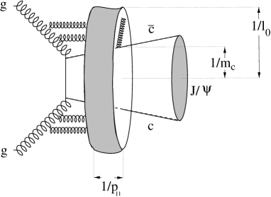
Figure 4: Geometry of the cloud of hard rescattering comovers.

Fig. 4 shows the geometry of the cloud. The majority of all $J/\psi$ are produced at small $p_{\perp}$, so we can think us a situation where the $c\bar{c}$ pair moves essentially in the beam axis. In transversal direction the cloud should have a radius roughly comparable to $1/l_{0}=1/|{\bf\ell}|\sim 1/T$, its longitudinal length however depends on a momentum $p_{\parallel}=\pi/(VT^{2})$. For simplicity we did not take into account this geometry at the ’thermal’ integration $d^{3}{\bf\ell}$ in Eq. (4) etc. $p_{\parallel}$ will grow with $s$. The ratio $x_{\rm cloud}=p_{\parallel}/\sqrt{s}$ which is displayed in Fig. 5, shows what fraction of the energy of the system is transferred to the cloud. Whereas the CTEQ5L gluon distribution leads to a rising fraction (which is rather unphysical), the GRV gluon distribution predicts more or less a constant fraction $x_{\rm cloud}\approx 0.5\%$ for $pA$ collisions and $x_{\rm cloud}\approx 1\%$ for $\pi A$ collisions.

Figure 5: The fraction of energy $x_{\rm cloud}$ transferred from the projectiles to the gluon cloud in $pA$ collisions (right) and $\pi A$ collisions (left).

We are now in a position to predict what cross section we will get with our fit at higher energies and especially with RHIC energies with $\sqrt{s}=200\;{\rm GeV}$.

Figure 6: Total cross section for S-wave charmonium production $\sigma$ in nb versus $\sqrt{s}$: On the left the cross sections for $J/\psi$ production are displayed and on the right the ones for $\psi^{\prime}$ production. The upper two figures show the results for $pA$ and the lower two figures for $\pi A$ collisions. All nuclear effects have been rescaled so that in principle all the cross sections should display the result for $pp$ and $\pi p$ collisions, respectively. The solid and the dashed line show the curves obtained from the combined ($J/\psi$ and $\psi^{\prime}$ data) fit for the temperature depending on which parton distribution has been used.

Fig. 6 shows the fit we made in terms of the total inclusive $J/\psi$ and $\psi^{\prime}$ cross section. The data have been rescaled to use the full range in $x_{F}\in[-1,1]$. For the $\pi A$ collisions we have assumed an $x_{F}$ distribution of the form $d\sigma/dx_{F}\sim(1-|0.18-x_{F}|)^{c}$, with $c=2.5$ for $J/\psi$ and $c=3.9$ for $\psi^{\prime}$ [30]. In case of the $pA$ collisions a symmetric $x_{F}$ distribution is assumed. It turns out that for the latter one the CTEQ5L distribution predicts an unphysical decreasing cross section at large $\sqrt{s}$ therefore we will not consider this distribution in the following any longer, whereas GRV shows in all cases a reasonable relaxing rising behavior. We can now have a more closer look at the details of the various processes contributing using the GRV set only. The first important quantity of interest in the $\chi_{1}/\chi_{2}-{\rm ratio}$. It is defined by:

$$\chi_{1}/\chi_{2}-{\rm ratio}=\frac{\sigma(\chi_{c1}){\rm Br}(\chi_{c1}\to J/\psi)}{\sigma(\chi_{c2}){\rm Br}(\chi_{c2}\to J/\psi)}\;.$$ (42)

A comparison of the data and our results is shown in Tab. 4.

Reference	E beam [GeV]	$(\chi_{1}/\chi_{2})_{\rm exp.}$	$(\chi_{1}/\chi_{2})_{\rm theor.}$
E705 [32]	185	1.4 $\pm$ 0.4	1.0456
E506 [35]	515	1.2 $\pm$ 0.4	0.9194

Table 4: Comparison of the measured $\chi_{1}/\chi_{2}-{\rm ratio}$ in $\pi A$ reaction with the result of the theory described here. For the gluon distribution function the GRV98 $\times$ GRS99 set is used.

It turns out that the values for the $\chi_{1}/\chi_{2}-{\rm ratio}$ are a bit smaller, but well inside the error bars of the measured $\pi A$ reactions. They would be reproduced even better, if we neglected the CSM contributions altogether. In this case we get $(\chi_{1}/\chi_{2})_{\rm theor.}=1.2$ independent of the beam energy, if we set all masses equal to $2m_{c}$. So, in principle the theory is capable to describe the large $\chi_{1}/\chi_{2}-{\rm ratio}$ found experimentally in contrast to the standard COM and CSM theory.

Figure 7: Contribution of various subprocesses to inclusive $J/\psi$ production in $pA$ and $\pi A$ collisions. On the right the ratio of the directly produced $J/\psi$ to all $J/\psi$ measured is displayed. In the middle the ratio between the $\psi^{\prime}$ cross section and the cross section of the directly produced $J/\psi$ is shown. The shape of this ratio changes with $s$ only due to the evolution of the gluon parton density. On the right the ratio $\chi_{c1}/\chi_{c2}$ as discussed in the text is displayed. The underlying gluon distribution for all figures has been taken from GRV and GRS respectively.

Fig. 7 shows some details as to the various subprocesses contributing to the inclusive $J/\psi$ production in $pA$ and $\pi A$ scattering. It is shown that the fraction of directly produced $J/\psi$ versus the whole inclusive cross section decreases with increasing energy until it falls down to about 40% at RHIC energies. The $s$ dependence of the $\sigma(\psi^{\prime})/\sigma(J/\psi)_{\rm dir}$ is governed by the scale dependence of the gluon parton distribution (here GRV) involved. It goes towards a constant for large $s$ which is about 1/4. The $\chi_{c1}/\chi_{c2}$ ratio is rapidly falling with $s$. In all cases the $pA$ and $\pi A$ curves behave similar.

6 Double spin asymmetries

The discussion on the partonic cross section has shown two important consequences:

• As long as we can set the displacement parameter $b$ to zero, which in accordance to the non-polarization of the final $J/\psi$, there is no correlation between the proton spin and the final $J/\psi$ spin orientation. All single spin asymmetries are then zero as to the order of accuracy of the approximations applied here.

• The double spin asymmetries for the directly produced $J/\psi$ and $\psi^{\prime}$ depend up to a factor only on the ratio of the polarized and unpolarized gluon distributions. In case of the inclusive $J/\psi$ cross section the different mass-scales make the situation more complicated.

These findings mean a big simplification for the polarized physics because they state that the extraction of the polarized gluon density from the double spin asymmetry will not be complicated by initial and final state spin correlations. With the model set up in the previous chapter we are able to compute the error bars for the double spin asymmetries for $J/\psi$, $\psi^{\prime}$ and $\chi_{cJ}$ production. In the following we collect the expressions for the double longitudinal spin cross section $\Delta\sigma_{LL}$:

$$\Delta\sigma_{LL} = -\int dx_{1}dx_{2}\sum_{S_{z}}\Sigma_{LL}(S_{z})\quad({\rm general\;formula})$$

$$\Delta\sigma_{LL}(J/\psi)_{\rm dir} = 3\frac{V\zeta(4)}{2\pi^{2}\beta^{4}}\int dx_{1}\int dx_{2}{\cal F}_{S}(M_{J/\psi}^{2})\Delta G(x_{1},M_{J/\psi}^{2})\Delta G(x_{2},M_{J/\psi}^{2})$$

$$\Delta\sigma_{LL}(\psi^{\prime}) = 3\frac{V\zeta(4)}{2\pi^{2}\beta^{4}}\int dx_{1}\int dx_{2}{\cal F}_{S}(M_{\psi^{\prime}{\rm eff}}^{2})\Delta G(x_{1},M_{\psi^{\prime}{\rm eff}}^{2})\Delta G(x_{2},M_{\psi^{\prime}{\rm eff}}^{2})$$

$$\Delta\sigma_{LL}(\chi_{cJ}^{\prime}) = (2J+1)\frac{V\zeta(4)}{2\pi^{2}\beta^{4}}\int dx_{1}\int dx_{2}{\cal F}_{P}(M_{\chi_{cJ}{\rm eff}}^{2})\Delta G(x_{1},M_{\chi_{cJ}{\rm eff}}^{2})\Delta G(x_{2},M_{\chi_{cJ}{\rm eff}}^{2})$$

$$+\Delta\sigma_{LL}^{\rm(CSM)}(\chi_{cJ})$$

$$\Delta\sigma_{LL}(J/\psi)_{\rm incl} = \Delta\sigma_{LL}(J/\psi)_{\rm dir}+{\rm Br}(\psi^{\prime}\to J/\psi)\Delta\sigma_{LL}(\psi^{\prime})+\sum_{J}{\rm Br}(\chi_{cJ}\to J/\psi)\Delta\sigma_{LL}(\chi_{cJ})\;.$$

The - sign in the general formula takes into account that the standard convention for the numerator of the asymmetry is always anti-parallel spin alignment minus parallel spin alignment. For the color singlet (CSM) contributions we find:

$$\Delta\sigma_{LL}^{\rm(CSM)}(\chi_{c0}) = \frac{12\pi^{2}\alpha_{s}^{2}|R_{1}^{\prime}|^{2}}{M_{\chi_{c0}}^{7}}\int dx_{1}dx_{2}\Delta G(x_{1},M_{\chi_{c0}}^{2})\Delta G(x_{2},M_{\chi_{c0}}^{2})\delta\left(1-\frac{M_{\chi_{c}0}^{2}}{Sx_{1}x_{2}}\right)$$

$$\Delta\sigma_{LL}^{\rm(CSM)}(\chi_{c1}) = 0$$

$$\Delta\sigma_{LL}^{\rm(CSM)}(\chi_{c2}) = -\frac{16\pi^{2}\alpha_{s}^{2}|R_{1}^{\prime}|^{2}}{M_{\chi_{c2}}^{7}}\int dx_{1}dx_{2}\Delta G(x_{1},M_{\chi_{c2}}^{2})\Delta G(x_{2},M_{\chi_{c2}}^{2})\delta\left(1-\frac{M_{\chi_{c}2}^{2}}{Sx_{1}x_{2}}\right)\;.$$

The corresponding unpolarized cross sections can be straightforwardly obtained by replacing the polarized by the unpolarized gluon distributions and to remove all minus signs. Then the double spin asymmetry $A_{LL}$ and its statistical error $\delta A_{LL}$ are simply given by:

$$A_{LL}=\delta\sigma_{LL}/\sigma\;;\qquad\delta A_{LL}=2\sqrt{\frac{\sigma_{+}\sigma_{-}}{{\cal L}(\sigma_{+}+\sigma_{-})^{3}}}\;,\quad\sigma_{\pm}=\sigma\pm\Delta\sigma_{LL}\;.$$ (45)

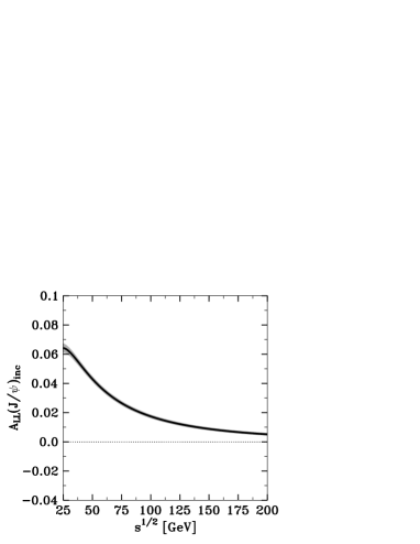
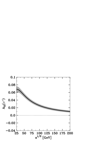
Figure 8: Double spin asymmetry $A_{LL}$ for inclusive $J/\psi$ (left) and $\psi^{\prime}$ (right) hadroproduction. For the plot we use the unpolarized parton distribution set GRV and the polarized GSA. For the grey error band the assumed luminosity is $0.25\;{\rm pb}^{-1}$ using a beam polarization of 100%.

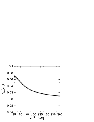
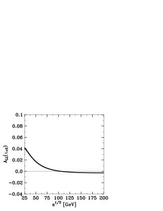
Figure 9: Double spin asymmetry $A_{LL}$ for inclusive $\chi_{cJ},J=0,1,2$ hadroproduction. For the plot we use the unpolarized parton distribution set GRV and the polarized GSA. For the grey error band the assumed luminosity is $0.25\;{\rm pb}^{-1}$ using a beam polarization of 100%.

Fig. 8 shows the double spin asymmetry for S-wave charmonium production, i.e inclusive $J/\psi$ and $\psi^{\prime}$ production. For the polarized gluon distribution amplitude we use the leading order set gluon A [42], which we will abbreviate in the following by GSA. For the error band we have assumed a luminosity of ${\cal L}=0.25\;{\rm pb}^{-1}$. It is seen that for inclusive $J/\psi$ and $\psi^{\prime}$ production the asymmetry at RHIC energies is sizable. It is larger for $\psi^{\prime}$ production, but here also the error bars are larger. For P-wave charmonium production (see Fig. 9) the asymmetry for the $\chi_{c2}$ production is partially negative due to the CSM contribution. In case the CSM contribution is smaller, i.e. that a smaller value for $|R_{1}^{\prime}|$ is more realistic, the asymmetry will go to more positive values, so here we see a very fine test of the interplay between CSM and comovers. In all cases we get a substantial asymmetry for RHIC energies with small error bars. In general it is noticed that the asymmetry decreases with increasing beam energy $\sqrt{s}$. This means that in addition to the RHIC spin program an polarized experiment like HERA-$\vec{N}$, which is supposed to run at $\sqrt{s}=40\;{\rm GeV}$ will also contribute very valuable information for the mechanism how charmonium production happens in hadroproduction. One should notice that the asymmetries for inclusive $J/\psi$ and the $\chi_{c1}$ production do not depend on the temperature while the other asymmetries do, so to measure the asymmetries will give essential new information upon the validity of the theory.

Finally, it has to be stated that the whole calculation still is based on the velocity expansion $p/m$ within the NRQCD formalism, which is truncated already at the first order. The corrections to this may be quite considerable. In this direction we find also the big expansion parameter $\rho$ already determined in [5] and which has been confirmed here. Unfortunately, the inclusion of those velocity corrections will destroy the simple relations derived in [5, 6]. It would be quite advisable for future studies to develop a formalism, that could test the results of the hard comover rescattering from a different stand point which is not based on the approximations of the NRQCD.

7 Summary

In this work we have tried to describe the measured unpolarized cross section for charmonium production through the framework of hard comover rescattering and made predictions for the asymmetries in polarized $pp$ scattering. The generic advantage of the hard comover rescattering mechanism is that it can explain the non-polarization and the comparatively large value for the $\chi_{1}/\chi_{2}$-fraction observed in experiment in a simple and natural way.

In order to get quantitative results we have expressed the comovers as a thermal cloud of gluons. The measured data suggest that about 0.5-1% of the total energy in the collision is invested in the formation of the gluon cloud. The fact, that the final state $J/\psi$ is unpolarized leads us to the conclusion that the displacement parameter $b$ should be small and consistent to zero. If this is true then it means that there is no correlation in polarized experiments between the initial polarization of the protons and the final polarization of the $J/\psi$ and furthermore the single-spin asymmetry $\Sigma_{0L}$ should be zero, a notion which should be tested by experiment. The asymmetries $A_{LL}(\psi^{\prime})$ and $A_{LL}(\chi_{c1})$ depend only on the ratio of the polarized and unpolarized gluon distribution amplitudes, while $A_{LL}(J/\psi)_{\rm incl}$, $A_{LL}(\chi_{c0})$ and $A_{LL}(\chi_{c2})$ are in principle sensitive to the parameters describing the gluon cloud. The hard comover rescattering picture provides an understanding of the formation of onium states in hadroproduction which may give the answers to some problems left unsolved in the standard COM and CSM mechanism. The RHIC-spin experiment and a possible HERA-$\vec{N}$ will provide very crucial new information upon the validity and the consequences of the theory presented here.

Acknowledgments
It is a pleasure to thank Paul Hoyer, Nils Marchal and Stéphane Peigné for fruitful discussion and many explanations concerning their work. I also want to thank Marc Bertini and Torbjorn Sjöstrand for helpful suggestions and ideas.

Appendix A Derivation of the $\chi_{0}$ and $\chi_{2}$ ${\cal O}(\alpha_{s}^{2})$ CSM cross sections

In this appendix we reproduce the Born cross section for $\chi_{0}$ and $\chi_{2}$ production (${\cal O}(\alpha_{s}^{2})$). This gives a cross check for the formulas derived in [5] and also a cross check for the phase-space and flux factors we used in the text to obtain the cross section formulas from the amplitudes.

The momenta for the gluon fusion amplitude are:

$$g_{1}=(m,0,0,m), \quad g_{2}=(m,0,0,-m)$$

$$p_{1}=(m,{\bf p}), \quad p_{2}=(m,-{\bf p})$$ (46)

$$\Phi = -ig^{2}\bar{v}(p_{2},\bar{\lambda})\left[\parbox[b]{6.00006pt}{$\varepsilon$}\parbox[b]{5.50003pt}{ \raisebox{-0.86108pt}{$/$}}_{2}T^{b}\frac{\parbox[b]{6.00006pt}{$p$}\parbox[b]{5.50003pt}{ \raisebox{-0.86108pt}{$/$}}_{1}-\parbox[b]{10.00002pt}{$g$}\parbox[b]{5.50003pt}{ \raisebox{0.86108pt}{$/$}}_{1}+m_{Q}}{(p_{1}-g_{1})^{2}-m_{Q}^{2}}\parbox[b]{6.00006pt}{$\varepsilon$}\parbox[b]{5.50003pt}{ \raisebox{-0.86108pt}{$/$}}_{1}T^{a}+\parbox[b]{6.00006pt}{$\varepsilon$}\parbox[b]{5.50003pt}{ \raisebox{-0.86108pt}{$/$}}_{1}T^{a}\frac{\parbox[b]{6.00006pt}{$p$}\parbox[b]{5.50003pt}{ \raisebox{-0.86108pt}{$/$}}_{1}-\parbox[b]{10.00002pt}{$g$}\parbox[b]{5.50003pt}{ \raisebox{0.86108pt}{$/$}}_{2}+m_{Q}}{(p_{1}-g_{2})^{2}-m_{Q}^{2}}\parbox[b]{6.00006pt}{$\varepsilon$}\parbox[b]{5.50003pt}{ \raisebox{-0.86108pt}{$/$}}_{2}T^{b}\right]u(p_{1},\lambda)$$ (47)

$$+\frac{-g^{2}}{(2m)^{2}}f_{abc}\;{\bf\varepsilon}_{1}\cdot{\bf\varepsilon}_{2}\;\bar{v}(p_{2},\bar{\lambda})(\parbox[b]{10.00002pt}{$g$}\parbox[b]{5.50003pt}{ \raisebox{0.86108pt}{$/$}}_{1}-\parbox[b]{10.00002pt}{$g$}\parbox[b]{5.50003pt}{ \raisebox{0.86108pt}{$/$}}_{2})u(p_{1},\lambda)$$

$$\sim \frac{ig^{2}}{2m}\bar{v}(p_{2},\bar{\lambda})\left[\parbox[b]{6.00006pt}{$\varepsilon$}\parbox[b]{5.50003pt}{ \raisebox{-0.86108pt}{$/$}}_{2}T^{b}(\parbox[b]{6.00006pt}{$p$}\parbox[b]{5.50003pt}{ \raisebox{-0.86108pt}{$/$}}_{1}-\parbox[b]{10.00002pt}{$g$}\parbox[b]{5.50003pt}{ \raisebox{0.86108pt}{$/$}}_{1}+m_{Q})\parbox[b]{6.00006pt}{$\varepsilon$}\parbox[b]{5.50003pt}{ \raisebox{-0.86108pt}{$/$}}_{1}T^{a}\left(\frac{1}{m}+\frac{p_{z}}{m^{2}}\right)\right.$$

$$\qquad\qquad\qquad\left.+\parbox[b]{6.00006pt}{$\varepsilon$}\parbox[b]{5.50003pt}{ \raisebox{-0.86108pt}{$/$}}_{1}T^{a}(\parbox[b]{6.00006pt}{$p$}\parbox[b]{5.50003pt}{ \raisebox{-0.86108pt}{$/$}}_{1}-\parbox[b]{10.00002pt}{$g$}\parbox[b]{5.50003pt}{ \raisebox{0.86108pt}{$/$}}_{2}+m_{Q})\parbox[b]{6.00006pt}{$\varepsilon$}\parbox[b]{5.50003pt}{ \raisebox{-0.86108pt}{$/$}}_{2}T^{b}\left(\frac{1}{m}-\frac{p_{z}}{m^{2}}\right)\right]u(p_{1},\lambda)$$

$$+\frac{g^{2}}{2m}f_{abc}\;{\bf\varepsilon}_{1}\cdot{\bf\varepsilon}_{2}\;\bar{v}(p_{2},\bar{\lambda})\gamma^{3}u(p_{1},\lambda)\;.$$

Using now the equation of motion one can write:

$$\parbox[b]{6.00006pt}{$\varepsilon$}\parbox[b]{5.50003pt}{ \raisebox{-0.86108pt}{$/$}}_{2}T^{b}(\parbox[b]{6.00006pt}{$p$}\parbox[b]{5.50003pt}{ \raisebox{-0.86108pt}{$/$}}_{1}-\parbox[b]{10.00002pt}{$g$}\parbox[b]{5.50003pt}{ \raisebox{0.86108pt}{$/$}}_{1}+m_{Q})\parbox[b]{6.00006pt}{$\varepsilon$}\parbox[b]{5.50003pt}{ \raisebox{-0.86108pt}{$/$}}_{1}T^{a} = -T^{b}T^{a}\left[\parbox[b]{6.00006pt}{$\varepsilon$}\parbox[b]{5.50003pt}{ \raisebox{-0.86108pt}{$/$}}_{1}{\bf\varepsilon}_{2}\cdot{\bf p}+\parbox[b]{6.00006pt}{$\varepsilon$}\parbox[b]{5.50003pt}{ \raisebox{-0.86108pt}{$/$}}_{2}{\bf\varepsilon}_{1}\cdot{\bf p}+m\left({\bf\varepsilon}_{1}\cdot{\bf\varepsilon}_{2}\gamma_{3}+i[{\bf\varepsilon}_{1}\times{\bf\varepsilon}_{2}]^{z}\gamma_{0}\gamma_{5}\right)\right]$$

$$\parbox[b]{6.00006pt}{$\varepsilon$}\parbox[b]{5.50003pt}{ \raisebox{-0.86108pt}{$/$}}_{1}T^{a}(\parbox[b]{6.00006pt}{$p$}\parbox[b]{5.50003pt}{ \raisebox{-0.86108pt}{$/$}}_{1}-\parbox[b]{10.00002pt}{$g$}\parbox[b]{5.50003pt}{ \raisebox{0.86108pt}{$/$}}_{2}+m_{Q})\parbox[b]{6.00006pt}{$\varepsilon$}\parbox[b]{5.50003pt}{ \raisebox{-0.86108pt}{$/$}}_{2}T^{b} = -T^{a}T^{b}\left[\parbox[b]{6.00006pt}{$\varepsilon$}\parbox[b]{5.50003pt}{ \raisebox{-0.86108pt}{$/$}}_{1}{\bf\varepsilon}_{2}\cdot{\bf p}+\parbox[b]{6.00006pt}{$\varepsilon$}\parbox[b]{5.50003pt}{ \raisebox{-0.86108pt}{$/$}}_{2}{\bf\varepsilon}_{1}\cdot{\bf p}-m\left({\bf\varepsilon}_{1}\cdot{\bf\varepsilon}_{2}\gamma_{3}-i[{\bf\varepsilon}_{1}\times{\bf\varepsilon}_{2}]^{z}\gamma_{0}\gamma_{5}\right)\right]\;.$$

The spinor combinations can be expressed as follows:

$$\bar{v}(p_{2},\bar{\lambda})\gamma^{3}u(p_{1},\lambda) = 2m\delta^{-\bar{\lambda}}_{\lambda}2\lambda$$

$$\bar{v}(p_{2},\bar{\lambda})\gamma^{0}\gamma_{5}u(p_{1},\lambda) = 2m\delta^{-\bar{\lambda}}_{\lambda}$$

$$\bar{v}(p_{2},\bar{\lambda})\parbox[b]{6.00006pt}{$\varepsilon$}\parbox[b]{5.50003pt}{ \raisebox{-0.86108pt}{$/$}}u(p_{1},\lambda) = 2m\delta^{\bar{\lambda}}_{\lambda}(-2\lambda)({\bf e}^{*}(2\lambda)\cdot{\bf\varepsilon})\sqrt{2}\;.$$ (49)

Then, using $[T^{a},T^{b}]=if_{abc}T^{c}$ and $\{T^{a},T^{b}\}=d_{abc}T^{c}$, we arrive at the following expression in the first order $p/m$:

$$\Phi = -ig^{2}\left\{i\delta^{-\bar{\lambda}}_{\lambda}[{\bf\varepsilon}_{1}\times{\bf\varepsilon}_{2}]^{z}\left[\left(\frac{1}{N_{c}}\delta_{ab}\delta_{ij}+d_{abc}T^{c}_{ij}\right)-\frac{ip_{z}}{m}f_{abc}T^{c}_{ij}\right]\right.$$ (50)

$$\qquad\left.-2\lambda\delta^{\bar{\lambda}}_{\lambda}\sqrt{2}\left(({\bf e}^{*}(2\lambda)\cdot{\bf\varepsilon}_{1})({\bf\varepsilon}_{2}\cdot{\bf p})+({\bf e}^{*}(2\lambda)\cdot{\bf\varepsilon}_{2})({\bf\varepsilon}_{1}\cdot{\bf p})\right)\frac{1}{m}\left(\frac{1}{N_{c}}\delta_{ab}\delta_{ij}+d_{abc}T^{c}_{ij}\right)\right\}$$

$$\qquad+2\lambda\delta^{-\bar{\lambda}}_{\lambda}{\bf\varepsilon}_{1}\cdot{\bf\varepsilon}_{2}\frac{p_{z}}{m}\left(\frac{1}{N_{c}}\delta_{ab}\delta_{ij}+d_{abc}T^{c}_{ij}\right)\;.$$

Hereby we reproduce up to convention dependent phase factors Eq. (4) in [5]. For the wave function one uses the following expression:

$$\psi_{\lambda\bar{\lambda}}^{L_{z}S_{z}}({\bf q})=\psi_{LL_{z}}\frac{1}{\sqrt{2}}{\bf e}(S_{z})\chi_{-\bar{\lambda}}{\bf\sigma}{\chi}_{\lambda}\;.$$ (51)

Now the amplitude for $\chi_{cJ},J=0,1,2$ production is given by:

$${\cal M}^{(a)}(^{3}P_{J},J_{z})=\sum_{\lambda\bar{\lambda}\atop L_{z}S_{z}}\left(\begin{array}[]{cc}1&1\\ L_{z}&S_{z}\end{array}\right|\left.\begin{array}[]{c}J\\ J_{z}\end{array}\right)\int\frac{d{\bf q}}{(2\pi)^{3}}\phi^{[1]}_{\lambda\bar{\lambda}}({\bf q})\psi_{\lambda\bar{\lambda}}^{L_{z}S_{z}}({\bf q})\;.$$ (52)

With this we find for the $\chi_{c0}$ meson:

$${\cal M}^{(a)}(^{3}P_{0},0)=-g^{2}\frac{1}{N_{c}}\delta_{ij}\delta_{ab}\frac{3}{\sqrt{2\pi m^{3}}}R_{1}^{\prime}\delta_{\lambda_{1}}^{-\lambda_{2}}\;,$$ (53)

with $R_{1}^{\prime}$ being the first derivative of the quarkonium wave function at the origin, as defined by:

$$\int\frac{{\bf q}d^{3}{\bf q}}{(2\pi)^{3}}\psi_{LL_{z}}({\bf q})=i\sqrt{\frac{3}{4\pi m}}R_{1}^{\prime}{\bf e}(L_{z})\;.$$ (54)

Then the partonic cross section is given by:

$$\sigma_{\lambda_{1}\lambda_{2}}(^{3}P_{0},0)_{CSM}=\frac{2\pi}{2(2m)^{4}}\frac{1}{\left(N_{c}^{2}-1\right)^{2}}\sum_{ab}\frac{1}{N_{c}^{2}}\sum_{ij}|{\cal M}^{(a)}(^{3}P_{0},0)|^{2}=\frac{24\pi^{2}\alpha_{s}^{2}|R_{1}|^{2}}{(2m)^{7}}\delta_{\lambda_{1}}^{-\lambda_{2}}\;.$$ (55)

The amplitude for the $\chi_{c1}$ meson vanishes identically. For the $\chi_{c2}$ meson we find then:

$${\cal M}^{(a)}(^{3}P_{2},J_{z})=-g^{2}\frac{2}{N_{c}}\delta_{ij}\delta_{ab}\sqrt{\frac{3}{2\pi m^{3}}}R_{1}^{\prime}\delta_{\lambda_{1}}^{\lambda_{2}}\delta_{J_{z}/2}^{\lambda_{1}}\;,$$ (56)

and we obtain for the partonic cross section henceforward:

$$\sigma^{(a)}_{\lambda_{1}\lambda_{2}}(^{3}P_{2},J_{z})_{\rm CSM}=\frac{32\pi^{2}\alpha_{s}^{2}|R_{1}|^{2}}{(2m)^{7}}\delta_{\lambda_{1}}^{\lambda_{2}}\delta_{J_{z}/2}^{\lambda_{1}}\;.$$ (57)

Appendix B On the alternative of a virtual gluon field $\Gamma$

A virtual gluon field can be parameterized by the transversality condition:

$$\Gamma_{\mu}\Gamma_{\mu^{\prime}}^{*}=g_{\mu\mu^{\prime}}-\frac{l_{\mu}l_{\mu^{\prime}}}{l^{2}}\;.$$ (58)

Taking now the incoming and outgoing charm quark to be on-shell one obtains up to velocity corrections:

$$m_{c}^{2}=(l+p)^{2}=m_{c}^{2}+l^{2}+2p\cdot l\approx l^{2}+2l_{0}m+m_{c}^{2}\;,$$ (59)

which results in:

$$|\Gamma_{0}|^{2}=1+\frac{l_{0}}{2m}\;.$$ (60)

If $|\Gamma_{0}|$ is going to be zero it requires $l_{0}=-2m$ which means that the charm quark gets a negative energy, which is unphysical. Now we can investigate how much the incoming charm quark needs to be off-shell so that we can work with a real gluon field instead:

$$m_{c}^{2}=(l+p)=(1-\epsilon)m_{c}^{2}+2p\cdot l\rightarrow\epsilon\approx\frac{2l_{0}}{m}\;.$$ (61)

Then, for small enough $l_{0}$, we can again treat the off-shellness as a velocity correction along the many others we have neglected in the calculation.

References

- [1] G. P. Ramsey, hep-ph/0001105.
- [2] R. L. Jaffe and D. Kharzeev, Phys. Lett. B455, 306 (1999) [hep-ph/9903280].
- [3] T. Affolder et al. [CDF Collaboration], hep-ex/0004027.
-
[4]
M. Beneke and I. Z. Rothstein,
Phys. Rev. D54, 2005 (1996)
[hep-ph/9603400];
Erratum-ibid. Phys. Rev. D54, 7082 (1996). - [5] P. Hoyer and S. Peigne, Phys. Rev. D59, 034011 (1999) [hep-ph/9806424].
- [6] N. Marchal, S. Peigne and P. Hoyer, hep-ph/0004234.
- [7] G. T. Bodwin, E. Braaten and G. P. Lepage, Phys. Rev. D51, 1125 (1995) [hep-ph/9407339].
- [8] O. Teryaev and A. Tkabladze, Phys. Rev. D56, 7331 (1997) [hep-ph/9612301].
- [9] W. D. Nowak, O. Teryaev and A. Tkabladze, hep-ph/9711290.
- [10] V. A. Korotkov and W. D. Nowak, Nucl. Phys. A622, 78C (1997) [hep-ph/9701371].
- [11] V. A. Korotkov and W. D. Nowak, hep-ph/9908490.
- [12] W. D. Nowak and A. Tkabladze, Phys. Lett. B443, 379 (1998) [hep-ph/9809413].
- [13] E. L. Berger and D. Jones, Phys. Rev. D23, 1521 (1981).
- [14] R. Baier and R. Ruckl, Phys. Lett. B102, 364 (1981).
- [15] T. Morii, S. Tanaka and T. Yamanishi, Phys. Lett. B322, 253 (1994) [hep-ph/9309336].
- [16] F. Yuan and K. Chao, hep-ph/0008302.
- [17] P. Hagler, R. Kirschner, A. Schafer, L. Szymanowski and O. V. Teryaev, hep-ph/0008316.
- [18] F. Yuan and K. Chao, hep-ph/0009224.
- [19] T. Morii, S. Tanaka and T. Yamanishi, Phys. Lett. B372 (1996) 165. [20]
- [20] S. Gupta and P. Mathews, Nucl. Phys. Proc. Suppl. 64, 446 (1998) [hep-ph/9708479].
- [21] S. Gupta, Phys. Rev. D57, 1858 (1998) [hep-ph/9707315].
- [22] S. Gupta and P. Mathews, Phys. Rev. D56, 7341 (1997) [hep-ph/9706541].
- [23] J. Badier et al. [NA3 Collaboration], Z. Phys. C20, 101 (1983).
- [24] C. Biino et al., Phys. Rev. Lett. 58, 2523 (1987).
- [25] C. Akerlof et al., Phys. Rev. D48, 5067 (1993).
- [26] A. Gribushin et al. [E672 and E706 Collaborations], Phys. Rev. D53, 4723 (1996).
- [27] T. Alexopoulos et al. [E-771 Collaboration], Phys. Rev. D55, 3927 (1997).
- [28] J. G. Heinrich et al., Phys. Rev. D44, 1909 (1991).
- [29] R. Baier and R. Ruckl, Z. Phys. C19, 251 (1983).
- [30] G. A. Schuler, “Quarkonium production and decays,” hep-ph/9403387.
- [31] P. Cho and A. K. Leibovich, Phys. Rev. D53, 6203 (1996) [hep-ph/9511315].
- [32] L. Antoniazzi et al. [E705 Collaboration], Phys. Rev. Lett. 70, 383 (1993).
- [33] C. Caso et al., Eur. Phys. J. C3, 1 (1998).
-
[34]
M. H. Schub et al. [E789 Collaboration],
Phys. Rev. D52, 1307 (1995);
Erratum-ibid. Phys. Rev. D53, 570 (1996). - [35] V. Koreshev et al. [E672-E706 Collaborations], Phys. Rev. Lett. 77, 4294 (1996).
- [36] T. Alexopoulos et al. [E771 Collaboration], Phys. Lett. B374, 271 (1996).
- [37] Y. Alexandrov et al. [BEATRICE Collaboration], Nucl. Phys. B557, 3 (1999).
- [38] H. L. Lai et al. [CTEQ Collaboration], Eur. Phys. J. C12, 375 (2000) [hep-ph/9903282].
- [39] M. Gluck, E. Reya and A. Vogt, Eur. Phys. J. C5, 461 (1998) [hep-ph/9806404].
- [40] M. Gluck, E. Reya and I. Schienbein, Eur. Phys. J. C10, 313 (1999) [hep-ph/9903288].
- [41] E. J. Eichten and C. Quigg, Phys. Rev. D52, 1726 (1995) [hep-ph/9503356].
- [42] T. Gehrmann and W. J. Stirling, Phys. Rev. D53, 6100 (1996) [hep-ph/9512406].