Analysis of oscillations of atmospheric neutrinos

Abstract

We briefly review the current status of standard oscillations of atmospheric neutrinos in schemes with two, three, and four flavor mixing. It is shown that, although the pure $\nu_{\mu}\to\nu_{\tau}$ channel provides an excellent $2\nu$ fit to the data, one cannot exclude, at present, the occurrence of additional subleading $\nu_{\mu}\to\nu_{e}$ oscillations ($3\nu$ schemes) or of sizable $\nu_{\mu}\to\nu_{s}$ oscillations ($4\nu$ schemes). It is also shown that the wide dynamical range of energy and pathlength probed by the Super-Kamiokande experiment puts severe constraints on nonstandard explanations of the atmospheric neutrino data, with a few notable exceptions.

1 Introduction

It is well known that the Super-Kamiokande (SK) atmospheric neutrino data can be beautifully explained in terms of $2\nu$ oscillations in the $\nu_{\mu}\to\nu_{\tau}$ channel [1]. This interpretation is also supported by MACRO [2] and by Soudan2 [3]. Conversely, pure $\nu_{\mu}\to\nu_{e}$ oscillations do not provide a good fit to the SK data [4], and are independently excluded by the negative $\nu_{e}$ disappearance searches in the CHOOZ [5] and Palo Verde [6] reactors. Pure $\nu_{\mu}\to\nu_{s}$ oscillations ($\nu_{s}$ being a hypothetical sterile neutrino) are also disfavored by SK [1, 7] (and by MACRO [2]), due to nonobservation of the associated matter effects [8] and neutral current event depletion [9].

Although two-flavor $\nu_{\mu}\to\nu_{\tau}$ oscillations represent the most economical explanation, it should be stressed that, to some extent, additional oscillation channels may be open, as naturally expected in $3\nu$ and $4\nu$ schemes [10] accommodating the current phenomenology. Moreover, $\nu_{\mu}$ disappearance might be driven by dynamics different from the simple mass-mixing mechanism. In this article, we briefly review the status of such solutions, with emphasis on: (i) scenarios involving more than two states ($3\nu$ and $4\nu$ mixing), and (ii) scenarios involving nonstandard dynamics (decay, extra dimensions, decoherence).

2 $3\nu$ oscillations

Assuming that two out of three active $\nu$’s are almost degenerate (say, $m_{1}\simeq m_{2}$), it can be shown [4] that atmospheric $\nu$’s probe only $m^{2}\equiv m^{2}_{3}-m^{2}_{1,2}$ and the mixing matrix elements $U_{\alpha 3}$:

$$3\nu{\rm\ parameter\ space}\;\equiv\;(m^{2},U^{2}_{e3},U^{2}_{\mu 3},U^{2}_{\tau 3})\ ,$$ (1)

with $U^{2}_{e3}+U^{2}_{\mu 3}+U^{2}_{\tau 3}=1$ for unitarity.  

Figure 1: Progress in bounds on $m^{2}$, as derived by $3\nu$ analyses of atmospheric and reactor data, both before and after SK and CHOOZ.

Figure 2: SK zenith distributions, normalized to no-oscillation expectations. Dots with error bars: SK data. Dashed and solid lines: best fits to SK only and to SK+CHOOZ [11].

We present a preliminary update [11] of previous limits [4] on such parameters, using the latest data from SK (70.5 kTy) [1] and CHOOZ [5]. The SK data include 55 zenith bins: 10+10 bins for the subGeV (SG) $e$+$\mu$ events, 10+10 bins for the multiGeV (MG) $e$+$\mu$ events, and 5+10 bins for the upward stopping (US) and through-going (UT) $\mu$ events. For CHOOZ, we use the total rate (one datum). We accurately calculate all such observables, and $\chi^{2}$-fit them (see [4] for details).

Figure 1 shows that the allowed range for $m^{2}$ is stable around $3\times 10^{-3}$ eV². The same figure also shows the impact of SK and CHOOZ in sharpening [11, 4] prior bounds on $m^{2}$ [12].

Figure 2 shows the SK data and the best-fit theoretical distributions. The best fit for SK data only ($\chi^{2}=47.5$, dashed line) is found at

$$(m^{2},\,U^{2}_{e3},\,U^{2}_{\mu 3},\,U^{2}_{\tau 3})\simeq(3.5,\,0.07,\,0.57,\,0.36)\ ,$$ (2)

where $[m^{2}]=10^{-3}$ eV². For $U^{2}_{e3}=0.07$, the theoretical MG$e$ distribution shows a distortion which, however, is well within the uncertainties. The weak preference for $U^{2}_{e3}\neq 0$ is suppressed by CHOOZ data. The SK+CHOOZ best fit ($\chi^{2}=49$, solid lines) basically corresponds to pure $\nu_{\mu}\to\nu_{\tau}$ oscillations with maximal mixing,

$$(m^{2},\,U^{2}_{e3},\,U^{2}_{\mu 3},\,U^{2}_{\tau 3})\simeq(3.0,\,0,\,0.5,\,0.5)\ ,$$ (3)

with limited allowance for extra $\nu_{e}$ mixing [11],

$${\rm SK\ data\ only} : U^{2}_{e3}<0.31\;\;(0.38)\ ,$$ (4)

$${\rm SK+CHOOZ} : U^{2}_{e3}<0.04\;\;(0.07)\ ,$$ (5)

the bounds being at 90 (99%) C.L. for 3 d.o.f. Unfortunately, it appears very difficult to probe (through present atmospheric data) values of $U^{2}_{e3}$ as small as a few %, which may entail interesting Earth matter effects [4, 13]. Constraining $U^{2}_{e3}$ is a major task for future atmospheric [14], reactor [15] and accelerator [16] $\nu$ experiments.

The bounds on $3\nu$ mixing are more evident in the $(\nu_{e},\nu_{\mu},\nu_{\tau})$ triangle plot, embedding the unitarity constraint (see [4, 12] for details). Figure 3 shows the allowed regions in such triangle, whose lower and right sides represent the subcases of pure $\nu_{\mu}\to\nu_{\tau}$ (allowed) and pure $\nu_{\mu}\to\nu_{e}$ (excluded). Large $\nu_{e}$ mixing is allowed by SK alone, but not by the SK+CHOOZ combination, where only a narrow region survives near the lower side of the triangle. In such region, $U^{2}_{\mu 3}\sim U^{2}_{\tau 3}$ within a factor of two [e.g., $(U^{2}_{\mu 3},\,U^{2}_{\tau 3})\simeq(2/3,\,1/3)$ is also allowed]. In conclusion, the $3\nu$ analysis of SK+CHOOZ shows that the $\nu_{\mu}\to\nu_{e}$ channel might be open with a few $\%$ amplitude. Future atmospheric, reactor, and accelerator $\nu$ experiments will test this interesting possibility.

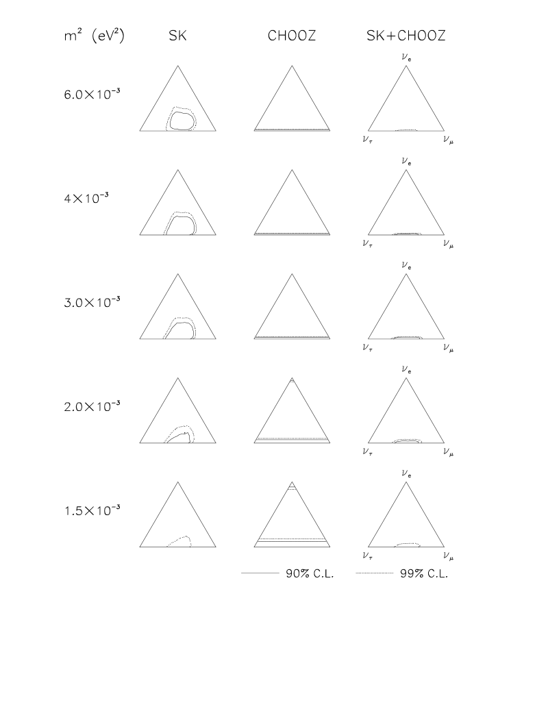
Figure 3: Three-flavor analysis in the $(\nu_{e},\nu_{\mu},\nu_{\tau})$ triangle plot, for five representative values of $m^{2}$. Left and middle column: separate analyses of Super-Kamiokande 70.5 kTy data and CHOOZ final data, respectively. Right column: combined SK+CHOOZ allowed regions. The SK+CHOOZ solutions are close to pure $\nu_{\mu}\leftrightarrow\nu_{\tau}$ oscillations, with upper limits on $U^{2}_{e3}$ in the few percent range [11].

3 $4\nu$ oscillations

The current evidence for $\nu$ oscillations coming from solar, atmospheric, and LSND data can be accommodated by introducing a fourth, sterile neutrino state $\nu_{s}$ [10]. The mass spectrum seems then to be favored in the “2+2” form (two separated doublets) [17], although the “3+1” option (triplet plus singlet) is not dismissed [18].

In 2+2 models, it is often assumed that atmospheric $\nu$ oscillations involve either the $\nu_{\mu}\to\nu_{\tau}$ or the $\nu_{\mu}\to\nu_{s}$ channel. Correspondingly, it is assumed that solar $\nu$ oscillations involve either the $\nu_{e}\to\nu_{s}$ or the $\nu_{e}\to\nu_{\tau}$ channel. Such simplifying assumptions are challenged by the most recent SK data [1, 19], which disfavor oscillations into $\nu_{s}$ for both atmospheric and solar neutrinos. However, it should be realized that atmospheric $\nu_{\mu}$’s and solar $\nu_{e}$’s may also oscillate into linear combinations of $\nu_{s}$ and $\nu_{\tau}$ [20] (rather than into $\nu_{s}$ and $\nu_{\tau}$ separately), e.g.,

$${\rm atm.\ neutrino\ oscillations} : \nu_{\mu}\to\nu_{+}\ ,$$ (6)

$${\rm solar\ neutrino\ oscillations} : \nu_{e}\to\nu_{-}\ ,$$ (7)

where

$$\left(\begin{array}[]{c}\nu_{+}\\ \nu_{-}\end{array}\right)=\left(\begin{array}[]{cc}+\cos\xi&+\sin\xi\\ -\sin\xi&+\cos\xi\\ \end{array}\right)\left(\begin{array}[]{c}\nu_{\tau}\\ \nu_{s}\end{array}\right)\ ,$$ (8)

with $\xi$ to be constrained by experiments. A recent analysis of $\nu_{e}\to\nu_{-}$ solar oscillations shows that all the usual solutions (MSW or vacuum) are compatible with solar data for $\sin^{2}\xi>0.3$ [21].

Concerning atmospheric $\nu$’s, we have analyzed [22] the same data as in Fig. 2 for $\xi\in[0,\pi/2]$. Figure 4 shows some representative results of the $\chi^{2}$ fit, as a function of the mass square difference $m^{2}$. The fit for unconstrained $\xi$ (thick solid line) is almost equal to the one for $\xi=0$ (pure $\nu_{\mu}\to\nu_{\tau}$, thin solid line), implying that the SK data prefer small or zero admixture of $\nu_{s}$. The case $\xi=\pi/2$ (pure $\nu_{\mu}\to\nu_{s}$, dashed line) leads to $\Delta\chi^{2}\simeq 15$ and is disfavored. However, the case $\xi=\pi/4$ (fifty-fifty admixture of $\nu_{\tau}$ and $\nu_{s}$, dotted line) leads only to a modest increase in $\chi^{2}$ and cannot be excluded.

The $4\nu$ analysis can also be done in a triangle plot (different from the $3\nu$ case) embedding the $(\nu_{\mu},\nu_{s},\nu_{\tau})$ unitarity constraint [22]. Figure 5 shows the results for separate and combined SK data sets. It can be seen that, in the combination, the case of pure $\nu_{\mu}\to\nu_{\tau}$ oscillations (left side) is allowed, while the case of pure $\nu_{\mu}\to\nu_{s}$ oscillations (right side) is significantly disfavored. However, there are intermediate solutions for $\sin^{2}\xi<0.7$ which have a significant admixture of $\nu_{s}$. Such results and constraints emerge from the interplay of low-energy data (which are more sensitive to $m^{2}$) and high-energy data (more sensitive to the $\nu_{s}$ component through matter effects, scaling as $\frac{1}{2}$ neutron density $\times\sin^{2}\xi$ [22]).

Figure 4: $\chi^{2}$ fit of 55 SK data bins (70.5 kTy) for $\nu_{\mu}\to\nu_{+}$ oscillations, under various assumptions for the $\nu_{s}$ component of $\nu_{+}$. A large $\nu_{s}$ component (e.g., 50%, dotted line) is not excluded [22].

A qualitative comparison between such results [22] and those in [21] indicates that atmospheric $\nu$ data can be reconciled with any of the oscillation solutions to the solar $\nu$ problem in the range $0.3<\sin^{2}\xi<0.7$. A somewhat different $4\nu$ analysis [23] derives similar conclusions. Summarizing, it turns out that world $\nu$ oscillation data are consistent with $4\nu$ solutions to the solar and atmospheric anomalies, involving oscillations into both active and sterile states at the same time.

Figure 5: $4\nu$ analysis in the $(\nu_{\mu},\nu_{s},\nu_{\tau})$ triangle plot, for five representative values of $m^{2}$. First three columns: separate analyses of SG$e$+SG$\mu$, MG$e$+MG$\mu$, and US$\mu$+UT$\mu$ data. Right column: all SK data (70.5 kTy). The allowed regions typically include pure $\nu_{\mu}\leftrightarrow\nu_{\tau}$ oscillations (left side of the triangle) and disfavor pure $\nu_{\mu}\to\nu_{s}$ oscillations (right side of the triangle). However, intermediate situations with $\nu_{\mu}$ mixing with both $\nu_{\tau}$ and $\nu_{s}$ are allowed inside the triangle [22].

4 Nonstandard dynamics

The SK data probe three decades in pathlength $L$ and four decades in energy $E$. Such a wide dynamical range severely constrains deviations from the standard $L/E$ behavior of the $P_{\mu\tau}$ transition probability, which are expected in the presence of exotic dynamics [24] (e.g., violations of relativity principles [25, 26], which lead to a $L\cdot E$ behavior).

An analysis of older data (45 kTy) has shown that, assuming a $L\cdot E^{n}$ dependence of the phase, the SK measurements constrain $n$ to be very close to $-1$, thus favoring standard oscillations, and excluding several nonstandard explanations [27]. Such results, shown in Fig. 6, have been strengthened by the latest SK data [1]. A peculiar FCNC scenario with $n=0$ [28] is also strongly disfavored—as any energy independent mechanism for $\nu_{\mu}$ disappearance—by combining low and high energy SK data [29]. Therefore, $P_{\mu\tau}$ seems to be (dominantly) a function of $L/E$.

However, is $P_{\mu\tau}$ necessarily a periodic function of $L/E$? The answer is, surprisingly, no. There are (at least) three exotic scenarios which predict a monotonic decrease of the oscillation probability in the relevant $L/E$ range, and that are anyway reasonably consistent with the data.

Figure 6: Bounds on the energy exponent $n$, assuming oscillation phase $\propto L\cdot E^{n}$. (Older 45 kTy SK data used in this figure [27].)

The first scenario involves $\nu$ decay [30], with a decay length of the order of the Earth radius. The second scenario [31] assumes $\nu_{\mu}$ mixing with neutrino states propagating in large extra dimensions [32]. A third scenario [33] assumes nonstandard Liouville dynamics [34], leading to $\nu$ decoherence and thus to a damping of oscillations. Figure 7 shows that the best fit for pure decoherence does not differ significantly from the standard oscillation one [33]. The two cases shown in Fig. 7 correspond to different functional forms for $P_{\mu\mu}$,

$${\rm oscillation:\ }P_{\mu\mu} \simeq \textstyle\frac{1}{2}[1+\cos(+\rho L/E)]\ ,$$ (9)

$${\rm decohere.:\ }P_{\mu\mu} \simeq \textstyle\frac{1}{2}[1+\exp(-\rho L/E)]\ ,$$ (10)

with $[E]=$ GeV, $[L]=$ km, and $\rho\simeq 7\times 10^{-3}$ GeV/km in both cases. Such forms have the same asymptotic behavior, namely, $\langle P_{\mu\mu}\rangle\simeq 1(\frac{1}{2})$ for small (large) $L/E$, but they significantly differ for intermediate values of $L/E$ where, however, the large energy-angle smearing of SK prevents a clear discrimination.

Although such nonstandard explanations [30, 31, 33] of SK data do not survive Occam’s razor, they survive the current experimental tests for a simple reason: the oscillation pattern (appearance of $\nu_{\tau}$ and re-appearance of $\nu_{\mu}$) has not been directly observed so far, and a monotonic $\nu_{\mu}$ disappearance is not excluded yet. Therefore, the unambigous observation of an oscillation cycle represents an important task for future atmospheric [14] and accelerator [16] $\nu$ experiments.

Figure 7: Comparison of standard oscillations (solid line) vs neutrino decoherence (dashed line) as explanation of the SK data. See [33] for details.

5 Conclusions

Two-flavor $\nu_{\mu}\to\nu_{\tau}$ oscillations represent a simple and beautiful explanation of the SK data (as well as of MACRO and Soudan2). However one cannot exclude, in addition, subleading $\nu_{\mu}\to\nu_{e}$ transitions (possible in $3\nu$ models) or sizable $\nu_{\mu}\to\nu_{s}$ transitions (possible in $4\nu$ models). Moreover, the nonobservation of an oscillation cycle still leaves room for exotic dynamics. Further experimental and theoretical work is needed to firmly establish both the flavors and the dynamics involved in atmospheric $\nu_{\mu}$ disappearance.

References

- [1] H. Sobel, these Proceedings.
- [2] B. Barish, these Proceedings.
- [3] T. Mann, these Proceedings.
- [4] G.L. Fogli, E. Lisi, A. Marrone, and G. Scioscia, Phys. Rev. D 59, 033001 (1999).
- [5] CHOOZ coll., Phys. Lett. B 466, 415 (1999).
- [6] G. Gratta, these Proceedings.
- [7] SK collaboration, hep-ex/0009001.
- [8] E. Akhmedov, P. Lipari, and M. Lusignoli, Phys. Lett. B 300, 128 (1993); P. Lipari and M. Lusignoli, Phys. Rev. D 58, 073005 (1998); Q.Y. Liu and A.Yu. Smirnov, Nucl. Phys. B 524, 505 (1998); Q.Y. Liu, S.P. Mikheyev, and A.Yu. Smirnov, Phys. Lett. B 440, 319 (1998); N. Fornengo, M.C. Gonzalez-Garcia, and J.W.F. Valle, Nucl. Phys. B 580, 58 (2000).
- [9] F. Vissani and A.Yu. Smirnov, Phys. Lett. B 432, 376 (1998); L.J. Hall and H. Murayama, Phys. Lett. B 436, 323 (1998).
- [10] See talks by B. Kayser, R. Mohapatra, and A.Yu. Smirnov, these Proceedings.
- [11] G.L. Fogli, E. Lisi, and A. Marrone, work in progress.
- [12] G.L. Fogli, E. Lisi, D. Montanino, and G. Scioscia, Phys. Rev. D 55, 4385 (1997).
- [13] S.T. Petcov, Phys. Lett. B 434, 321 (1998); E. K. Akhmedov, A. Dighe, P. Lipari, and A.Yu. Smirnov, Nucl. Phys. B 542, 3 (1999); J. Pantaleone, Phys. Rev. Lett. 81, 5060 (1998); G.L. Fogli, E. Lisi, A. Marrone, and D. Montanino, Phys. Lett. B 425, 341 (1998); A. De Rujula, M.B. Gavela, and P. Hernandez, hep-ph/0001124.
- [14] A. Geiser, these Proceedings.
- [15] L. Mikaelyan, these Proceedings.
- [16] See talks by A. De Rujula, K. Nakamura, A. Rubbia, and S. Wojcicki, these Proceedings.
- [17] S.M. Bilenky, C. Giunti, and W. Grimus, in Neutrino ’96 (World Scientific, 1997), p.174; V. Barger, S. Pakvasa, T.J. Weiler, and K. Whisnant, Phys. Rev. D 58, 093016 (1998).
- [18] V. Barger, B. Kayser, J. Learned, T. Weiler, and K. Whisnant, hep-ph/0008019.
- [19] Y. Suzuki, these Proceedings.
- [20] See, e.g., D. Dooling, C. Giunti, K. Kang, and C.W. Kim, Phys. Rev. D 61, 073011.
- [21] C. Giunti, M.C. Gonzalez-Garcia, and C. Peña-Garay, Phys. Rev. D 62, 013005 (2000); M.C. Gonzalez-Garcia, these Proceedings.
- [22] G.L. Fogli, E. Lisi, and A. Marrone, “Four neutrino oscillation solutions of the atmospheric neutrino anomaly”, to appear.
- [23] O. Yasuda, hep-ph/0006319.
- [24] P. Lipari and M. Lusignoli, Phys. Rev. D 60, 013003 (1999); G.L. Fogli, E. Lisi, A. Marrone, and G. Scioscia, Phys. Rev. D 59, 117303 (1999).
- [25] M. Gasperini, Phys. Rev. D 38, 2635 (1988).
- [26] S. Coleman and S.L. Glashow, Phys. Lett. B 405, 249 (1997); S.L. Glashow, A. Halprin, P.I. Krastev, C.N. Leung, and J. Pantaleone, Phys. Rev. D 56, 2433, 1997.
- [27] G.L. Fogli, E. Lisi, A. Marrone, and G. Scioscia, Phys. Rev. D 60, 053006 (1999).
- [28] M.C. Gonzalez-Garcia et al., Phys. Rev. Lett. 82, 3202 (1999).
- [29] M.M. Guzzo, H. Nunokawa, O.L.G. Peres, and R. Zukanovich Funchal, Nucl. Phys. B (Proc. Suppl.)) 87, 201 (2000).
- [30] V. Barger, J.G. Learned, P. Lipari, M. Lusignoli, S. Pakvasa, and T.J. Weiler, Phys. Lett. B 462, 109 (1999).
- [31] R. Barbieri, P. Creminelli, and A. Strumia, hep-ph/0002199.
- [32] K. Dienes, these Proceedings.
- [33] E. Lisi, A. Marrone, and D. Montanino, Phys. Rev. Lett. 85, 1166 (2000).
- [34] F. Benatti and R. Floreanini, JHEP 2, 32 (2000).