Skyrmion-anti-Skyrmion Annihilation with $\omega$ Mesons

We study numerically the annihilation of an $\omega$-stabilized Skyrmion and an anti-Skyrmion in three spatial dimensions. To our knowledge this is a first successful simulation of Skyrmion-anti-Skyrmion annihilation which follows through to the point where the energy is carried by outgoing meson waves.

We encounter instabilities similar to those encountered is earlier calculations, but in our case these are not fatal and we are able to simulate through this process with a global energy loss of less than $8\%$, and to identify robust features of the final radiation pattern. The system passes through a singular configuration at the time of half-annihilation. This is followed by the onset of fast oscillations which are superimposed on the smoother process which leads to the appearence of outgoing spherical waves.

We investigate the two prominent features of this process, the proliferation of small, fast oscillations, and the singular intermediate configuration. We find that our equations of motion allow for a regime in which the amplitude of certain small perturbations increases exponentially. This regime is similar but not identical to the situation pointed out earlier regarding the original Skyrme model. We argue that the singularity may be seen as the result of a pinch effect similar to that encountered in plasmas.

1 Introduction

The attractive idea of representing nucleons as solitons of the effective pion field was proposed by Skyrme long before the advent of QCD [1]. In the context of QCD, the idea remains equally attractive, moreover the approach becomes exact in the large $N_{c}$ limit [2]. The Skyrme approach gives a classical, nonperturbative picture of hadrons in the context of low energy QCD. Many properties of nucleons are reobtained using a model of quantized spinning solitons of the pion field [3], including the static nucleon-nucleon and nucleon-antinucleon [4] potential.

The main difficulty in using the Skyrme approach as a starting point for an effective dynamical theory of nucleons lies in the fact that all such enterprises must use numerical calculations to describe the dynamics of the solitons. No analytic solutions are known. One path is to study the classical dynamics of Skyrmions and use the results to build up the quantum dynamics of nucleons based on the model of the static nucleon as a superposition of spinning Skyrmions. Conceptually the simplest process one might study this way is low-energy nucleon-antinucleon annihilation since in this case there are no nucleons in the final state. At low energies the initial state is reasonably well described by Skyrmions, while in the final state there are only mesons which again are well described by the effective theory [5].

Simulating soliton-antisoliton annihilation has proven to be a difficult numerical problem. Previous attempts to simulate the annihilation of a Skyrmion-anti-Skyrmion pair [6, 7, 8] using the original Skyrme Lagrangian encountered numerical difficulties. The problem has been [6] traced to a deviation from the hyperbolic nature of the equations of motion, resulting from the contact nature of the Skyrme term. Another possible concern is that the low-energy approximation becomes questionable during the annihilation process when the energy tied up in the solitons is suddenly liberated. Notwithstanding, below we present a first successful attempt at such a simulation using omega stabilization instead of the Skyrme term. We are able to follow the Skyrmions from incidence through annihilation to pion radiation. An interesting phenomenon involving a possible pointlike singularity arises in our calculation that might actually simplify the analysis, however, our objective for now is to obtain a baseline calculation using classical Skyrmion dynamics. We will return to a detailed dicussion of the singularities in a subsequent publication.

In this paper we present our results on Skyrmion-anti-Skyrmion annihilation using a model [9, 10] which couples a $U(1)$ vector field (the $\omega$) to the winding number of the $SU(2)$ (pion) field. This coupling replaces the Skyrme term for stabilizing the Skyrmion. The omega stabilization is gentler than the Skyrme term and should thus lead to less violent behavior in the simulations. We are able to follow through the annihilation process to the point when the energy is carried by outgoing spherical (pion and $\omega$) waves. We encountered significant, but not fatal, numerical difficulties, and could ensure energy conservation to better than $8\%$ . Our programs are set up for general initial conditions, and we will investigate dependence on those separately. The results we present below refer only to the head-on annihilation process with fixed initial velocity. To our knowledge the annihilation process has not been followed this far previously.

The annihilation itself, in the sense of the unwinding of the baryon number, takes place in a time comparable to the size of the Skyrmions. It proceeds through an intermediary state which has a pointlike singularity, which results in the concentration of the total energy in a very small region around the symmetry center. This is followed by fast oscillations which last for a time comparable to the unwinding, and then gradually give way to outgoing (quasi)spherical waves.

For the original Skyrme model, the Skyrme term was identified as the source of numerical instability [6]. Our effective Lagrangian does not have a similar local self-interaction term for the pion field. However, we have encountered numerical problems similar to those expected when the equations are no longer purely hyperbolic, namely, the appearence of persistent fast oscillations of small amplitude which make the simulation difficult. After a more careful analysis, we found that our equations of motion also allow for non-hyperbolic solutions, (i.e., plane waves with imaginary wave number) albeit at a higher order than the Skyrme equations. Fortunately, in our case these oscillations are weak enough as to not completely destroy the long-wavelength features. Thus our central results seem to be robust and independent of the violent short wave length behavior.

The most prominent feature of the annihilation process, and probably the ultimate source of our numerical difficulties, is the fact that close to the point of half-annihilation, when the original tips of the Skyrmion and the anti-Skyrmion merge, the pion field has a singular configuration. The fields themselves are continuous, but the derivatives are singular. We do not yet have a complete, quantitative understanding of this phenomenon, but it is clear that it consists of the axial baryon current (which carries out the annihilation) being squeezed into a very small, probably pointlike cross-section. This feature is localized in the $x=0$ symmetry plane (the one that separates the Skyrmion and the anti-Skyrmion), and arises close to the moment of half-annihilation.

In the following section we define our model Lagrangian and derive the equations of motion. The main part of this paper is contained in Sec.3, where we describe our numerical results on the phenomenology of axial-symmetric annihilation and discuss our simulation. The first part of this section describes our calculation, with emphasis on aspects not already discussed in [9]. The reader interested only in the phenomenology of the annihilation may skip directly to Sec.3.2, and omit Sec.3.3 where we present numerical checks to assess the reliability of our results. In Section 4 we investigate the stability of our equations of motion against small plane-wave like perturbations, in the spirit of [6], and attempt to identify signs of non-hyperbolicity in our results. In Section 5 we discuss the appearence of a singularity in the pion field at the moment of half-annihilation. While we can understand qualitatively the mechanism that produces this phenomenon, a full understanding will require more focused investigation. Finally in Sec.6 we summarize our results and make a wish list of further work.

2 The model

Our Lagrangian consists of the nonlinear sigma model piece

$${\cal L}_{\sigma}~{}=~{}\frac{1}{4}f_{\pi}^{2}{\mathrm{t}r}\left(\partial_{\mu}{\cal U}\partial^{\mu}{\cal U}^{\dagger}\right)+\frac{1}{2}m_{\pi}^{2}f_{\pi}^{2}{\mathrm{t}r}\left({\cal U}-1\right)~{}~{}$$ (1)

and the omega piece,

$${\cal L}_{\omega}~{}=~{}-\frac{1}{2}\partial_{\mu}\omega_{\nu}(\partial^{\mu}\omega^{\nu}-\partial^{\nu}\omega^{\mu})+\frac{1}{2}M^{2}\omega_{\mu}\omega^{\mu}$$ (2)

which are coupled through the baryon current,

$${\cal L}_{int}~{}=~{}\frac{3g}{2}\omega_{\mu}B^{\mu}~{}~{}~{};~{}~{}~{}B^{\mu}~{}=~{}\frac{1}{12\pi^{2}}\epsilon^{\mu\nu\alpha\beta}{\mathrm{t}r}\left(\left({\cal U}^{\dagger}\partial_{\nu}{\cal U}\right)\left({\cal U}^{\dagger}\partial_{\alpha}{\cal U}\right)\left({\cal U}^{\dagger}\partial_{\beta}{\cal U}\right)\right)~{}~{}~{}.$$ (3)

The $SU(2)$ field ${\cal U}$ is parameterized by the three real pion fields $\{\pi_{k}\}_{k=1,3}=\vec{\pi}$, or by the four ’Cartesian’ components ${\bf\Psi}=\{\Psi^{A}\}_{A=0,3}$,

$${\cal U}~{}=\exp\left(i\vec{\tau}\cdot\vec{\pi}\right)~{}=~{}\Psi_{0}~{}+~{}i\vec{\tau}\cdot\vec{\Psi}~{}=~{}S^{A}\Psi^{A}~{}~{}~{}~{}(A=0,\ldots,3)~{}~{}~{}.$$ (4)

In our previous calculation we have used the $\pi$ parameterization exclusively. For a detailed derivation of the equations of motion and a description of the corresponding numerical method we refer the reader to [9]. The more traditional method is to use the $\Psi$ parameterization. That choice of variables has the advantage of being more transparent. Below we derive the equations of motion in the $\Psi$ parameterization, and describe a way to employ them in simulations without having to deal with Lagrange multipliers as dynamical vairables. We used this approach to perform numerical calculations together with another code based on the $\pi$ parameterization. The equations of motion below are crucial for the analysis presented in Section 4.

In the $\Psi$ parameterization the baryon current is

$$B^{\mu}~{}=~{}\frac{1}{12\pi^{2}}\epsilon^{\mu\nu\alpha\beta}\epsilon^{ABCD}\Psi^{A}\partial_{\nu}\Psi^{B}\partial_{\alpha}\Psi^{C}\partial_{\beta}\Psi^{D}~{}~{},$$ (5)

and the nonlinear $\sigma$ piece is given by

$${\cal L}_{\sigma}~{}=~{}\frac{1}{2}f_{\pi}^{2}\partial_{\mu}\Psi^{A}\partial^{\mu}\Psi^{A}+\frac{1}{2}m_{\pi}^{2}f_{\pi}^{2}\left(\Psi^{0}-1\right)~{}~{}.$$ (6)

The $\Psi^{A}$’s are subject to the chiral constraint which is equivalent to the unitarity condition on the $\cal U$’s:

$${\cal U}{\cal U}^{\dagger}~{}=~{}{\bf 1}~{}~{}~{}\rightarrow~{}~{}~{}\Psi^{A}\Psi^{A}~{}=~{}1~{}~{}~{}.$$ (7)

To get meaningful equations of motion, we must impose this constraint separately on the components $\Psi^{A}$. One way is to introduce a Lagrange multiplier $\lambda$, adding a term $\frac{\lambda}{2}\left(\Psi^{A}\Psi^{A}-1\right)$ to the Lagrangian. The physical meaning of the multiplier is similar to that of ’reaction’ forces in mechanics, which enforce constraints without performing any work. Obviously, the equation of motion for $\lambda$ is just the constraint equation (7), which now has to be solved along with the other equations of motion.

Our task is to solve formally the ordinary equations of motion for the dynamical variables and their derivatives. These will contain $\lambda$. Then, one uses the result and the constraint equation to solve for $\lambda$. Below, this will turn out to be straightforward.

To obtain the equations of motion for $\Psi^{A}$, start with the derivatives of ${\cal L}_{\sigma}~{}+~{}{\cal L}_{\lambda}$:

$$\frac{\delta({\cal L}_{\sigma}+{\cal L}_{\lambda})}{\delta(\Psi^{A})}~{}=~{}m_{\pi}^{2}f_{\pi}^{2}\delta^{A0}\Psi^{0}~{}+~{}\lambda\Psi^{A}~{}~{};~{}~{}\frac{\delta({\cal L}_{\sigma}+{\cal L}_{\lambda})}{\delta(\partial_{\mu}\Psi^{A})}~{}=~{}f_{\pi}^{2}\partial^{\mu}\Psi^{A}~{}~{};~{}~{}\partial_{\mu}\frac{\delta({\cal L}_{\sigma}+{\cal L}_{\lambda})}{\delta(\partial_{\mu}\Psi^{A})}~{}=~{}f_{\pi}^{2}\partial_{\mu}\partial^{\mu}\Psi^{A}~{}~{}.$$

The derivatives of ${\cal L}_{int}$ are:

$$\frac{\delta{\cal L}_{int}}{\delta(\Psi^{A})}~{} = ~{}\frac{g}{8\pi^{2}}\epsilon^{\mu\nu\alpha\beta}\omega_{\mu}\epsilon^{ABCD}\partial_{\nu}\Psi^{B}\partial_{\alpha}\Psi^{C}\partial_{\beta}\Psi^{D}$$

$$\partial_{\nu}\frac{\delta{\cal L}_{int}}{\delta(\partial_{\nu}\Psi^{B})}~{} = ~{}\frac{3g}{8\pi^{2}}\left\{\epsilon^{\mu\nu\alpha\beta}\omega_{\mu}\epsilon^{ABCD}\partial_{\nu}\Psi^{A}\partial_{\alpha}\Psi^{C}\partial_{\beta}\Psi^{D}~{}+~{}\epsilon^{\mu\nu\alpha\beta}\partial_{\nu}\omega_{\mu}\epsilon^{ABCD}\Psi^{A}\partial_{\alpha}\Psi^{C}\partial_{\beta}\Psi^{D}~{}\right\}~{}.$$

The $\Psi^{A}$ equation of motion is:

$$f_{\pi}^{2}\partial_{\mu}\partial^{\mu}\Psi^{A}~{} = ~{}\frac{3g}{8\pi^{2}}\epsilon^{\alpha\beta\mu\nu}\epsilon^{ABCD}\left\{\partial_{\nu}\omega_{\mu}\Psi^{B}\partial_{\alpha}\Psi^{C}\partial_{\beta}\Psi^{D}~{}+~{}\frac{4}{3}\omega_{\mu}\partial_{\nu}\Psi^{B}\partial_{\alpha}\Psi^{C}\partial_{\beta}\Psi^{D}\right\}~{}+~{}$$ (8)

$$~{}~{}~{}+~{}m_{\pi}^{2}f_{\pi}^{2}\delta^{A0}\Psi^{0}~{}+~{}\lambda\Psi^{A}~{}~{}.$$

We can now proceed to eliminating $\lambda$. The chiral condition means that ${\bf\Psi}=\left\{\Psi^{A}\right\}$ is a four-dimensional unit vector. This leads to constraints of its derivatives. The first derivative of $\bf{\Psi}$ with respect to any one of the four cordinates must be perpendicular to $\bf{\Psi}$, and so on:

$$\Psi^{A}\Psi^{A}~{}=~{}1~{}~{}\rightarrow~{}~{}\partial_{\mu}\Psi^{A}\Psi^{A}~{}=~{}0~{}~{}\rightarrow~{}~{}\sum\limits_{A}\left(\partial^{2}_{\mu}\Psi^{A}\right)\Psi^{A}+\sum\limits_{A}\left(\partial\Psi^{A}\right)^{2}~{}=~{}0~{}~{},$$

or, after summing over $\mu$:

$$\partial_{\mu}\partial^{\mu}\Psi^{A}\Psi^{A}~{}+~{}\partial_{\mu}\Psi^{A}\partial^{\mu}\Psi^{A}~{}=~{}0~{}~{}.$$ (9)

Geometrically this means that the component of $\partial_{\mu}\partial^{\mu}\bf{\Psi}$ parallel to $\bf{\Psi}$ is not a dynamical variable, but rather it is determined by the constraint. The corresponding part of the equation of motion (8) therefore carries no information about $\bf{\Psi}$. Instead, it tells us what $\lambda$ should be in order to make sure (9) and thus (7) are verified.

Now we just project (8) onto $\bf{\Psi}$ and solve for $\lambda$:

$$\lambda~{} = ~{}f_{\pi}^{2}\Psi^{A}\partial_{\mu}\partial^{\mu}\Psi^{A}~{}-~{}\frac{g}{2\pi^{2}}\epsilon^{\mu\nu\alpha\beta}\epsilon^{ABCD}\omega_{\mu}\Psi^{A}\partial_{\nu}\Psi^{B}\partial_{\alpha}\Psi^{C}\partial_{\alpha}\Psi^{D}~{}-~{}m_{\pi}^{2}f_{\pi}^{2}(\Psi^{0})^{2}$$ (10)

$$= ~{}-~{}f_{\pi}^{2}\partial_{\mu}\Psi^{A}\partial^{\mu}\Psi^{A}~{}-~{}\frac{g}{2\pi^{2}}\epsilon^{\mu\nu\alpha\beta}\epsilon^{ABCD}\omega_{\mu}\Psi^{A}\partial_{\nu}\Psi^{B}\partial_{\alpha}\Psi^{C}\partial_{\alpha}\Psi^{D}~{}-~{}m_{\pi}^{2}f_{\pi}^{2}(\Psi^{0})^{2}~{}~{}.$$

From the second form it is clear that we have indeed solved for $\lambda$. Remember that we have a set of second-order partial differential equations. An initial condition specifies all the fields and their first derivatives, so the right-hand side of the second equation contains only known quatities. We can now replace this expression for $\lambda$ into the full equation of motion.

One more observation is necessary. Since ${\bf\Psi}$ is a unit vector, all the $\partial_{\mu}{\bf\Psi}$’s are perpendicular to it. Consider the quantity

$$\epsilon^{\mu\nu\alpha\beta}\epsilon^{ABCD}\partial_{\nu}\Psi^{B}\partial_{\alpha}\Psi^{C}\partial_{\beta}\Psi^{D}~{}~{}.$$ (11)

Each nonzero term in the sum over Lorentz indices is perpendicular (in isospin space) to three distinct vectors $\partial_{\nu}{\bf\Psi},\ldots$, all of which are perpendicular to ${\bf\Psi}$. (Contracting with any of them would give zero because of the $\epsilon^{ABCD}$). Furthermore, the three vectors have to be linearly independent in order to give a nonzero contribution. But there are four mutually perpendicular directions altogether in this space, therefore the above quantity is necessarily parallel to $\bf{\Psi}$:

$$\epsilon^{\mu\nu\alpha\beta}\epsilon^{ABCD}\partial_{\nu}\Psi^{B}\partial_{\alpha}\Psi^{C}\partial_{\beta}\Psi^{D}~{}=\Psi^{A}\epsilon^{\mu\nu\alpha\beta}\epsilon^{EBCD}\Psi^{E}\partial_{\nu}\Psi^{B}\partial_{\alpha}\Psi^{C}\partial_{\beta}\Psi^{D}~{}.$$ (12)

Now we are ready to replace $\lambda$ in the equation of motion, and we obtain

$$f_{\pi}^{2}\left[(\partial_{\mu}\partial^{\mu}\Psi^{A}~{}-~{}\Psi^{A}(\Psi^{E}\partial_{\mu}\partial^{\mu}\Psi^{E})\right]~{} = ~{}\frac{3g}{8\pi^{2}}\epsilon^{\alpha\beta\mu\nu}\epsilon^{ABCD}\partial_{\nu}\omega_{\mu}\Psi^{B}\partial_{\alpha}\Psi^{C}\partial_{\beta}\Psi^{D}$$ (13)

$$~{}~{}~{}+~{}m_{\pi}^{2}f_{\pi}^{2}\Psi^{0}\left(\delta^{A0}-\Psi^{A}\Psi^{0}\right)~{}~{}.$$

The left-hand side is just the piece of $\partial_{\mu}\partial^{\mu}\bf{\Psi}$ which is perpendicular to $\bf{\Psi}$, $\left(\partial_{\mu}\partial^{\mu}\bf{\Psi}\right)_{\perp}=\partial_{\mu}\partial^{\mu}\bf{\Psi}-\bf{\Psi}\left(\bf{\Psi}\cdot\partial_{\mu}\partial^{\mu}\bf{\Psi}\right)$. So, the equation of motion is written compactly:

$$\left(\partial_{\mu}\partial^{\mu}\Psi^{A}\right)_{\perp}~{}-~{}m_{\pi}^{2}\Psi^{0}\left(\delta^{A0}-\Psi^{0}\Psi^{A}\right)~{}=~{}\frac{3g}{8f_{\pi}^{2}\pi^{2}}\epsilon^{\alpha\beta\mu\nu}\epsilon^{ABCD}\partial_{\nu}\omega_{\mu}\Psi^{B}\partial_{\alpha}\Psi^{C}\partial_{\beta}\Psi^{D}~{}~{}.$$ (14)

It is easy to derive the $\omega$ equation of motion,

$$\partial^{\nu}\partial_{\nu}\omega^{\mu}~{} = ~{}\partial^{\mu}\partial_{\nu}\omega^{\nu}~{}-~{}M^{2}\omega^{\mu}~{}+~{}\frac{g}{8\pi^{2}}\epsilon^{\mu\nu\alpha\beta}\epsilon^{ABCD}\partial_{\nu}\Psi^{A}\Psi^{B}\partial_{\alpha}\Psi^{C}\partial_{\beta}\Psi^{D}~{}~{}.$$ (15)

This completes the set of equations of motion in the $\Psi$ parameterization. They have the virtue of being more transparent than the ones based on the $\pi$ fields.

3 Numerical results

This section contains the central result of the paper. The reader interested only in the physics of annihilation as we understand it may skip the technical part of the first subsection and the third subsection in its entirety.

The purpose of the work reported here is to establish to which extent a three-dimensional numerical simulation of Skyrmion-anti-Skyrmion annihilation can be performed in the $\omega$-stabilized model. We will see below that this simulation can indeed be performed successfully.

In the following subsection we describe our choice of parameters for the problem. These choices were driven by the fact that to our knowledge this is the first successful calculation that follows through the annihilation of a stable three-dimensional soliton and its antisoliton, therefore our focus was on performing the most numerically accessible calculation which has the important qualitative features of the general case.

The second subsection contains a detailed description of the phenomenology of the central annihilation calculation. The annihilation proceeds through a sequence of very fast-varying intermediate configurations where most of the total energy is concentrated in a region of about half the linear size of one Skyrmion. This is followed by outgoing waves, which we followed for about $5\rm\;fm\!/\!c$. Fast oscillations of small amplitude accompany the radiation phase.

The third subsection reports numerical checks on the reliability of our calculation. We compare results for the same calculation performed with different lattice spacings and show that while there are fluctuations, the macroscopic features, such as the time dependence of energy flow and its angular distribution, are robust.

3.1 Simulation

The main challenge of this calculation lies in coping with the fast spatial and temporal variations of the field in the annihilation process. These require finer spatial grids and smaller timesteps than smoother processes like soliton scattering in order to avoid increasing numerical error which ultimately can make a calculation meaningless. Our choice of parameters is motivated by the desire to reduce this problem as much as possible.

We chose the parameters close to those used in our previous work on scattering [9], but took a smaller mass for the vector field. This choice leads to softer dynamics, but dynamics which do not differ qualitatively from those for a physical mass. Our choice of parameters is therefore the same as in [9], with $f_{\pi}=64\rm\;MeV$, $m_{\pi}=139\rm\;MeV$, $g=\frac{m_{\omega}}{f_{\pi}\sqrt{2}}$, but $m_{\omega}=385\rm\;MeV$ . The Skyrmions in our case are slightly smaller in spatial size ($1.1\rm\;fm$ versus $1.4\rm\;fm$ in diameter), and have a mass of $650\rm\;MeV$.

We consider the special case of head-on annihilation. The original direction of motion is along the $x$ axis. The Skyrmion and the anti-Skyrmion are located symmetrically on opposite sides of the $x=0$ plane, with their centers on the $x$ axis. The Skyrmion is a standard hedgehog field configuration centered at $x=-1.5\rm\;fm$. The anti-Skyrmion is obtained by charge conjugating ($\left(\Psi^{0},\Psi^{1},\Psi^{2},\Psi^{3}\right)\rightarrow\left(\Psi^{0},-\Psi^{1},-\Psi^{2},-\Psi^{3}\right)$) a hedgehog configuration centered at $x=1.5\rm\;fm$ and then performing a grooming of $180^{o}$ around the $1$ or $x$ axis ($\left(\Psi^{0},\Psi^{1},\Psi^{2},\Psi^{3}\right)\rightarrow\left(\Psi^{0},-\Psi^{1},\Psi^{2},\Psi^{3}\right)$ altogether, the anti-Skyrmion is obtained from the Skyrmion by changing the sign of the $x$ or $\Psi^{1}$ component). This choice of grooming corresponds to the most attractive interaction between Skyrmion and anti-Skyrmion.

The central annihilation problem has an additional axial symmetry compared to the general case. However, our three-dimensional codes take only partial advantage of the axial symmetry. We have full three-dimensional programs which we plan to use to perform a sweep of many initial conditions. We expect that most of the features of off-center annihilation (not head on) are encountered in the present setup, since the relative position and orientation of the solitons in the general case is very similar to that in central annihilation.

We performed simulations of Skyrmion-anti-Skyrmion annihilation using both the algorithm presented in [9] and a similar calculation, based on the equations of motion from the previous section. Below we describe the latter in more detail. The only major modification of the first calculation compared to [9] is the treatment of the $\omega$ field which is similar to that described below. The two calculations give virtually identical results in the smooth regime, with small differences in the violent regime. In the next subsection we present the results of a calculation using the $\Psi$ scheme. The scaling analysis runs in subsection 3.2 use the $\pi$ scheme. Since the $\Psi$ scheme is more transparent, that is used for the study of the small oscillations and of the singularity in the respective sections.

One important modification compared to [9], which also affects the $\pi$ scheme, refers to the implementation of the gauge fields. Taking the four-divergence of the $\omega$ equation of motion, together with baryon current conservation leads to

$$M^{2}\partial_{\mu}\omega^{\mu}~{}=~{}0~{}~{}.$$ (16)

In other words, the nonzero mass breaks gauge symmetry enforcing the Lorentz gauge. We can drop the $\partial^{\nu}\partial_{\mu}\omega^{\mu}$ term in the equations of motion, which should not change the time-evolution of our fields, provided the gauge condition is always verified. This is in principle the case if the initial condition verifies the gauge condition. Numerically, the system tends to drift away from this condition and one needs to take additional precautions to enforce the gauge condition at all times.

To enhance stability, we introduce the “electric” and “magnetic” fields of $\omega$, ${\cal E}_{k}=\partial_{k}\omega_{0}-\dot{\omega_{k}}$, ${\cal M}_{k}=\epsilon_{klm}\partial_{l}\omega_{m}$, and eliminate $\omega_{0}$ as a dynamical variable. The latter is possible because the mass enforces the gauge $\dot{\omega_{0}}=\partial_{k}\omega_{k}$ effectively leaving only three dynamical degrees of freedom for the $\omega$ field. This choice of variables allows us to use a local scheme, which gives the new time derivatives at a given spatial point as an implicit function of the local time derivatives and spatial derivatives only.

The $\Psi$ equations of motion are in a form which ensures the chiral condition without having an explicit Lagrange multiplier. We discretize the fields on a uniform three-dimensional grid. The values of all fields at a given timestep are defined on each grid point. The time-derivatives of the fields are retarded with one half timestep. The time-evolution of the fields themselves is thus straightforward. The velocities are evolved using the second-order equations of motion. This involves solving locally a set of coupled implicit equations, since the velocities also appear in the interaction terms.

In the $\Psi$ scheme, our set of equations is

$$\ddot{\Psi}^{A}~{} = ~{}\sum\limits_{k}\partial_{k}^{2}\Psi^{A}-\Psi^{A}\sum\limits_{E}\left(\dot{\Psi^{E}}^{2}-\sum\limits_{k}\partial_{k}{\Psi^{E}}^{2}\right)+m_{\pi}^{2}\left(\delta^{A0}-\Psi^{A}\Psi^{0}\right)$$

$$~{}~{}~{}+\frac{3g}{8\pi^{2}f_{\pi}^{2}}\epsilon^{ABCD}\Psi^{B}\left(\epsilon_{klm}{\cal E}_{k}\partial_{l}\Psi^{C}\partial_{m}\Psi^{D}+2{\cal M}_{k}\dot{\Psi}^{C}\partial_{k}\Psi^{D}\right)$$

$$\dot{{\cal E}_{k}}~{} = ~{}-\epsilon_{klm}\partial_{l}{\cal M}_{m}-M^{2}\omega_{k}+\frac{3g}{8\pi^{2}}\epsilon_{klm}\epsilon^{ABCD}\Psi^{A}\dot{\Psi}^{B}\partial_{l}\Psi^{C}\partial_{m}\Psi^{D}$$

$$\dot{{\cal M}_{k}}~{} = ~{}\epsilon_{klm}\partial_{l}{\cal E}_{m}$$

$$\ddot{\omega}_{k}~{} = ~{}\dot{{\cal E}_{k}}+\partial_{k}\partial_{l}\omega_{k}~{}~{}.$$ (17)

In addition, we compute $\omega_{0}$ using the gauge condition and use it in the evaluation of the energy.

Both in the choice of the algorithm and of the process we tried to keep things conceptually as simple a possible, in order to avoid additional sources of perturbation and error. Thus we did not take advantage of the cylindrical symmetry of the head-on process, even though most of our calculations have been done for this case. The cylindrical coordinate system has been cited as a possible source of instability [6].

The technical setup of the calculations was the same as described in [9]. We used clusters of typically six to ten IBM SP-2 machines. For the final run we used a cluster of 20 machines. Our parallel codes are written in Fortran 90. We use a variety of grid sizes. Our physical box is $10\times 10\times 10$ fermi for the calculation itself, but for the scaling analysis presented in Subsection 3.3 it is significantly smaller, only $6\times 5\times 5$ fermi. By taking advantage of the symmetry of the problem, we actually simulate only an eighth of the physical box. We used various grid sizes, from 8 to 20 points per fermi, 12 points/fermi for the main runs. We used timesteps varying from $100$ per fermi to $3200$ per fermi in the violent regime. As initial conditions we use a static, spherically symmetric soliton whose profile we obtained in a separate calculation. We boost this configuration to $\beta=0.5$ towards its mirror image created by the appropriate boundary conditions at the symmetry wall. The total initial energy of the two soliton system is then $1500\rm\;MeV$, of which $1300\rm\;MeV$ is in the solitons and approximately $200\rm\;MeV$ is kinetic energy.

3.2 Results

In this paper we refer only to head-on collision, even though our codes allow for any initial conditions. Below we describe the process of annihilation of a Skyrmion and an anti-Skyrmion which are initially $3.0\rm\;fm$ apart and are boosted towards each other with an initial velocity of $\beta=0.5$ each.

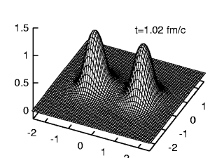
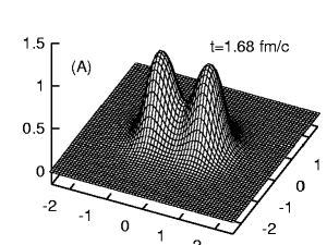
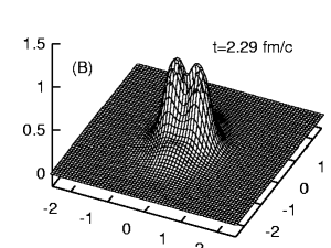
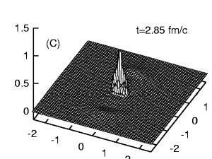
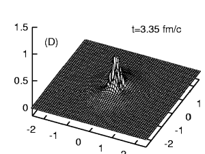
Figure 1: One component of the pion field $(1-\Psi_{0})$ at various moments during annihilation. The fields are shown in the $xy$ plane. The $x$ axis is the direction closer to horizontal. The length on the axes is measured in fermi. The quantity we plot is dimensionless. Note the different vertical and horizontal scales in the last two frames.

The process is best illustrated by the time evolution of the pion field. In Figure 1 we plot the quantity $(1-\Psi_{0})$ as a function of time. This choice is natural since in free space $\Psi_{0}=1$ and at the tip of a Skyrmion $\Psi_{0}=-1$. In the first plot we have the essentially unmodified Skyrmion and anti-Skyrmion, slightly superimposed. The $\Psi_{0}$ component of the pion field is identical for the two objects. Charge conjugation and grooming affects only the ’spatial’ components.

In order to annihilate, the fields have to unwind, therefore the field in the center point has to pass through the value $\Psi=(-1,0,0,0)$ (the highest point in our plots). In other words, the tips must merge before unwinding. The second frame illustrates a moment close to this situation. As will be discussed later, the axial dependence is rather sharp at this moment. In our simulation the symmetry center is between lattice points, therefore the crest in the second frame should be close to horizontal with a proper extrapolation.

From this point on, the value of $\Psi_{0}$ approaches fast the vacuum value as the topological obstacle is now gone. After another fm/c the field is close to the vacuum value $(1,0,0,0)$. The variation is so fast that the field in the center ’overturns’ and increases again. Only after 3 fm/c from the passing of the peak do these large amplitude oscillations subside by propagating outwards as spherical waves. This outgoing pion radiation is clearly seen in the final two frames of Figures 1 and 4.

Figure 2: Evolution of the baryon number in one half-space during a central annihilation process. The points $A\ldots E$ indicate particular moments which are also indicated in Figure 1, 3, and so on, and are referred to throughout the text. Note especially the point $B$, which corresponds to ’half-annihilation’. It is associated with the merging of two topological centers and also marks the beginning of the violent part of the annihilation process.

The time evolution of the baryon number is illustrated in Fig.2. We compute the baryon number by integrating (5) in one half-space. The baryon number in the other half space is equal and opposite to this. The annihilation starts basically when the Skyrmions touch, at $t=1.66\rm\;fm$ (point $A$ in Fig.2). In the absence of interactions, exactly half of the baryon number in one half space should annihilate when the two centers coincide, at $t=3.0\rm\;fm\!/\!c$ . Because of the attractive interaction, this happens a little faster, at around $t=2.3\rm\;fm\!/\!c$ ($B$). Along with the field, the remaining baryon number decreases quickly to zero ($t=2.85\rm\;fm\!/\!c$, point $C$), continues to decrease for a short time, then oscillates, hitting an absolute minimum at point ($D$). The baryon number oscillates along with the large amplitude oscillations of the field and finally settles at zero ($t=5.5\rm\;fm\!/\!c$, point $E$) in the radiation regime.

Altogether, the unwinding of the field (from $A$ to $C$) takes approximately $1.2\ldots 1.3\rm\;fm\!/\!c$, but this is followed by localized oscillations which take a longer amount of time ($C$ to $E$, approximately $2.5\rm\;fm\!/\!c$), therefore the total process from the moment when the Skyrmions touch to the complete disappearence of the baryon number takes about $3.5\rm\;fm\!/\!c$, depending on the choice of the point $E$.

Figure 3: Evolution of the energy and its components during a central annihilation process.

In Fig.3 we plot the evolution of the energy as the sum of the energy in the pion field and the omega field. The dotted lines and labels $A\ldots E$ on Fig.3 indicate the same times as in Fig.2. Our definitions of the energy densities – which are integrated numerically to give the quantities in Figure 3 – are

$${\cal H}_{\pi}~{} = ~{}\frac{1}{2}\left(\dot{\Psi}^{A}\dot{\Psi}^{A}+\sum\limits_{k=1}^{3}\partial_{k}\Psi^{A}\partial_{k}\Psi^{A}\right)$$

$${\cal H}_{\omega}~{} = ~{}\frac{1}{2}\sum\limits_{k=1}^{3}\left(M_{\omega}^{2}\omega_{k}^{2}+{\cal M}_{k}^{2}+{\cal E}_{k}^{2}\right)+\frac{1}{2}M_{\omega}^{2}\omega_{0}^{2}~{}~{}.$$ (18)

The piece corresponding to the $\omega_{0}$ field can be defined in terms of our dynamical variables,

$${\cal H}_{\omega_{0}}~{} = ~{}\frac{1}{2}M_{\omega}^{2}\omega_{0}^{2}=\frac{1}{2M_{\omega}^{2}}\left[\left(\frac{3g}{2}B_{0}\right)-\left(\partial_{k}{\cal E}_{k}\right)\right]^{2}~{}~{}.$$ (19)

The second identity follows from the equations of motion for $\omega_{0}$, the definition of ${\cal E}_{k}$, and the gauge condition. We also plot the total energy in Fig.3. There is a loss of less then $100\rm\;MeV$ from a total of $1500\rm\;MeV$ between the points $B$ and $E$, which corresponds to approximately $7\%$. We assign this loss to numerical dissipation which is significant in the fast-varying regime between half-annihilation ($B$) and the onset of the radiation regime ($E$). The further decay of the total energy simply corresponds to outgoing radiation which leaves the simulation box.

The annihilation process is accompanied by the rearrangement of the energy between the pion and omega sectors. Initially we have free-space propagation of the solitons. The smooth part of the unwinding beginning at ($A$) is accompanied by the flow of energy from the pion field into the omega sector. The net flow stops before full unwinding ($C$) and yields to oscillations which correspond in time to the large oscillations of the field, accompanied by significant oscillations of the baryon number around zero. During this regime, when the net baryon number oscillates, the energy also flows back and forth between the two sectors. Eventually the two sectors stabilize after $E$ at comparable values.

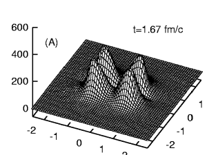
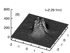
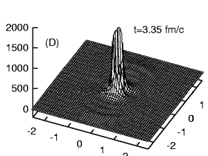
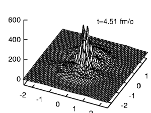
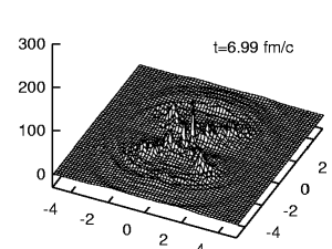
Figure 4: The total energy density multiplied by the distance to the symmetry axis, in $\rm\;MeV/\rm\;fm^{2}$ at various moments during annihilation. The density is shown in the $xy$ plane. The $x$ axis is the direction closer to horizontal. The length on the axes is measured in fermi. Note the different vertical and horizontal scales in the last two frames.

A more detailed picture of the energy flow is given by looking at the spatial distribution of the energy at various moments. In Figure 4 we plot the total energy density multiplied with the distance $\rho$ to the symmetry axis. Plotting $\rho\times dE/dV$ gives a better estimate of the relative amount of energy contained in different regions of space. In the first three frames we see the two configurations approaching each other, then merging. The void in the middle of each lump is due to the fact that we multiplied the energy density with the distance to the $x$ axis. In spite of this, later on the strength is concentrated in the center. Eventually the energy starts to flow outwards in almost spherical waves.

These plots reveal two important aspects. First, the fact that the energy density is very high in the center between $t=3.0\rm\;fm\!/\!c$ and $t=5.0\rm\;fm\!/\!c$, which is the period between annihilation and the start of significant outward energy flow. Note the higher enegy scale on the middle three plots. The other important feature is the abundance of fast, small amplitude oscillations which persist to the end of the time interval under consideration. They can be seen well in the last three plots. These oscillations originate in the period immediately following annihilation when there is a very fast, global variation of the fields confined to a small region of space. Most likely numerical error stemming from the large local variations has a role as a source for these oscillations. However, as discussed in the next subsection on numerical stability, the persistence of the small oscillations is also possibly due to properties of the exact, continuum equations of motion.

Despite the presence of the small oscillations, there is a well defined pattern to the flow of energy, both in terms of radial flow and angular distribution. Starting with $t=2.5\rm\;fm\!/\!c$, the energy is concentrated in a small region (initially of radius $1\rm\;fm$) around the center. The distribution becomes very strongly peaked in the time between half-annihilation and complete unwinding. There is some outgoing radiation as early as $t=3.5\rm\;fm\!/\!c$ but the strongly peaked pattern eases up only after $t=5.0\rm\;fm\!/\!c$ when the bulk of the energy starts flowing outward.

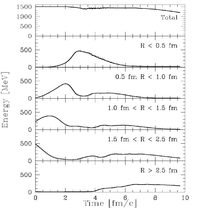
Figure 5: Total energy in spherical shells surrounding the annihilation as a function of time.

The macroscopic flow of energy is nicely illustrated in Fig.5 by plotting the total energy contained in spherical shells surrounding the center. Initially we have the two incoming solitons which move through bins in decreasing order of the radius. Starting from $t=2.5\rm\;fm\!/\!c$ the energy accumulates in the center bin (a sphere of radius $0.5\rm\;fm\!/\!c$, half the linear size of a Skyrmion). The accumulation peaks at about $t=3\rm\;fm\!/\!c$ when this bin contains more than $2/3$ of the total energy. Even though the outward flow starts as early as $t=3.0\rm\;fm\!/\!c$, it becomes significant only later. Approximately $90\%$ of the energy leaves the center sphere by $t=6.0\rm\;fm\!/\!c$ , or $3.0\rm\;fm$ after full unwinding. From then on, we can follow the energy moving outwards through bins of increasing radius. We can also understand how the decrease in total energy (top panel, same line as in Fig.3) is really just flow leaving the simulation box.

Figure 6: Total energy in angular intervals measured from the symmetry axis at various moments during annihilation.

Figure 7: The baryon number density (dotted) and the $x$ component of the baryon current density (solid), integrated over $y$ and $z$ (in $\rm\;fm^{-1}$ respectively ${\rm c}/\rm\;fm$), as a function of the $x$ coordinate, at various moments during the annihilation process.

Finally, in Figure 6 we illustrate the angular distribution of the energy during the annihilation process. In Fig.6 we can see a depletion of the small angle bins, and a peak around $45^{o}$ which seems to be the preferred direction of the energy flow. It should be noted that these angular distributions are in a plane, but that the three dimensional distribution has cylindrical symmetry about the direction of collision.

3.3 Checks

In this subsection we investigate the extent to which our results are influenced by the details of the numerical calculation. This aspect is particularly important because of the presence of large time and spatial derivatives of the fields. The macroscopic dynamics of the problem impose a certain mimimum size for the simulation box (a cube of size $5\rm\;fm$). We use a fixed grid. This limits the number of points per fermi we can have to not much more than 20. Our typical calculations use 12 points per fermi.

One obvious concern stems from the fact that we were able to ensure energy conservation only to about $7\%$, at best $5\%$. Approximately $70\ldots 100\rm\;MeV$ of the total initial energy of $1500\rm\;MeV$ is lost to numerical dissipation, as can be seen in Figs.3 and 5. This loss comes between the points $B$ and $C$ in the respective plots, and is a significant but not alarming energy loss.

Numerical error is probably also responsible for the appearence of persistent but random oscillations. Starting with $t=4.0\rm\;fm\!/\!c$, the field configurations display oscillations on the scale of a few lattice spacings. This is preceded by a configuration which is probably singular in the continuum limit, at half-annihilation (we discuss this in a separate section). This raises the question of whether the continuum physics we wish to study mixes with lattice artifacts, or rather, whether we are at able to extract continuum physics reliably.

To test the stability of our results, we performed several runs using the $\pi$ algorithm for a number of different lattice spacings. The results obtained with this algorithm with identical box size and initial conditions are very similar to those obtained with the $\Psi$ algorithm. The program based on the $\pi$ algorithm has been readily available for a longer time, and we used it for the very time consuming runs with larger numbers of points. Below we present results for 12, 16 and 20 points per fermi. The physical process in these runs is the same, i.e., head-on annihilation with the same parameters as in the main run, initial separation of $3\rm\;fm$, initial velocity of $\beta=0.5$. However, we used the smallest possible simulation box, only $6\times 5\times 5\rm\;fm^{3}$, and a slightly different initial configuration. Using an even smaller box would have resulted in more energy dissipation outside the box, and most notably, reflection off the walls (which we are unable to eliminate completely) which would interfere with the ’real’ physics. We then compared the results from these various runs. Ideally, the numerical artifacts should scale away as the lattice spacing is decreased.

Figure 8: The total energy during the more violent part of the annihilation process, in three calculations which are identical except for the number of points per fermi, $N$. Note that these runs are slightly different from the runs discussed in the preceding section. They are performed in a smaller box using a slightly different initial configuration.

In Figure 8 we plot the total energy for three runs which are identical (including the timestep, which is decreased before $t=3.0\rm\;fm\!/\!c$ from $100$ per fermi to $3200$ per fermi/c) except for the lattice spacing which is respectively $N=12,16,20$ points per fermi. We zoomed in to the region between $t=2.0\rm\;fm\!/\!c$ and $t=5.0\rm\;fm\!/\!c$, when most of the dissipation takes place. The energy decreases as the system is squeezed into the small region around the center. The loss is likely to be caused by discretization error. However, as the system expands, only a fraction of the loss is recovered. The same run with $N=8$ points per fermi, which we cannot plot on the same graph without making the graph completely unintelligible, gives worse conservation than all three runs plotted here. The two larger spacings do give better energy conservation then the $N=12$ run, as one would expect. However, there is no clear scaling, as the order of the $N=16$ and $N=20$ results is reversed. As an argument for the reliability of our calculations, let us emphasize that we are talking about differences of $30\rm\;MeV$ here between calculations, i.e., $2\%$ of the total energy.

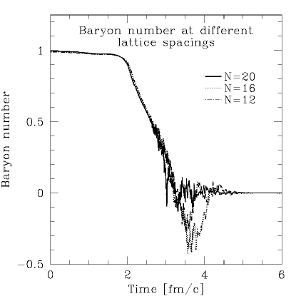
Figure 9: The baryon number in one half space during the annihilation process, in three calculations which are identical except for the number of points per fermi, $N$. Note that these runs are slightly different from the runs discussed in the preceding section. They are performed in a smaller box using a slightly different initial configuration.

A look at the comparative plot of the baryon number in the same runs reveals a similar picture. In all three runs shown, the remarkable points $A$,$B$, $C$ and $E$, i.e., the start of the unwinding, the point of half-annihilation and full unwinding, as well as the end of the violent fluctuations, practically coincide. However, the extent and duration of the excursion of the baryon number below zero varies. It is practically absent for $N=8$ but there is a large fluctuation later on (again, not plotted). For $N=12$ and $N=16$ we see a sizeable excursion, larger for $N=16$, but again the $N=20$ calculation is out of sequence and has only a small negative excursion. It could be that the timestep choice (same for all runs) is too large for $N=20$. Even with this in mind, the overall evolution of the baryon number is very similar for the four runs we discussed. The decay of the baryon number and the duration of the large oscillations is a robust feature of the calculation. Furthermore the small oscillations seem to be very noisy with little relationship from grid size to grid size.

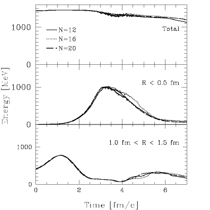
Figure 10: Evolution of the energy contained in a few spherical shells for various lattice spacings.

The outward energy flow is perhaps the most important quantitative result one may extract from a numerical calculation of Skyrmion-anti-Skyrmion annihilation. This result would be the starting point for constructing the final pion and omega states in a calculation of low energy $N\bar{N}$ annihilation [5]. In Figure 10 we plot the energy contained in centered spherical shells, for the three $N=12,16,20$ calculations discussed above. The evolution of the energy contained in the shells is practically the same for the three runs. There is some fluctuation, especially for the center bin, but the differences are not very large. In particular there is little difference in the bins at larger distance, and that is where information would be extracted for the outgoing pion and omega states. We cannot identify a scaling pattern in these cases. However, it is clear that the dominant process of outward flow of energy is well established and is clearly not influenced by variation in the number of lattice points.

In conclusion, our detailed results are somewhat sensitive to the number of lattice points, but the physically important observables, energy conservation, the time evolution of the baryon number, and the flow of energy are reasonably well determined and independent of variations in the number of lattice points.

4 Stability analysis

One of the two most prominent features of our results is the appearence of persistent, small amplitude oscillations after unwinding. These oscillations are present practically to the end of our calculations. In the early post-unwinding regime they influence the total energy and baryon number.

The frequency of the fluctuations of the total energy and baryon number increases with the number of lattice points, suggesting that these are numerical artifacts. We have been forced to use extremely small timesteps in our runs (thousands of timesteps per fermi). However, the precautions we took did not eliminate these oscillations. On the other hand, we are able to perform our simulations to a robust end even in the presence of these oscillations. Furthermore, the macroscopic (long wavelength) aspects of the outputs are not strongly influenced by the number of points, suggesting that numerical artifacts do not overwhelm the continuum physics.

The lack of success of earlier attempts to simulate annihilation [6, 7, 8] has been blamed on a situation which arises in the Skyrme model [6]. Due to the nonlinear nature of the interaction term, the equations of motion may cease to be of hyperbolic nature, i.e., have second time and spatial derivative terms of opposite signs. Hyperbolic equations of motion ensure the existence of plane wave-like solutions (of the form $e^{ik_{\mu}x^{\mu}}$ with real wave numer $k=\sqrt{\vec{k}\cdot\vec{k}}$) which may propagate as packets of quasi constant amplitude. If the sign of the second time derivative reverses, the wave number may become imaginary for a given wave vector $\vec{k}$, resulting in waves with exponentially increasing amplitude. A small fluctuation that excites this mode would then result in a large change in the final result. In other words, if the equations of motion are not hyperbolic, the system in unstable. For a deatiled derivation of the intability for the Skyrme model of just this sort, we refer to [6].

In the following we investigate the possibility of such an instabiliy occuring in our model. Recall that we are using $\omega$ stabilization rather than a Skyrme term in order to avoid the damage brought on by the fourth-order interaction term. Consider our equations of motion,

$$\partial_{\mu}\partial^{\mu}\Psi^{A}~{}-~{}\Psi^{A}\left(\Psi^{E}\partial_{\mu}\partial^{\mu}\Psi^{E}\right)~{} = ~{}\frac{3g}{8f_{\pi}^{2}\pi^{2}}\epsilon^{\mu\nu\alpha\beta}\epsilon^{ABCD}\partial_{\nu}\omega_{\mu}\Psi^{B}\partial_{\alpha}\Psi^{C}\partial_{\beta}\Psi^{D}+m_{\pi}^{2}\left(\delta^{A0}-\Psi^{0}\Psi^{A}\right)$$

$$\partial^{\nu}\partial_{\nu}\omega^{\mu}~{} = ~{}\frac{g}{8\pi^{2}}\epsilon^{\mu\nu\alpha\beta}\epsilon^{ABCD}\partial_{\nu}\Psi^{A}\Psi^{B}\partial_{\alpha}\Psi^{C}\partial_{\beta}\Psi^{D}-M^{2}\omega^{\mu}$$ (20)

Consider now a solution of these equations and a small, fast-varying perturbation added to it,

$$\Psi^{A}~{} \rightarrow ~{}\Psi_{0}^{A}~{}+~{}\epsilon\phi^{A}~{}~{};~{}~{}|\partial_{\mu}\phi^{A}|>>|\partial_{\mu}\Psi^{A}|$$

$$\omega^{\mu}~{} \rightarrow ~{}\omega_{0}~{}+~{}\epsilon\sigma^{\mu}~{}~{};~{}~{}|\partial_{\mu}\sigma_{\nu}|>>|\partial_{\mu}\omega_{\nu}|$$ (21)

where $\epsilon$ is a small real number. We study the stability of the equations of motion by analyzing the behavior of these small perturbations in the background field given by $\left\{\Psi^{A},\omega^{\nu}\right\}$. First, we substitute the ansatz (4) into the equations of motion and expand to first order in $\epsilon$,

$$\partial_{\mu}\partial^{\mu}\phi^{A}~{} + ~{}\phi^{A}\left(\partial_{\mu}\Psi^{E}\partial^{\mu}\Psi^{E}\right)~{}+~{}2\Psi^{A}\left(\partial_{\mu}\phi^{E}\partial^{\mu}\Psi^{E}\right)~{}=~{}$$

$$= ~{}\frac{3g}{8\pi^{2}f_{\pi}^{2}}\epsilon^{\mu\nu\alpha\beta}\epsilon^{ABCD}\left\{\partial_{\nu}\sigma_{\mu}\Psi^{B}\partial_{\alpha}\Psi^{C}\partial_{\beta}\Psi^{D}~{}+~{}\partial_{\nu}\omega_{\mu}\left(\phi^{B}\partial_{\alpha}\Psi^{C}\partial_{\beta}\Psi^{D}~{}+~{}2\Psi^{B}\partial_{\alpha}\phi^{C}\partial_{\beta}\Psi^{D}\right)\right\}$$

$$~{}~{}~{}~{}-2m_{\pi}^{2}\left(\phi^{A}\Psi^{0}+\Psi^{A}\phi^{0}\right)~{}~{}$$

$$\partial_{\nu}\partial^{\nu}\sigma^{\mu}~{} = ~{}\frac{3g}{8\pi^{2}}\epsilon^{\mu\nu\alpha\beta}\epsilon^{ABCD}\left(\partial_{\nu}\phi^{A}\Psi^{B}+\frac{1}{3}\partial^{\nu}\Psi^{A}\phi^{B}\right)\partial_{\alpha}\Psi^{C}\partial_{\beta}\Psi^{D}~{}~{}~{}.$$ (22)

We must again remember that the variation of $\Psi$ is constrained,

$$(\Psi^{A}+\epsilon\phi^{A})(\Psi_{A}+\epsilon\phi_{A})~{}=~{}1~{}+~{}{\cal O}(\epsilon^{2})~{}~{}\rightarrow~{}~{}\phi^{A}\Psi^{A}~{}=~{}0~{}~{}.$$ (23)

Therefore the quantity $\epsilon^{ABCD}\partial_{\nu}\Psi^{A}\phi^{B}\partial_{\alpha}\Psi^{C}\partial_{\beta}\Psi^{D}$ has to vanish since it is the quadruple product of four isospin vectors which are all perpendicular ot ${\bf\Psi}$.

We now assume that small perturbations are well approximated by plane waves,

$$\phi^{A}~{}=~{}\Phi^{A}e^{ik_{\mu}x^{\mu}}~{}~{};~{}~{}\sigma^{\nu}~{}=~{}\Sigma^{\nu}e^{ik_{\mu}x^{\mu}}~{}~{},$$ (24)

and attempt to obtain equations for the wave vector $k_{\mu}$. If the equations have solutions which correspond to an imaginary $k_{0}=\Omega$, then we conclude that our equations of motion are unstable, since they allow for the exponential increase of a small perturbation. After substituting the ansatz (24) into (4) and contracting the first equation with $\Phi^{A}$ we obtain

$$-k_{\mu}k^{\mu}+M_{\perp}^{2}+2m_{\pi}^{2}\Psi^{0}~{} = ~{}\frac{3g}{8\pi^{2}f_{\pi}^{2}}ik_{\nu}\Sigma_{\mu}\epsilon^{\mu\nu\alpha\beta}\epsilon^{ABCD}\Phi^{A}\Psi^{B}\partial_{\alpha}\Psi^{C}\partial_{\beta}\Psi^{D}$$

$$\left(-k_{\nu}k^{\nu}+M^{2}\right)\Sigma^{\mu}~{} = ~{}\frac{3g}{8\pi^{2}}ik_{\nu}\epsilon^{\mu\nu\alpha\beta}\epsilon^{ABCD}\Phi^{A}\Psi^{B}\partial_{\alpha}\Psi^{C}\partial_{\beta}\Psi^{D}~{}~{}.$$ (25)

Here we took advantage repeatedly of the perpendicularity of ${\bf\Phi}$ to ${\bf\Psi}$. We also defined $M_{\perp}^{2}=\partial_{\mu}\Psi^{E}\partial^{\mu}\Psi^{E}$ . Note that this quantity originates in the constraint on ${\bf\Psi}$ and is not necessarily positive definite. This in itself does not imply the appearence of an instability, since in the static case, which is free of instabilites against small oscillations, $M_{\perp}<0$. We should of course take the sign of $M_{\perp}$ into account when we analyze the characteristic equation.

Let us solve the second equation for the polarization vector $\Sigma^{\mu}$ and substitute into the first equation. The result can be rearranged as follows

$$\left(-k_{\mu}k^{\mu}+M^{2}\right)\left(-k_{\rho}k^{\rho}+M_{\perp}^{2}+2m_{\pi}^{2}\Psi^{0}\right)~{} = ~{}-\left(\frac{3g}{8\pi^{2}f_{\pi}}\right)^{2}k_{\nu}k_{\rho}~{}\epsilon^{\mu\nu\alpha\beta}\epsilon_{\nu~{}~{}~{}}^{~{}\rho\sigma\tau}V_{\alpha\beta}V^{\sigma\tau}$$

$$= ~{}-\left(\frac{3g}{8\pi^{2}f_{\pi}}\right)^{2}k_{\nu}k_{\rho}~{}S^{\mu\nu}S_{\mu~{}}^{~{}\rho}$$ (26)

where we have defined $V_{\alpha\beta}~{}=~{}\epsilon^{ABCD}\Phi^{A}\Psi^{B}\partial_{\alpha}\Psi^{C}\partial_{\beta}\Psi^{D}$ and $S^{\mu\nu}~{}=~{}\epsilon^{\mu\nu\alpha\beta}V_{\alpha\beta}$ .

As for any Lorentz tensor of rank 2, there are two invariants one may construct from the components of $S^{\mu\nu}$, $A~{}=~{}\epsilon^{\mu\nu\alpha\beta}S_{\mu\nu}S_{\alpha\beta}$ and $B~{}=~{}S^{\mu\nu}S_{\mu\nu}$ . If $A=0$, then using the appropriate Lorentz boost, the tensor can be either brought to a form where the ’electric’ components $S^{0k}$ vanish or it can be brought to a form where the ’magnetic’ components $S^{lm}$ vanish. Only one of these situations is possible, depending on the sign of the other invariant. If $B<0$ the tensor is ’electric’, and if $B>0$ it is ’magnetic’. Let us compute the first invariant,

$$A~{} = ~{}\epsilon^{\mu\nu\alpha\beta}\epsilon_{\alpha\beta\rho\sigma}\epsilon_{\mu\nu\lambda\tau}V^{\rho\sigma}V^{\lambda\tau}~{}=~{}2\epsilon_{\mu\nu\lambda\tau}V^{\mu\nu}V^{\lambda\tau}$$ (27)

$$= ~{}2\epsilon^{ABCD}\epsilon^{EFGH}\Phi^{A}\Psi^{B}\Phi^{E}\Psi^{F}\epsilon^{\mu\nu\alpha\beta}\partial_{\mu}\Psi^{C}\partial_{\nu}\Psi^{D}\partial_{\alpha}\Psi^{G}\partial_{\beta}\Psi^{H}~{}~{}.$$

Consider one set of values for the eight isospin indices on the right hand side. For a nonvanishing term, the labels $\left\{C,D,G,H\right\}$ must be all different, otherwise we would have symmetry in two Greek indices. For simplictiy let $\left\{C,D,G,H\right\}=\left\{0,1,2,3\right\}$ . The Lorentz sum remaining to be performed can be rearranged,

$$\epsilon_{0123}\epsilon^{\mu\nu\alpha\beta}\partial_{\mu}\Psi^{0}\partial_{\nu}\Psi^{1}\partial_{\alpha}\Psi^{2}\partial_{\beta}\Psi^{3}~{}=~{}\epsilon_{ABCD}\epsilon^{0123}\partial_{0}\Psi^{A}\partial_{1}\Psi^{B}\partial_{2}\Psi^{C}\partial_{3}\Psi^{D}~{}=~{}0~{}~{}.$$ (28)

The term on the right hand side vanishes because it contains four isovectors perpendicular to $\Psi$. Hence the first invariant vanishes. The second invariant is

$$B~{} = ~{}S^{\mu\nu}~{}S_{\mu\nu}~{}=~{}\epsilon^{\mu\nu\alpha\beta}\epsilon_{\mu\nu\rho\sigma}V_{\alpha\beta}V^{\rho\sigma}~{}=~{}$$ (29)

$$= ~{}-2V_{\alpha\beta}V^{\alpha\beta}~{}=~{}2\left[V_{0k}V_{0k}-V_{lm}V_{lm}\right]~{}~{}$$

$$= 2\epsilon^{ABCD}\epsilon^{EFGH}\Phi^{A}\Psi^{B}\Phi^{E}\Psi^{F}\left[2\dot{\Phi}^{C}\partial_{k}\Psi^{D}\dot{\Phi}^{G}\partial_{k}\Psi^{H}-\partial_{l}\Psi^{C}\partial_{k}\Psi^{D}\partial_{l}\Psi^{C}\partial_{k}\Psi^{D}\right]~{}~{}.$$

In the last line we have lowered all Lorentz indices. ( We remind the reader of our convention $A_{\mu}=(A_{0},\vec{A});A^{\mu}=(A_{0},-\vec{A})$ . ) It is clear that if the time-derivatives are small, $B<0$ and if they are large, i.e., for fast-varying $\Psi$ fields, $B>0$.

Let us consider the case with small time-derivatives. Then, $B<0$ and the tensor $S$ may be boosted so that $S_{lm}=0$ . The characteristic equation is then

$$(M^{2}-k_{\mu}k^{\mu})(M_{\perp}^{2}+2m_{\pi}^{2}\Psi^{0}-k_{\nu}k^{\nu})~{}=~{}-2{\cal C}^{2}\left\{k_{0}k_{0}S^{l0}S^{~{}0}_{l~{}}+k_{l}k_{m}S^{0l}S^{0m}\right\}$$

$$(M^{2}+p^{2}-\omega^{2})(M_{\perp}^{2}+2m_{\pi}^{2}\Psi^{0}+p^{2}-\omega^{2})~{}=~{}2{\cal C}^{2}\left\{\omega^{2}\sum\limits_{l}\left(S_{0l}^{2}\right)-p_{l}p_{m}\left(S_{0l}S_{0m}\right)\right\}~{}~{}.$$ (30)

Only the component of $\vec{p}$ parallel to the electric field vector $\left\{E_{k}=S_{0k}\right\}$ contributes to the right-hand side. Denoting that component by $p_{1}$, we have finally

$$(M^{2}+p^{2}-\omega^{2})(M_{\perp}^{2}+2m_{\pi}^{2}\Psi^{0}+p^{2}-\omega^{2})~{}=~{}2{\cal C}^{2}\left(S_{0k}S_{0k}\right)\left(\omega^{2}-p_{1}^{2}\right)~{}~{}.$$ (31)

When the time-derivatives dominate, we have $B>0$ and we may choose a reference frame where $S_{0k}=0$. The corresponding characteristic equation is

$$(M^{2}-k_{\mu}k^{\mu})(M_{\perp}^{2}+2m_{\pi}^{2}\Psi^{0}-k_{\nu}k^{\nu})~{} = ~{}-2{\cal C}^{2}k_{l}k_{m}S^{jl}S_{j~{}}^{~{}m}$$ (32)

$$= ~{}2{\cal C}^{2}p_{l}p_{m}S_{jl}S_{jm}~{}=~{}2{\cal C}^{2}\sum\limits_{j}\left(\sum\limits_{l}p_{l}S_{jl}\right)^{2}\geq 0~{}~{}.$$

The matrix ${\cal W}_{lm}=S_{jl}S_{jm}$ can be diagonalized $\tilde{\cal W}_{lm}=\delta_{lm}w_{l}$ and its eigenvalues will be real and positive as it is obvious from the preceding equation. In that basis, the characteristic equation is

$$(M^{2}+p^{2}-\omega^{2})(M_{\perp}^{2}+2m_{\pi}^{2}\Psi^{0}+p^{2}-\omega^{2})~{}=~{}2{\cal C}^{2}\sum\limits_{l}p_{l}^{2}w_{l}~{}~{}.$$ (33)

The characteristic equations in the $B<0$ and $B>0$ cases can be summarized as follows:

$$(M_{1}^{2}+p^{2}-\omega^{2})(M_{2}^{2}+p^{2}-\omega^{2})~{} = ~{}K_{1}^{2}(\omega^{2}-P_{1}^{2})~{}~{}~{};~{}~{}[B<0]$$

$$(M_{1}^{2}+p^{2}-\omega^{2})(M_{2}^{2}+p^{2}-\omega^{2})~{} = ~{}K_{2}^{2}P_{1}^{2}~{}~{}~{};~{}~{}[B>0]~{}~{}~{}.$$ (34)

Here, $p^{2}$ and $P_{1}^{2}$ are respectively the square and the square of one component of the arbitrary wave vector $\vec{p}=\vec{k}$ associated with the plane-wave perturbation. The quantities $K_{1}^{2}$ and $K_{2}^{2}$ are positive real numbers, and so is $M_{1}^{2}=M_{\omega}^{2}$. The only exception is $M_{2}^{2}=M_{\perp}^{2}+2m_{\pi}^{2}\Psi^{0}\approx M_{\perp}^{2}=\partial_{\mu}\Psi^{E}\partial^{\mu}\Psi^{E}$. As we have mentioned, $M_{\perp}^{2}$ is negative for a static field configuration such as a Skyrmion at rest, which does not exhibit a proliferation of small-wavelength perturbations. $M_{\perp}^{2}$ becomes positive when the time derivatives become large. This is the case in the center between the moments ($B$) and ($E$) (as defined in Sec.3), when most of the violent behavior takes place. It is clear from the sign of $M_{\perp}^{2}$, as well as from the following discussion, that the characteristic equations allow for a complex $\omega$ in a number of dynamical situations. We will focus on the regime between the moments ($B$) and ($E$) and assume $M_{\perp}^{2}>0$, and look for the conditions that are consistent with a negative $\omega^{2}$.

In both cases ($B>0$ or $B<0$) we have a quadratic equation for $\omega^{2}$. We may solve the characteristic equation for the time constant $\omega=k_{0}$ using any given $\vec{p}$. We remind the reader the we are studying the possiblity of having a complex time constant. Such a perturbation would grow or decrease exponentially with time. When the right-hand side is small, both solutions, $\omega^{2}=M_{1}^{2},M_{2}^{2}$ are real and positive, leading to stable oscillations.

In the $B<0$ case, the r.h.s. has the effect of increasing both the coefficient of $\omega^{2}$ (in absolute value) and the free term. Considering the solutions of a quadratic equation $aX^{2}-bX+c=0$ (all coefficients are positive here), $X_{12}~{}=~{}\left((-b\pm\sqrt{b^{2}-4ac}\right)/2a$ it is clear that increasing $b$ (if both $a$ and $c$ are positive) can make the positive real roots neither negative nor complex. Increasing $c$ actually has the effect of bringing the roots closer together, therefore increasing the lower one. This may lead to trouble if the coefficient $c\geq b^{2}/4a$, however, this is not possible as it is obvious if one writes the discriminant out explicitely. We conclude that in this case, both solutions for $\omega^{2}$ are real and positive, leading only to stable modes.

In the $B>0$ case there is no term containing $\omega$ on the right-hand side. However, the free term has the opposite sign compared to the previous case. It may not make the discriminant negative since it decreases $c$. However, if large enough in magnitude, this term may change the sign of $c$, thus allowing for a negative solution for $\omega^{2}$ .

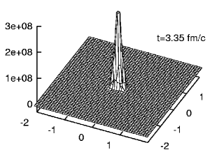
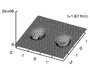
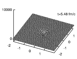
Figure 11: The highest (top row) and the lowest (bottom row) eigenvalue of the tensor ${\cal T}$ at selected moments during annihilation. The unit for the eigenvalues is ${\rm c^{2}}/\;\rm\;fm^{4}$. Note the large differences in the vertical scales. We plot the quantities in the $xy$ plane. The $x$ axis is the direction closer to horizontal. The length on the axes is measured in fermi.

We conclude that if $M_{\perp}^{2}>0$, modes with purely imaginary $\omega^{2}$ may occur in the $B>0$ case. This makes sense, because this case is associated with large time derivatives, exactly what characterizes our violent regime. The latter is also consistent with the assumption $M_{\perp}^{2}>0$. The sign of $B$ is not immediately obvious, since it also depends on the polarization vector of the supposed perturbation, $\Phi^{A}$: $B=\Phi^{A}\Phi^{B}{\cal T}^{AB}$, where all the background-field dependent factors are contained in the tensor ${\cal T}$. If all eigenvalues of ${\cal T}$ are negative, $B<0$ for any polarization. If there is one positive eigenvalue, then it is possible to have $B>0$. If all eigenvalues are positive, $B>0$ for any polarization vector. In Figure 11 we plot the highest and the lowest eigenvalues of ${\cal T}$ before, during and after the violent oscillation regime. This illustrates that during free propagation the negative eigenvalues dominate, while during the violent regime, the eigenvalues, and also $B$ become very large in absolute value, and the positive eigenvalues dominate. Towards the end of the process, the $B>0$ regime lingers close to the center but is not present in the outgoing radiation. In Figure 12 we plot the absolute values of the largest and lowest eigenvalues of ${\cal T}$ in the whole simulation box as a function of time. The moment of half-annihilation ($B$) marks a significant increase in the magnitude of the positive eigenvalues, which dominate in the center region through the remainder of the calculation.

Figure 12: The absolute values of the lowest (usually negative) and highest (usually positive) eigenvalue of the tensor ${\cal T}$ overall during annihilation, in ${\rm c}^{2}/\;\rm\;fm^{4}$. We associate the presence of large positive eigenvalues of ${\cal T}$ with instability against perturbations.

In summary, the equations of motion allow in principle for the appearence of exponentially growing perturbations. The conditions for this are rather specific. We are able to show that such conditions accompany the violent, fast-varying regime that follows the unwinding and persist until the outgoing radiation phase. However, we cannot establish a clear, causal connection between the $B>0$ regime and the fluctuations.

5 Singular behavior

The source of the persistent small oscillations is the fast-varying behavior that follows the point of half-annihilation. The fields at this point and shortly afterwards are singular, or close to that. This is the single most prominent feature of the head-on annihilation process. The few off-center calculations we performed show very similar features.

The head-on annihilation process has axial symmetry. In this case, the four ’Cartesian’ components of the pion field are of the form

$$\Psi_{0}(x,y,z,t)~{}=~{}f(x,\rho,t)~{} : ~{}\Psi_{1}(x,y,z,t)~{}=~{}g(x,\rho,t)$$

$$\Psi_{2}(x,y,z,t)~{}=~{}\frac{y}{\rho}h(x,\rho,t)~{} : ~{}\Psi_{3}(x,y,z,t)~{}=~{}\frac{z}{\rho}h(x,\rho,t)$$ (35)

where $\rho=\sqrt{y^{2}+z^{2}}$ and the chiral constraint is $f^{2}+g^{2}+h^{2}=1$. The components of $\omega_{\mu}$ have a similar dependence. The three components of $\Psi$ have additional symmetry constraints, namely they are all even functions of $x$. The radial dependence at $\rho\rightarrow 0$ inherits the symmetry properties of $\Psi$, $\Psi_{0}$ and $\Psi_{1}$ being even functions of $y$ and $z$ while $\Psi_{2}(-y)=-\Psi_{2}(y)$ and $\Psi_{3}(-z)=-\Psi_{3}(z)$ . Therefore $f$ and $g$ are ’even’ and $h$ is and ’odd’ function of $\rho$, in the sense that $h_{|\rho=0}=0$ and $\partial_{\rho}f_{|\rho=0}=\partial_{\rho}g_{|\rho=0}=0$ when the respective functions are continuous.

Let us consider the $\rho=0$ axis, where only $f$ and $g$ can be non-zero. At $x=\pm\infty$ , in free space, we have $f=1$ . As one passes through a Skyrmion, the two components ’rotate’, so that in the center of the Skyrmion we have $f=1$. Similarly, if we choose to move through the $\rho$ direction through the center of the same Skyrmion, the $g$ component would have to vanish by symmetry and the rotation would happen in the $fh$ plane.

The moment of half-annihilation corresponds to the situation when the centers of the Skyrmion and the anti-Skyrmion coincide, i.e., $f=-1$ at $x=0$ . Now let us consider the radial dependence in the $x=0$ plane at this moment. At $\rho=0$ we have $f=-1$, $g=0$, and $h=0$. At $\rho=\infty$ we have again $f=1$, $g=0$, $h=0$ . In this case however, the rotation happens involving mostly the $f$ and the $h$ components. At least close to $\rho=0$, $g$ must be much smaller than $h$, since its first $\rho$ derivative must vanish.

Figure 13: Pion field $(1-\Psi_{0})$ close to half-annihilation. Extrapolating the field to the center would result in a discontinuity in the derivative. The fields are shown in the $xy$ plane. The $x$ axis is the direction closer to horizontal. The length on the axes is measured in fermi. The quantity we plot is dimensionless.

In Figure 13 we plot $(1-\Psi^{0}(x,y))/2=(1-f)/2$, at a moment close to half-annihilation. The field at the center point is close to $f=-1$. As we move outwards along the $y$ (radial) axis, $1-f$ decreases. Notice that the variation of $f$ is is concentrated for the most part in a small region around $\rho=0$. In apparent contradiction with the requirement that $f(y)$ should be an even function, (hence, $\partial_{y}f=0$ at $y=0$), $\partial_{\rho}f=\partial_{y}f$ increases in magnitude as $y\rightarrow 0$. The $\rho$-dependence of $f$ in Figure 13 is well approximated by a $\rho^{\alpha}$ with $\alpha=0.2\ldots 0.3$. The energy density and the baryon current are both determined by the first derivatives of $\Psi^{A}$. The effect is more dramatic in terms of these quantities.

Figure 14: The baryon number density (in $\rm\;fm^{-3}$), the $x$ component of the baryon current density (in ${\rm c}/\rm\;fm^{3}$), and the energy density ( in $\rm\;MeV/\rm\;fm^{3}$) close to the point of half-annihilation. The fields are shown in the $xy$ plane. The $x$ axis is the direction closer to horizontal. The length on the axes is measured in fermi.

In Figure 14 we plot the baryon number density, the $x$ component of the baryon current density, and the energy density in the $xy$ plane. The baryon current is concentrated in a very narrow region in the $x=0$ plane, and the energy density has a steep peak that will grow dramatically during the fast-varying regime. We wish to point out that this situation occurs at half-annihilation, just before the messy part of the annihilation process. It seems very plausible that this quasi-singular configuration is the ultimate source of the turbulence that follows. Because of the presence of this feature we have been forced to place our grid points so that the symmetry center falls halfway between them in all directions, in order to avoid having to deal with inifinite derivatives. We most likely miss the exact moment of the overturn ($f=1$ at $x=\rho=0$). Hence we cannot tell whether the $\alpha\rightarrow 0$ limit is achieved (this implies that $f(\rho)$ is a Heaviside function, and the baryon current is a delta function, i.e., is all concentrated in the center). What is clear is that as the overturn is approached the baryon current concentrates more and more in the center, and that close to that moment, the dependence of the field components is consistent with a small power behavior, which in itself leads to infinite derivatives, hence locally infinite energy density.

A precise understanding of the singular phenomenon described above requires a more focused investigation. At this stage we have a qualitative explanation. Recall that our $\omega$ field, apart from its mass, is an abelian gauge field similar to the electromagnetic field. It couples to the respective components of the baryon current ${\cal B}$ which, in axial geometry, has only three independent components, the baryon density, the $x$ component, and a radial component. The $\omega$ field mediated all interaction in our model. Solitons in the pure nonlinear sigma model collapse because their energy scales as the first power of their linear size. The omega field couples to the baryon (winding number) density. The fact that this stabilizes the Skyrmions against collapse may be interpreted as a consequence of electrostatic repulsion of the baryon charge mediated by the (omega) electric field.

The annihilation process consists of the flow of charges of opposite signs towards the center plane ($x=0$ in our notation), i.e., the presence of a large $B^{1}$ component. The fact that the fields vary fast in the center plane means that the baryon current is concentrated in the center or vice versa. The baryon current is very large in the center and is pushed into a small cross-section in analogy with the electromagnetic ’pinch’ effect enountered in plasmas. This is a consequence of the attractive interaction between parallel electric currents. This effect competes with the electrostatic repulsion of the charge density. The static charge density must vanish in the center plane, by symmetry, (actually, all derivatives of the pion fields with respect to $x$ are zero by symmetry) therefore here the pinch effect is strongest. At the time of half-annihilation there is a further depletion of static charge from the $x=0$ region, which would explain why the pinch effect occurs first at or close half-annihilation.

     

Figure 15: One component of the pion field $(1-\Psi^{0})$ close to half-annihilation, during the true annihilation process and during a calculation where the kinetic energy is periodically depleted by setting time derivatives to zero. The second plot shows no pinching in the middle, indicating that the presence of a baryon current is necessary in order to have a pinch. The fields are shown in the $xy$ plane. The $x$ axis is the direction closer to horizontal. The length on the axes is measured in fermi. The quantity we plot is dimensionless.

To test whether we indeed are looking at an enectromagnetic effect, we performed a ’sticky slope’ calculation, in which we periodically set the time derivatives of the pion field, as well as the magnetic fields, to zero. This also cancels the baryon current, but not the baryon charge, and the annihilation proceeds ’quasistatically’. We followed this process to the points where the baryon number in one half space was $0.55$. In Figure 15 we plot $1-\Psi^{0}$ at this moment in the sticky slope calculation, and, for comparison, the configuration with the same baryon number in a calculation with the same parameters which proceeds normally. The pinching all but disappears in the ’quasistatic’ calculation. This observation is consistent with the contention that the baryon current is responsible for the pinching, since in the sticky slope case there is no current, and as a result the pinching is absent as well.

While the electromagnetic effects offer a qualitative explanation, one would like to have an approach that leads to quantitative understanding, perhaps allowing for an analytical description of the singular part. Furthermore, one may ask the question whether this effect is specific to the omega-stabilized model, or is a general feature of dynamically stabilized solitons.

6 Conclusion and outlook

We have studied the classical process of annihillation of a Skyrmion and an anti-Skyrmion, in a nonlinear sigma model Lagrangian which couples the $SU(2)$ winding number to a vector field ($\omega$). This coupling stabilizes the Skyrmion without some of the short wave length problems inherent in the usual fourth order Skyrme term. Our ultimate goal is to relate classical annihilation to the physical process of nucleon-antinucleon annihillation. In this paper our goal in more modest. It is to show, for the first time, that annihilation in the classical model can be followed numerically from the intial state of separated Skyrmion and anti-Skyrmion to the final state of outgoing pion and omega radiation. We do encounter some violent behavior in our calculation, but it seems to be tamer than the fatal fluctuations previously encountered in Skyrmion annihilation calculations [6, 7]. We are able to follow the calculations from beginning to end with results that are robust and independent of the details of the turbulent behavior.

In this first attempt we only calculate Skyrmion anti-Skyrmion annihilation for head on collisions and only in the most attractive grooming. Our numerical code permits other initial configurations and we plan to come back to them. We find that annihilation happens very rapidly and is accompanied by a sharp (singular) concentration of energy density and baryon current. This causes short wave length, noisy oscillations but we are able to integrate through them. We find a burst of pion and omega radiation peaked in a cone at 45 degrees with respect to the incident direction. We find turbulent behavior but the calculated outgoing meson field radiation carries the total incident energy to within $8\%$. We show analytically that our equations of motion allow for a regime which is unstable with respect to the appearence of exponentially increasing (in time) perturbations. However, these conditions are met only in a spatially and temporally limited part of the system under study. This is one possible reason that the instability does not compromise the simulation. We find that the singular concentration of baryon current associated with annihilation is analogous to the pinch effect in electromagentism. Our theory with a vector field coupled to the current is like electromagentism, but with a mass. We are studying ways to exploit, analytically, the nature of the singularity to control its contribution. It would be interesting to study whether similar singular behavior involving a peaked baryon current occurs in theories like the standard Skyrme model, where there is no relation to electromagnetism.

In the future we plan to study Skyrmion anti-Skyrmion collsions that are not head on and to calculate for other groomings and incident energies. From this we will develop results that can be used to extract predictions for nucleon-antinucleon physics. We also plan to study the singularities we encountered to see if their analytic form can be exploited. It is sometimes the case that in the vicinity of singular behavior one can make precise, analytic statements about solutions to problems that can otherwise only be addressed numerically. It will be interesting to see if that is the case here and to examine how general that approach is. Thus our results suggest ample opportunities for futher work both in nucleon annihilation physics and in mathematical physics.

This work was supported in part by a grant from the United States National Science Foundation. The calculations have been performed mostly on the National Scalable Cluster Center at the University of Pennsylvania. We are grateful to R. Hollebeek for his continued support. We also thank the Eniac 2000 group for allowing us to use their resources for part of this work.

We thank Randy Kamien, Pavlos Protopapas, Krishna Rajagopal, Folkert Tangerman, and Jac Verbaarschot for many useful discussions.

References

- [1] T.H.R. Skyrme, Proc. R. Soc. London 262 (1961) 237; Nucl. Phys. 31 (1962) 556.
- [2] E. Witten, Nucl. Phys. 160, (1979) 57.
- [3] for reviews on the subject of Skyrmions, see I. Zahed, G.E. Brown, Phys. Rept. 142 (1986) 1; T. Gisinger, M.B. Paranjape, Phys. Rept. 306 (1998) 109.
- [4] Y. Lu, P. Protopapas, R.D. Amado, Phys. Rev. C 57 (1998) 1983; Y. Lu, R.D. Amado, Phys. Rev. C 54 (1996) 1566.
- [5] Y. Lu, R.D. Amado, Phys. Rev. C 52 (1995) 2158; B. Shao, R.D. Amado, Phys. Rev. C 50 (1994) 1787.
- [6] W.Y. Crutchfield, J.B. Bell, J. Comp. Phys. 110 (1994) 234.
- [7] H.M. Sommerman, R. Seki, S. Larson, S.E. Koonin, Phys. Rev. D 45 (1992) 4303.
- [8] J.J.M. Verbaarschot, T.S. Walhout, J. Wambach, H.W. Wyld, Nucl. Phys. A461 (1987) 603; J.J.M. Verbaarschot, Phys. Lett. B 195 (1987) 235.
- [9] R. D. Amado, M. Á. Halász, P. Protopapas, Phys. Rev. D 61 (2000) 074022.
- [10] U. G. Meissner, I. Zahed, Phys. Rev. Lett. 56, (1986) 1035.
- [11] D. A. Dwyer and K. Rajagopal, hep-ph/0004126.