Quantum dissipative effects and neutrinos : current constraints and future perspectives

Abstract

We establish the most stringent experimental constraints coming from recent terrestrial neutrino experiments on quantum mechanical decoherence effects in neutrino systems. Taking a completely phenomenological approach, we probe vacuum oscillations plus quantum decoherence between two neutrino species in the channels $\nu_{\mu}\rightarrow\nu_{\tau}$, $\nu_{\mu}\rightarrow\nu_{e}$ and $\nu_{e}\rightarrow\nu_{\tau}$, admitting that the quantum decoherence parameter $\gamma$ is related to the neutrino energy $E_{\nu}$ as : $\gamma=\gamma_{0}\,E_{\nu}^{n}$, with $n=-1,0,1$ and $2$. Our bounds are valid for a neutrino mass squared difference compatible with the atmospheric, the solar and, in many cases, the LSND scale. We also qualitatively discuss the perspectives of the future long baseline neutrino experiments to further probe quantum dissipation.

I Introduction

The striking results of solar [1] and atmospheric [2] neutrino experiments testify, beyond any reasonable doubt, that neutrino physics involves quantum interference phenomena. This is why it is plausible to envisage today the use of neutrino oscillations to probe the foundations of quantum mechanics and, in particularly, to test the completeness of the theory.

From the theoretical point of view, quantum dissipative effects can be viewed either as a consequence of a fundamental violation of quantum physics [3, 4], motivated by quantum gravity, or of an effective description of a micro system weakly coupled to the macroscopic world in a open quantum system framework [5].

In the former approach, it is argued that quantum fluctuations of the gravitational field can lead to a loss of quantum coherence, making time-evolution transform pure quantum states into mixed ones, thereby violating ordinary quantum mechanics [6, 7, 8]. In the latter approach, quantum mechanics is not violated at the level of the global system but rather only by the reduced effective dynamics of the micro subsystem weakly coupled to the macro reservoir [5, 9].

Since both of these attitudes, although conceptually very different, will result in a modification of the time evolution of the neutrino mass eigenstates leading to the appearance of damping factors in the neutrino oscillation probabilities, we will not advocate in favor of either physical interpretation but rather simply treat here the effect phenomenologically. We consider that the absence of a full dynamical theory that can account for the origin, define the energy dependence and ultimately estimate the size of the decoherence effect is a good motivation for phenomenological analyses which can derive, directly from experimental data, limits which are valid independently of the (unknown) theoretical picture.

Bounds on dissipative parameters have already been derived from studies of neutral meson systems [5, 10, 11, 12, 13] and neutron interferometry [14]. A first attempt to use neutrino systems to investigate quantum dissipative effects was reported in Ref. [15]. In Ref. [16], the possibilities of future neutrino experiments to unravel quantum decoherence was qualitatively discussed. Recently, tight limits were obtained in the channel $\nu_{\mu}\rightarrow\nu_{\tau}$ from the atmospheric neutrino data, for a decoherence parameter $\gamma$ which is either supposed to be a constant or proportional to the neutrino energy squared, and in fact a solution to the atmospheric neutrino problem (ANP) was found, when $\gamma$ was suppose to be inversely proportional to the neutrino energy [17]. The quantum decoherence parameter at the best-fit value of this novel solution to the ANP is such that it is not in conflict with other experimental constraints, but it is big enough to explain all the atmospheric neutrino data (sub-GeV, multi-GeV and upward going muons) comparably well as the mass induced $\nu_{\mu}\rightarrow\nu_{\tau}$ oscillation mechanism in vacuum.

In this paper, we investigate the most stringent constraints on the quantum dissipation parameters one can get from terrestrial neutrino experiments, considering flavor conversions between only two neutrino species and assuming that these parameters have some specific energy dependence. We will suppose that, in nature, mass induced vacuum oscillations are accompanied by quantum decoherence. In this framework, we will extract our limits on decoherence using data from experiments that have not registered any signal of flavor conversion, so that our bounds will be valid from a maximal value of $\Delta m^{2}$, which will depend on each experimental setup, down to $\Delta m^{2}=0$. Although our bounds are more general, they will be true, in particular, in the range of $\Delta m^{2}$ consistent with the $\nu_{\mu}\rightarrow\nu_{\tau}$ oscillation solution to the ANP, i.e. $\Delta m^{2}\sim(2-5)\times 10^{-3}$ eV² [18] and the $\nu_{e}\rightarrow\nu_{\mu},\nu_{\tau}$ solutions to the solar neutrino problem (SNP) either in vacuum, with $\Delta m^{2}\sim 10^{-8}\text{ eV}^{2}-10^{-11}$ eV² [19], or in matter through the MSW mechanisms, with $\Delta m^{2}\sim(2-20)\times 10^{-5}$ eV² (LMA) or $\Delta m^{2}\sim(4-10)\times 10^{-6}$ eV² (SMA) or $\Delta m^{2}\sim(6-20)\times 10^{-8}$ eV² (LOW) [20]. In the majority of cases for $\nu_{\mu}\rightarrow\nu_{e}$, our constraints can also be applied in the LSND allowed region, $3\times 10^{-3}\leq\sin^{2}2\theta\leq 3\times 10^{-2}$ and $0.2\text{ eV}^{2}\;\mathrel{\raise 1.29167pt\hbox{$<$\kern-7.5pt\lower 4.30554pt\hbox{$\sim$}}}\Delta m^{2}\mathrel{\raise 1.29167pt\hbox{$<$\kern-7.5pt\lower 4.30554pt\hbox{$\sim$}}}2$ eV² [21, 22, 23]. We will stress our results in these $\Delta m^{2}$ regions, since they are, from the point of view of evidences in favor of flavor change, the most interesting ones. Moreover, we have to emphasize that in the point $\sin^{2}2\theta=1$, our limits can be re-interpreted as a bound on flavor conversion driven by the pure decoherence mechanism alone ($\Delta m^{2}=0$).

After establishing the best current constraints, we briefly discuss the capability of future long baseline neutrino experiments to expand these limits.

The outline of the paper is as follows. In Sec. II, we review how to introduce quantum decoherence in the evolution equation of the neutrino mass eigenstates in the density matrix formalism. Using this modified formalism, we introduce the quantum decoherence parameters and justify the form of the neutrino oscillation probability we will use in this work. In Sec. III, we describe how we have analyzed the experimental data from CCFR [24], E776 [25], CHORUS [26, 27, 28, 29, 30] and CHOOZ [31] in order to extract our limits. In Sec. IV, we discuss the most important constraints from terrestrial experiments on the quantum decoherence parameters in the neutrino oscillation channels $\nu_{\mu}\rightarrow\nu_{\tau}$, $\nu_{\mu}\rightarrow\nu_{e}$ and $\nu_{e}\rightarrow\nu_{\tau}$. In Sec. V, we argue on the perspectives of KamLAND and other future neutrino experiments to put even more restrictive bounds on quantum dissipation. Finally, in Sec. VI, we present our conclusions.

II Review of the Formalism

The time evolution of neutrinos created in a given flavor $\nu_{\alpha}$ by weak interactions, as of any quantum state, can be described using the density matrix formalism by the Liouville equation. In this formalism, the neutrino state in time can be described by a density matrix $\rho_{\alpha}$, which is a hermitian operator, with positive eigenvalues and constant trace. One can suppose that $\rho_{\alpha}$ also has the additional property of being completely positive according to Refs. [9, 32], but this important theoretical point will not be crucial in the limit we are interested here. We will comment more on this below.

Considering two neutrino generations, in the basis of the two mass eigenstates $\nu_{1}$ and $\nu_{2}$ that have masses $m_{1}$ and $m_{2}$, respectively, the two flavor eigenstates $\nu_{\alpha}$ and $\nu_{\beta}$ can be represented by $2\times 2$ matrices as

$$\rho_{\alpha}=\left(\begin{array}[]{cc}\cos^{2}\theta&\cos\theta\sin\theta\\ \cos\theta\sin\theta&\sin^{2}\theta\end{array}\right),$$ (1)

and

$$\rho_{\beta}=\left(\begin{array}[]{cc}\sin^{2}\theta&-\cos\theta\sin\theta\\ -\cos\theta\sin\theta&\cos^{2}\theta\end{array}\right)\equiv 1-\rho_{\alpha},$$ (2)

where $\theta$ is the usual Cabibbo-like mixing angle that parametrizes the matrix which relates mass and flavor eigenstates.

If we add an extra term $L[\rho_{\alpha}]$ to the Liouville equation, quantum states can develop dissipation and irreversibility [6, 9]. The generalized Liouville equation for $\rho_{\alpha}(t)$ can then be written as [9]

$$\partial_{t}\rho_{\alpha}(t)=-\imath[H,\rho_{\alpha}(t)]+L[\rho_{\alpha}(t)],$$ (3)

where the effective hamiltonian $H$ is, in vacuum, given by

$$H=\left[\begin{array}[]{cc}\Delta&0\\ 0&-\Delta\end{array}\right],$$ (4)

where $\Delta=(m^{2}_{2}-m^{2}_{1})/4E_{\nu}$, we have already considered ultra-relativistic neutrinos of energy $E_{\nu}$ and the irrelevant global phase has been subtracted out.

One can rewrite Eq. (3) using as basis the identity and the Pauli matrices ($\sigma_{\mu}$, $\mu=0,1,2,3$), here we drop the neutrino flavor index for simplicity,

$$\partial_{t}\rho_{\mu}\,\sigma_{\mu}=2\epsilon_{\mu\nu\delta}h_{\mu}\rho_{\nu}\sigma_{\delta}+L_{\mu\nu}\rho_{\nu}\sigma_{\mu},$$ (5)

where sum over repeated indices is implied, $H=h_{\mu}\sigma_{\mu}$, $\rho=\rho_{\mu}\sigma_{\mu}$ and

$$L_{\mu\nu}=-2\left[\begin{array}[]{cccc}0&0&0&0\\ 0&a&b&c\\ 0&b&\gamma&\beta\\ 0&c&\beta&\alpha\end{array}\right],$$ (6)

is the most general parametrization for $L[\rho]$, it contains six real parameters which are not independent if one assumes the complete positivity condition [32]. While the requirement of simple positivity guarantees that the eigenvalues of $\rho$, interpreted as probabilities in the formalism, remain positive at any time, the requirement of complete positivity guarantees the same thing for the density matrix which describes the larger system (neutrino plus environment). This assures the absence of unphysical effects, such as negative probabilities, when dealing with correlated systems [9, 32]. The relations that must satisfy these parameters, if one assumes complete positivity, can be found in Ref. [9].

Using the above parametrization, Eq. (5) can be written as

$$\partial_{t}\rho_{0}(t) = 0,$$ (8)

$$\partial_{t}\rho_{1}(t) = 2\epsilon_{\mu\nu 1}h_{\mu}\rho_{\nu}-2[a\rho_{1}+b\rho_{2}+c\rho_{3}],$$ (9)

$$\partial_{t}\rho_{2}(t) = 2\epsilon_{\mu\nu 2}h_{\mu}\rho_{\nu}-2[b\rho_{1}+\gamma\rho_{2}+\beta\rho_{3}],$$ (10)

$$\partial_{t}\rho_{3}(t) = 2\epsilon_{\mu\nu 3}h_{\mu}\rho_{\nu}-2[c\rho_{1}+\beta\rho_{2}+\alpha\rho_{3}].$$ (11)

These equations lead, in general, to a $\nu_{\alpha}\rightarrow\nu_{\beta}$ transition probability that will present a time behavior characterized by two kinds of contributions: an oscillating one, controlled by $\Delta$, and an exponentially damping one, driven by the dissipative parameters. The importance of these effects will depend on the relative magnitude of $\Delta$ with respect to the decoherence parameters. In particular, an asymptotically oscillatory behavior will be possible if these decoherence parameters are all small when compared to $\Delta$. One can also envisage, as an opposite extreme case, the situation where decoherence is the dominant phenomenon. In this case there will be no oscillation but only a damping effect.

Here we are interested in investigating the possibility of extracting limits on decoherence admitting that neutrino oscillation is the dominant process. The simplest situation is the one in which we can have the oscillation probability in the presence of a single extra dissipation factor. In fact, this situation physically arises when the weak coupling limit condition is satisfied, and corresponds to $\alpha=0\rightarrow a=\gamma,b=c=\beta=0$, if we impose complete positivity. The weak coupling limit is one way of implementing the physical requirement that the interaction between neutrinos and environment is weak, as explained in Ref. [9]. Even if complete positivity is not assume, it is reasonable to think that all these parameters should take very small values, otherwise decoherence would be a predominant effect, so that the simplest situation would still be to consider that only one of them is large enough to be within experimental reach. In this case, Eqs. (II) simplify to

$$\rho_{0}(t) = \rho_{0}(0),$$ (13)

$$\partial_{t}\rho_{1}(t) = 2[h_{2}\rho_{3}-h_{3}\rho_{2}]-2\gamma\rho_{1},$$ (14)

$$\partial_{t}\rho_{2}(t) = 2[h_{3}\rho_{1}-h_{1}\rho_{3}]-2\gamma\rho_{2},$$ (15)

$$\partial_{t}\rho_{3}(t) = 2[h_{1}\rho_{2}-h_{2}\rho_{1}].$$ (16)

Solving Eqs. (II), with $h_{1}=h_{2}=0$ and $h_{3}=-\Delta$ from Eq. (4) and the initial conditions which correspond to $\rho_{\alpha}(0)=\rho_{\alpha}$,

$$\rho_{0}(t)= \frac{1}{2},$$ (18)

$$\rho_{1}(t)= \frac{1}{2}\sin 2\theta\;e^{-2\gamma t}\cos(2\Delta t),$$ (19)

$$\rho_{2}(t)= -\frac{1}{2}\sin 2\theta\;e^{-2\gamma t}\sin(2\Delta t),$$ (20)

$$\rho_{3}(t)= \frac{1}{2}\cos 2\theta,$$ (21)

so that the flavor conversion probability, which in any case can be calculated as

$$P(\nu_{\alpha}\rightarrow\nu_{\beta})(t) = \text{Tr}[\rho_{\alpha}(t)\rho_{\beta}(0)]$$ (22)

$$= 1-[\frac{1}{2}+\rho_{3}(t)]\cos^{2}\theta-[\frac{1}{2}-\rho_{3}(t)]\sin^{2}\theta-\rho_{1}(t)\sin 2\theta,$$ (23)

gives in the simplest, but physically meaningful, limit we are interested in

$$P(\nu_{\alpha}\rightarrow\nu_{\beta})=\frac{1}{2}\sin^{2}2\theta\;[1-e^{-2\gamma L}\cos(2\Delta L)],$$ (24)

the probability of finding the neutrino produced in the flavor state $\nu_{\alpha}$ in the flavor state $\nu_{\beta}$ after traveling a distance $L$ under the influence of quantum dissipation driven by the parameter $\gamma$. If $\gamma=0$, we recover the usual mass induced oscillation probability in two generations. Although other possibilities exist, where all decoherence parameters survive, this simple form will at least allow us to obtain from experimental data a very good idea of the order of magnitude of limits we can get on decoherence parameters.

Notice that, by Eq. (23), even if there is no mixture, i.e. $\cos\theta=1$ and $\sin\theta=0$, there can be transition as long as $\rho_{3}(t)$ is not a constant, so that even if neutrinos are degenerate or massless, flavor change can still take place through the pure decoherence mechanism (PDM). The simplest case of flavor conversion via PDM ($\Delta m^{2}=0$) is the one where only a single decoherence parameter that appears in Eq. (7d), say $\alpha=\gamma$, is non zero. This implies the probability of conversion

$$P(\nu_{\alpha}\rightarrow\nu_{\beta})=\frac{1}{2}\;[1-e^{-2\gamma L}].$$ (25)

III Description of the Experimental Data Analyses

We analyze data from the neutrino accelerator experiments CHORUS, CCFR, and E776, and the reactor experiment CHOOZ; which can currently put the most stringent limits on the dissipation parameter $\gamma$, in the context of two neutrino generations. The exact dependence of the dissipation parameter $\gamma$ with the neutrino energy is unknown. Several forms, based on physical considerations, have been proposed in the literature [6, 9, 16, 17]. For this reason, we will investigate in this work four different ansatz on the $\gamma$ energy dependence:

$$\gamma=\gamma_{0}\,E_{\nu}^{n},\;\;\;\;n=-1,0,1\text{ and }2\,,$$ (26)

where $E_{\nu}$ is the neutrino energy in GeV and $\gamma_{0}$ is a constant given in units of GeV^(1-n).

In the case of the specific baseline and energy range of the investigated experiments, with the mass squared differences that we will consider here, the cosine term in Eq. (24) turns out to be 1, so that one can simply write

$$P(\nu_{\alpha}\rightarrow\nu_{\beta})=\frac{1}{2}\sin^{2}2\theta\;[1-e^{-2\gamma L}],$$ (27)

where $\gamma$ is given by Eq. (26) and $(\alpha,\beta)=(\mu,\tau),(\mu,e)$, $(e,\tau)$. The survival probability $P(\nu_{\alpha}\rightarrow\nu_{\alpha})=1-P(\nu_{\alpha}\rightarrow\nu_{\beta})$, in any given channel, merely by conservation of probability. Note that, for $\sin^{2}2\theta=1$, the above formula is equal to the one for the PDM given in Eq. (25), so that at this particular point, our results can also be interpreted as a direct limit on pure decoherence. In spite of that, the two situations are not physically equivalent.

From Eq. (27), one can have a quick idea about the bound on $\gamma_{0}$ that can be reached by a given experiment. Due to the fact that we are dealing with experiments that give no evidence of neutrino conversion, the condition $P(\nu_{\alpha}\rightarrow\nu_{\beta})<P_{\text{min}}$ must be satisfied, where $P_{\text{min}}$ is the minimum probability (or sensitivity) that could be measured at each experiment. This means that

$$[1-e^{-2\gamma L}]<\displaystyle\frac{2\,P_{\text{min}}}{\sin^{2}2\theta},$$ (28)

thus

$$\gamma_{0} \mathrel{\raise 1.29167pt\hbox{$<$\kern-7.5pt\lower 4.30554pt\hbox{$\sim$}}} -\,\frac{\ln{\left(1-2\displaystyle\frac{P_{\text{min}}}{\sin^{2}2\theta}\right)}}{(L/\text{km})\,<E_{\nu}/\text{GeV}>^{n}}\times 10^{-19}\text{ GeV}^{(1-n)},$$ (29)

where $n=-1,0,1$ and $2$, $L$ is the neutrino flight length in km and $<E_{\nu}>$ the neutrino mean energy in GeV. This equation permits us to know in advance which experiment will put the best bound on $\gamma_{0}$ for a given $n$, in each oscillation mode.

We derive constraints on $\gamma_{0}$ from three oscillation channels, $\nu_{\mu}\rightarrow\nu_{\tau}$, $\nu_{\mu}\rightarrow\nu_{e}$ and $\nu_{e}\rightarrow\nu_{\tau}$:

1. For $\nu_{\mu}\rightarrow\nu_{\tau}$, we focus our attention in the range of $\sin^{2}2\theta$ consistent with ANP, i.e. $0.8\leq\sin^{2}2\theta\leq 1.0$. In all the cases of $n$, we work with CHORUS, our constraints being valid for $\Delta m^{2}\mathrel{\raise 1.29167pt\hbox{$<$\kern-7.5pt\lower 4.30554pt\hbox{$\sim$}}}0.4$ eV².

2. For $\nu_{\mu}\rightarrow\nu_{e}$, we choose to stress two different regions of $\sin^{2}2\theta$: $0.5\leq\sin^{2}2\theta\leq 1.0$ and $6\times 10^{-3}\leq\sin^{2}2\theta\leq 6\times 10^{-2}$. The first, we will call the large amplitude case (LA) and the second the small amplitude case (SA). Our interest in these regions is because they cover a similar range in $\sin^{2}2\theta$ as the standard oscillation solutions to the SNP . We remark that, LA encompasses the vacuum, the MSW large and the MSW low mixing angle solutions, while SA includes a big part of the MSW small mixing angle solution to the SNP and of the region allowed by LSND [21], KARMEN [22] and Bugey [23] experiments. For $n=-1$, we obtain the best constraints on $\gamma_{0}$ with CHOOZ for LA, and E776 for SA, valid from $\Delta m^{2}\mathrel{\raise 1.29167pt\hbox{$<$\kern-7.5pt\lower 4.30554pt\hbox{$\sim$}}}1\times 10^{-3}$ eV² and $\Delta m^{2}\mathrel{\raise 1.29167pt\hbox{$<$\kern-7.5pt\lower 4.30554pt\hbox{$\sim$}}}5\times 10^{-2}$ eV², respectively. For $n=0,1,2$, CCFR gives the best limits in both cases, LA and SA, which are all valid from $\Delta m^{2}\mathrel{\raise 1.29167pt\hbox{$<$\kern-7.5pt\lower 4.30554pt\hbox{$\sim$}}}2$ eV².

3. For $\nu_{e}\rightarrow\nu_{\tau}$, we emphasize only the LA case, based on the same motivations explained for the $\nu_{\mu}\rightarrow\nu_{e}$ mode. We get the best bounds on $\gamma_{0}$ for $n=-1$ with CHOOZ ($\Delta m^{2}\mathrel{\raise 1.29167pt\hbox{$<$\kern-7.5pt\lower 4.30554pt\hbox{$\sim$}}}1\times 10^{-3}$ eV²), for $n=0,1$ with CHORUS ($\Delta m^{2}\mathrel{\raise 1.29167pt\hbox{$<$\kern-7.5pt\lower 4.30554pt\hbox{$\sim$}}}4$ eV²), and for $n=2$ with CCFR ($\Delta m^{2}\mathrel{\raise 1.29167pt\hbox{$<$\kern-7.5pt\lower 4.30554pt\hbox{$\sim$}}}20$ eV ²).

At the following sections, we will describe the data analysis performed for each experiment in order to calculate limits on $\gamma_{0}$ with a precise statistical significance.

A CCFR

The CCFR experiment at Fermilab [24] is a neutrino oscillation appearance experiment which provides stringent limits on three different oscillation channels: (1) $\nu_{\mu}\rightarrow\nu_{\tau}$, (2) $\nu_{\mu}\rightarrow\nu_{e}$ and (3) $\nu_{e}\rightarrow\nu_{\tau}$. The neutrino beam in this facility consists of about 98 % $(\nu_{\mu}+\bar{\nu}_{\mu})$ and 2 % $(\nu_{e}+\bar{\nu}_{e})$. The experiment has a 1.4 km oscillation length of which 0.5 km is the decay region.

In order to extract the CCFR bound, we have performed a statistical treatment of the data similar to the one prescribed in Ref. [33], that is, we have minimized the $\chi^{2}$ function

$$\chi^{2}=\sum_{i=1}^{15}\displaystyle\frac{(N_{i}^{\text{obs}}-N_{i}^{\text{theo}})^{2}}{\sigma_{i}^{2}},$$ (30)

where $N_{i}^{\text{obs}}$ and $\sigma_{i}$ are the experimental points and errors for the $i$-th bin, respectively, read of from the electron spectrum given in Ref. [24]. This spectrum has 15 energy bins that go from 30 GeV to 600 GeV in visible energy and we assume here this to be equal to the neutrino energy. $N_{i}^{\text{theo}}$ is the theoretical prediction of the $i$-th bin under a certain oscillation hypothesis. Explicitly,

$$N_{i}^{\text{theo}}|_{\alpha} = \langle N^{\text{exp}}\;\{(P(\nu_{e}\rightarrow\nu_{e})+\delta_{\alpha 3}P(\nu_{e}\rightarrow\nu_{\tau})\;m(E))$$ (31)

$$+ R(E)[\delta_{\alpha 2}P(\nu_{\mu}\rightarrow\nu_{e})+\delta_{\alpha 1}P(\nu_{\mu}\rightarrow\nu_{\tau})\;m(E)]\}\rangle,$$ (32)

where $N^{\text{exp}}$ is the expected flux of $\nu_{e}$ calculated without oscillations taken from Ref. [24], $R(E)$ is the ratio between the fluxes of $\nu_{\mu}$ and $\nu_{e}$ [24], $m(E)$ is the probability of misidentifying $\nu_{\tau}$ as $\nu_{e}$ (18 %) times the ratio of $\nu_{\tau}$ to $\nu_{e}$ charged current cross sections [34] and $\alpha=1,2,3$ mean respectively channels (1), (2) and (3) as explained above. Also, $\langle\rangle$ means that we have averaged the neutrino propagation length over the neutrino decay pipe and the neutrino energy over the bin width. We were able to reproduce the experimental exclusion curves for each channel reasonably well. We show our results for the three oscillation modes inspected by CCFR in Fig. 1 (a), they can be compared to Fig. 5 of the last paper in Ref. [24].

To extract the quantum decoherence limit for each oscillation mode, we use the following method : at fixed $\sin^{2}2\theta$ we minimize the $\chi^{2}$ given in Eq. (30) as a function of $\gamma_{0}$, thus obtaining the bounds using $\chi^{2}-\chi^{2}_{\text{min}}=2.70$, $3.84$ and $6.63$ at 90 %, 95 % and 99 % C.L., respectively. We have verified for each $\sin^{2}2\theta$ that $\chi^{2}_{\text{min}}$ occurs at $\gamma_{0}=0$.

B E776

The E776 [25] experiment at the Brookhaven National Laboratory searched for $\nu_{\mu}\rightarrow\nu_{e}$ oscillations, looking for $\nu_{e}$ appearance 1 km from the source of a wide-band $\nu_{\mu}$ beam of average energy around 1 GeV.

The two primary backgrounds for this experiment were $\nu_{e}$ contamination in the beam and $\nu_{\mu}$-induced $\pi^{0}$’s which are misidentified as electrons by the detector. The E776 data collected was consistent with the expected background, so no signal of $\nu_{\mu}\rightarrow\nu_{e}$ oscillation was found [25].

To reproduce the E776 limits on ${\nu}_{e}$ ($\bar{\nu}_{e}$) appearance, we have minimized the sum ${\chi}^{2}_{\text{tot}}={\chi}^{2}+\overline{{\chi}}^{2}$, which can be derived from a likelihood function and takes into account both Poisson statistical distribution of data and the presence of background [35, 36], using the definitions

$$\stackrel{{\scriptstyle\mbox{(-$\!$-$\!$-)}}}{{\chi^{2}}}=2\sum_{i}{\left[(\stackrel{{\scriptstyle\mbox{(-$\!$-$\!$-)}}}{{N}}{\!}_{i}^{\text{th}}+\stackrel{{\scriptstyle\mbox{(-$\!$-$\!$-)}}}{{B}}{\!}_{i}-\stackrel{{\scriptstyle\mbox{(-$\!$-$\!$-)}}}{{N}}{\!}_{i}^{\text{obs}})+\stackrel{{\scriptstyle\mbox{(-$\!$-$\!$-)}}}{{N}}{\!}_{i}^{\text{obs}}\ln\left(\frac{\stackrel{{\scriptstyle\mbox{(-$\!$-$\!$-)}}}{{N}}{\!}_{i}^{\text{obs}}}{\stackrel{{\scriptstyle\mbox{(-$\!$-$\!$-)}}}{{N}}{\!}_{i}^{\text{th}}+\stackrel{{\scriptstyle\mbox{(-$\!$-$\!$-)}}}{{B}}{\!}_{i}}\right)\right],}$$ (33)

where $N_{i}^{\text{obs}}$ ($\overline{N}_{i}^{\text{obs}}$) and $N_{i}^{\text{th}}$ ($\overline{N}_{i}^{\text{th}}$) are the observed and the theoretical contents of $\nu_{e}$ ($\overline{\nu}_{e}$) events in the $i$-th bin, in the presence of the background level $B_{i}$ ($\overline{B}_{i}$).

$N_{i}^{\text{obs}}$ ($\overline{N}_{i}^{\text{obs}}$) and $B_{i}$ ($\overline{B}_{i}$) were taken from Fig. 3 of Ref. [25] and $N_{i}^{\text{th}}$ ($\overline{N}_{i}^{\text{th}}$) calculated as

$$\stackrel{{\scriptstyle\mbox{(-$\!$-$\!$-)}}}{{N}}{\!}_{i}^{\text{th}}=\int{\stackrel{{\scriptstyle\mbox{(-$\!$-$\!$-)}}}{{N}}_{{\nu}_{\mu}}(E)P({\nu}_{\mu}\rightarrow{\nu}_{e})\left(\frac{\stackrel{{\scriptstyle\mbox{(-$\!$-$\!$-)}}}{{\sigma}}_{{\nu}_{e}}}{\stackrel{{\scriptstyle\mbox{(-$\!$-$\!$-)}}}{{\sigma}}_{{\nu}_{\mu}}}\right)dE},$$ (34)

where the integration was performed over the $i$-th bin of the $\nu_{\mu}$ ($\overline{\nu}_{\mu}$) spectrum $N_{{\nu}_{\mu}}$ ($\bar{N}_{{\nu}_{\mu}}$), also given in Ref. [25]. The cross sections were taken from Ref. [34]. We show our exclusion plot for the two generation mass induced oscillation in Fig. 1 (b), it agrees well with the E776 plot in Ref. [25].

To obtain the decoherence limits, we have minimized ${\chi}^{2}_{\text{tot}}$, and computed the excluded regions for $\gamma_{0}$ at various confidence levels, in the same way as already described for CCFR.

C CHORUS

CHORUS [26, 27, 28, 29] experiment at CERN is a neutrino oscillation experiment that has been looking for $\nu_{\tau}$ appearance in the channels $\nu_{\mu}\rightarrow\nu_{\tau}$ and $\nu_{e}\rightarrow\nu_{\tau}$. The CHORUS detector is illuminated by a beam consisting mainly of $\nu_{\mu}$ coming from the “West Area Neutrino Facility”. The average $\nu_{\mu}$ momentum is 27 GeV and the average distance they have to travel from the target to CHORUS is about 0.6 km. The $\nu_{\mu}$ beam is also composed of 5% $\bar{\nu}_{\mu}$ and about 1% $\nu_{e}+\bar{\nu}_{e}$. The genuine $\nu_{\tau}$ content of the beam is estimated to be negligible, at the level of $3.3\times 10^{-6}$ $\nu_{\tau}$ charged current interactions per $\nu_{\mu}$ charged current interactions [28], well below the sensitivity limit of the experiment. The aim is to detect $\nu_{\tau}$ by observing the $\tau^{-}$ produced in a charged current interaction and its subsequent decay vertex in an active nuclear emulsion target.

The basic difference between the $\nu_{\mu}\rightarrow\nu_{\tau}$ and $\nu_{e}\rightarrow\nu_{\tau}$ searches comes from the energy spectra, the average energy of $\nu_{e}$ is about 20 GeV higher than $\nu_{\mu}$, which leads to differences in the acceptances for $\nu_{\tau}$ interactions [29].

The main sources of background are the charm $D$ meson production followed by its muonic decay (for the leptonic modes), the $D$ meson hadronic decays and hadronic scattering on target nuclei without any visible nuclear breakup or recoil (for the hadronic modes) and prompt $\nu_{\tau}$ from the beam [28, 29].

We define the average oscillation probability

$$\langle P_{\alpha\rightarrow\tau}\rangle=\displaystyle\frac{\int\Phi_{\nu_{\alpha}}(E)P(\nu_{\alpha}\rightarrow\nu_{\tau})dE}{\int\Phi_{\nu_{\alpha}}(E)dE},$$ (35)

where $\alpha=\mu,e$, $\Phi_{\nu_{\mu}}$ and $\Phi_{\nu_{e}}$ are the $\nu_{\mu}$ and $\nu_{e}$ fluxes, respectively, taken from Ref. [26] and $P(\nu_{\alpha}\rightarrow\nu_{\tau})$ is the oscillation probability given in Eq. (27). The exclusion region can be calculated according to Refs. [28, 29] by using

$$\langle P_{\alpha\rightarrow\tau}\rangle\leq\frac{F}{N^{\text{exp}}_{\alpha}},$$ (36)

where $N^{\text{exp}}_{\alpha}$ involves ratios of cross sections, acceptances, efficiencies, number of muonic and non-muonic events and branching ratios for the different decay modes [29] and $F$ is a numerical factor for zero $\nu_{\tau}$ events observed, no background expected and a total systematic error of 17% following the prescription of Ref. [37], i.e. $F=2.38,3.12$ and $4.9$ respectively for 90%, 95% and 99% C.L.

From Ref. [29], we can extract: $N^{\text{exp}}_{\mu}=5950.0$ for $\nu_{\mu}\rightarrow\nu_{\tau}$ and $N^{\text{exp}}_{e}=79.3$ for $\nu_{e}\rightarrow\nu_{\tau}$. Using these experimental inputs in Eq. (36) we were able, for $\gamma_{0}=0$, to reproduce quite well the exclusion regions at 90% C.L. presented by CHORUS. This can be seen by comparing our plot for CHORUS in Fig. 1(c) with Figs. 1 and 2 of Ref. [29].

The exclusion region for quantum decoherence was obtained by fixing $\sin^{2}2\theta$ and computing the $\gamma_{0}$ value which satisfies each confidence level requirement given by Eq. (36). We did not do the analysis for the latest CHORUS result of Ref. [30] since we do not know exactly what is the total systematic error of this data, hence the correct value of $F$ we should use to re-interpret their results. In any case, this will not change very much our conclusions. We will comment more on this latter on.

D CHOOZ

The CHOOZ reactor experiment [31] is the one which provides the most restrictive $\nu_{e}\rightarrow\nu_{e}$ disappearance limit. The baseline is about 1 km and the neutrino energy around 3 MeV, so that $L/E\sim 300$ m/MeV. Since it is a disappearance experiment, it can be employed to infer bounds on $\gamma_{0}$ in the oscillation modes $\nu_{e}\rightarrow\nu_{\mu}$ and $\nu_{e}\rightarrow\nu_{\tau}$. In order to do this we have used the average of the ratio of the measured positron spectrum over the expected one, $R=1.01\pm 0.028(\text{stat})\pm 0.027(\text{syst})$ [31] and compared this with the $\nu_{e}\rightarrow\nu_{e}$ survival probability averaged over the spectrum.

We work with the following $\chi^{2}$ definition

$$\chi^{2}=\left(\frac{\langle 1-P(\nu_{e}\rightarrow\nu_{\alpha})\rangle-R}{\sigma_{R}}\right)^{2},$$ (37)

where $\alpha=\mu$ or $\tau$, $\langle\rangle$ means that the survival probability has been averaged in the positron energy spectrum and $\sigma_{R}=0.039$ is the total error in $R$. We recall that the positron energy and the neutrino energy are related by a simple rescale: $E_{e^{+}}=E_{\nu_{e}}-1.804$ MeV which allows us to easily perform the above mentioned average. The oscillation probability $P(\nu_{e}\rightarrow\nu_{\alpha})$ is given in Eq. (27). Again, the excluded region is computed using the method already described in Sec. III A. We have adopted this elementary $\chi^{2}$ formula since it allows us to reproduce almost exactly the exclusion curve obtained by the analysis $A$ of Ref. [31]. This can be seen in Fig. 1 (d). We have checked that the global minimum of the $\chi^{2}$ always occurs at $\gamma_{0}=0$.

IV Constraints from Current Experimental Data

Here, we present the limits on $\gamma_{0}$ given by experimental data in three different neutrino oscillation modes. We display in Figs. 2-4 our exclusion plots in the plane $\sin^{2}2\theta\times\gamma_{0}$ at 99% C.L., they give a general view of our results and show the sensitivity of each experiment for each oscillation mode.

Experiments with negative results on neutrino oscillations, such as the ones studied here, have a natural restriction to impose limits on $\gamma_{0}$. This happens when $\sin^{2}2\theta\rightarrow 2P_{\text{min}}$. At this point the right hand side of Eq. (28) goes to 1, then for any value of $\gamma_{0}$ the left hand side (that can only go from 0 ($\gamma_{0}\rightarrow 0$) to 1 ($\gamma_{0}\rightarrow\infty$)) satisfies the inequality, so that we are not sensitive to variations of $\gamma_{0}$. Because of this fact, we cannot explore the SA case for $\nu_{e}\rightarrow\nu_{\tau}$, or use CHOOZ, instead of E776, to put restrictions on $\gamma_{0}$ in the mode $\nu_{\mu}\rightarrow\nu_{e}$ with $n=-1$ in the SA case. These features can be seen in Figs. 3 and 4.

In the following, we will discuss the regions of special interest, in each mode, as underlined in Sec. III.

A $\nu_{\mu}\rightarrow\nu_{\tau}$

The best limits in this oscillation mode for all values of $n$ are given by the CHORUS experiment, see Fig. 2.

Previous to comment our bounds in this channel, we will make a brief remark about the constraints on $\gamma_{0}$ from atmospheric neutrino experiments, since they seem to imply $\nu_{\mu}\rightarrow\nu_{\tau}$ oscillations [38]. These experiments are clearly in great advantage over terrestrial ones, they cover oscillation baselines from approximately 500 km to about 12  000 km, the diameter of the Earth, with neutrino energies from $\sim$ 1 GeV up to a few hundred GeV. One can estimate the order of magnitude of their bounds on $\gamma_{0}$ by asking ${\cal O}(2\gamma L)\mathrel{\raise 1.29167pt\hbox{$<$\kern-7.5pt\lower 4.30554pt\hbox{$\sim$}}}1$ using $L\sim 10^{4}$ km and $<E_{\nu}>\sim 10^{2}$ GeV (the most energetic upward going neutrinos will push the limit), this gives : $\gamma_{0}\mathrel{\raise 1.29167pt\hbox{$<$\kern-7.5pt\lower 4.30554pt\hbox{$\sim$}}}10^{-21}$ GeV² for $n=-1$, $\gamma_{0}\mathrel{\raise 1.29167pt\hbox{$<$\kern-7.5pt\lower 4.30554pt\hbox{$\sim$}}}10^{-23}$ GeV for $n=0$, $\gamma_{0}\mathrel{\raise 1.29167pt\hbox{$<$\kern-7.5pt\lower 4.30554pt\hbox{$\sim$}}}10^{-25}$ for $n=1$ and $\gamma_{0}\mathrel{\raise 1.29167pt\hbox{$<$\kern-7.5pt\lower 4.30554pt\hbox{$\sim$}}}10^{-27}$ GeV^-1 for $n=2$. This is in good agreement with the limits obtained in Ref. [17]  for $n=-1,0$ and $2$ using a statistically rigorous analysis of the atmospheric neutrino data.

We display the bounds on $\gamma_{0}$ as a function of $\sin^{2}2\theta$ in Fig. 2, for $n=-1,0,1$ and $2$ at 99% C.L. In this figure the lower limit of the amplitude region compatible with the standard solution to the ANP is marked by a line with an arrow. For $n=2$, the analysis of the CCFR data described in Sec. III A also can provide a very similar limit, slightly less restrictive than the one given by CHORUS. We do not show this here.

We observe that some of our bounds are substantially weaker than the ones given by the atmospheric data. Notwithstanding, they are independent limits and the most restrictive ones that can be computed with data from neutrinos produced in accelerators up to this day.

Finally, it is easy to re-scale our results to obtain more stringent constraints for the combined CHORUS/NOMAD actual data analysis [39]. In fact, it is possible that in the near future CHORUS and NOMAD combined analysis may even provide a better bound than the atmospheric neutrino experiments for the case of $n=-1$. However, it seems unlikely that they will be able to overcome the atmospheric limit on $\gamma_{0}$ for $n=0,1$ and $2$.

B $\nu_{\mu}\rightarrow\nu_{e}$

The CHOOZ/E776 experiments provide the best limits for $n=-1$ and CCFR for $n=0,1$ and $2$. This can be seen in Fig. 3. Here, we focus on two extreme situations: LA and SA.

Before discussing our bounds in this channel, we need to introduce a comment linking the SNP and quantum decoherence. This is in order to make a comparison between our results and the possible ones in the Sun.

In the case of solar neutrinos, we can envisage two different approaches: (i) decoherence influences long wavelength oscillations or (ii) decoherence perturbes MSW-type oscillations. In the event of (i), $L$ has to be taken as the Sun-Earth distance, $L\sim 1.5\times 10^{8}$ km, in the event of (ii) as the Sun radius, $L_{\odot}\sim 7\times 10^{5}$ km. Using the fact that, the quantum decoherence parameter in order to be revealed must satisfy ${\cal O}(2\gamma L)\sim 1$, and the range of neutrino energy is $10^{-4}\text{ GeV}\mathrel{\raise 1.29167pt\hbox{$<$\kern-7.5pt\lower 4.30554pt\hbox{$\sim$}}}E_{\nu}\mathrel{\raise 1.29167pt\hbox{$<$\kern-7.5pt\lower 4.30554pt\hbox{$\sim$}}}10^{-2}\text{ GeV}$, we can estimate the order of $\gamma_{0}$ for both situations. Considering (i), we get $\gamma_{0}\sim 7\times\{(10^{-32}-10^{-30})\,\text{GeV}^{2},10^{-28}\,\text{GeV},10^{-26}-10^{-24},(10^{-24}-10^{-22})\,\text{GeV}^{-1}\}$ and considering (ii) $\gamma_{0}\sim 1.4\times\{(10^{-29}-10^{-27})\,\text{GeV}^{2},10^{-25}\,\text{GeV},10^{-23}-10^{-21},(10^{-21}-10^{-19})\,\text{GeV}^{-1}\}$, respectively for $n=-1,0,1,2$. This means that the solar neutrino data can at the most set bounds on $\gamma_{0}$ within the ranges quoted above.

In the case of LA, we show our results in Fig. 3 for $n=-1,0,1$ and $2$ at 99% C.L., we see for $n=-1,0$ that the CHOOZ and CCFR limits are weaker than the possible constraints one can get from solar neutrinos.

For $n=1$, the CCFR constraints are in the fringe of the solar sensitivity for long wavelength oscillations. Nevertheless, given that our results at $\sin^{2}2\theta=1$ can also be understood as limits on the PDM alone, we can conclude that, for $n=1$ the possibility of explaining the solar neutrino data by this mechanism is in fact discarded. This is because not even the total rate measured by Super-Kamiokande can be explained if $\gamma_{0}\mathrel{\raise 1.29167pt\hbox{$<$\kern-7.5pt\lower 4.30554pt\hbox{$\sim$}}}3\times 10^{-24}$, unless we admit that the ⁸B flux can be 50 % smaller, i.e. 3 sigma away from the central value of the Solar Standard Model prediction. For MSW-type oscillations and $n=1$, the CCFR limits are clearly more restrictive than those that could be reached by solar neutrino data. Obviously, the solar neutrino problem cannot be solved by the PDM in this case.

When $n=2$, the CCFR limits are much lower than the solar sensitivity for both (i) and (ii). Here again, the PDM cannot be solution of the solar neutrino problem.

The general result is that for $n\mathrel{\raise 1.29167pt\hbox{$>$\kern-7.5pt\lower 4.30554pt\hbox{$\sim$}}}2$ (i) and $n\mathrel{\raise 1.29167pt\hbox{$>$\kern-7.5pt\lower 4.30554pt\hbox{$\sim$}}}1$ (ii), one cannot hope to improve the CCFR bounds with solar data nor to explain the SNP by the PDM. This is due to the energy dependence of the limit on $\gamma_{0}$ (see Eq. (26)) and the fact that CCFR average neutrino energy is much higher than that of solar neutrinos. Therefore, the tendency is that the CCFR limits become stronger than the solar neutrino ones, with increasing $n$.

For SA, we can also see the limiting curves in Fig. 3. Note that, in this case, the constraints for $n=-1$ were derived using E776 data.

For the case $n=-1,0$ and $1$, we expect that the bounds with solar neutrinos should be much better than the ones we present here. In the case $n=2$, the CCFR limits are below the solar sensitivity only for the situation (ii).

As mentioned in Sec. III, the SA bound for $\nu_{\mu}\rightarrow\nu_{e}$ mode can be kept also valid under the hypothesis that the oscillation parameters lay in the LSND/KARMEN/Bugey [21, 22, 23] allowed region ($3\times 10^{-3}\leq\sin^{2}2\theta\leq 3\times 10^{-2}$, $0.2\text{ eV}^{2}\mathrel{\raise 1.29167pt\hbox{$<$\kern-7.5pt\lower 4.30554pt\hbox{$\sim$}}}\Delta m^{2}\mathrel{\raise 1.29167pt\hbox{$<$\kern-7.5pt\lower 4.30554pt\hbox{$\sim$}}}2\text{ eV}^{2}$). Due to this range of $\Delta m^{2}$, just the bounds with CCFR data ($n=0,1,2$) can be used if the LSND mass scale is adopted.

To compare our constraints with the possible ones that could be extracted from the LSND data, we have to do some estimations. Now, working with the assumption ${\cal O}(2\gamma L)\sim 1$ applied to LSND using $<E_{\nu}>=40$ MeV and $L$ = 30 m, we arrive at $\gamma_{0}\sim\{10^{-19}\,\text{GeV}^{2},3\times 10^{-18}\,\text{GeV},0.8\times 10^{-16},2\times 10^{-15}\,\text{GeV}^{-1}\}$ respectively for $n=-1,0,1,2$. This means that, for $n=-1$, we are limiting the same range of $\gamma_{0}$ that could be achieved with the LSND data. Meanwhile, for all the others $n$ the CCFR limits are much below the LSND sensitivity. Furthermore, if we compare these sensitivities with our bounds on the PDM ($\sin^{2}2\theta=1$), it is evident that the LSND results cannot be explained solely by decoherence.

C $\nu_{e}\rightarrow\nu_{\tau}$

In this mode, the CHOOZ experiment will provide the best constraints when $n=-1$, CHORUS when $n=0,1$ and CCFR when $n=2$, as can be seen in Fig. 4.

As we already mentioned in the beginning of this section, here we can only discuss the LA case. We verify in this oscillation mode that only for $n\mathrel{\raise 1.29167pt\hbox{$>$\kern-7.5pt\lower 4.30554pt\hbox{$\sim$}}}2$ the experimental limits imposed by CCFR are stiffer than those that could be achieved by the solar neutrino data.

V Future Perspectives

In this section, we briefly discuss the perspectives to improve the bounds presented before, using the mean values of $E_{\nu}$, $L$ and the sensitivities expected for the forthcoming neutrino oscillation experiments such as KamLAND [40], MINOS [41, 42, 43], the CERN-to-Gran Sasso neutrino experiments ICANOE/OPERA [44, 45] and a possible neutrino factory in a muon collider [46].

To estimate the limits on $\gamma_{0}$ that could be reached at prospective long baseline facilities, we investigate in turn the two possible outcomes of the experiments : (i) no signal and (ii) a positive signal of neutrino appearance/disappearance is observed.

Experiments that give negative results are insensitive to the mass scale, so when considering (i) we can work with Eq. (28), replacing $\sin^{2}2\theta$ by 1, and the mean value of $E_{\nu}$ and $L$ as well as the sensitivity goals by the corresponding ones of each proposed experiment. In this manner, at this fixed value of $\sin^{2}2\theta$, we can test simultaneously decoherence plus mass oscillation and the PDM alone. This is done for $\nu_{\mu}\rightarrow\nu_{e}$ and $\nu_{e}\rightarrow\nu_{\tau}$ modes only, $\nu_{\mu}\rightarrow\nu_{\tau}$ is assumed to be already observed by Super-Kamiokande and K2K. This will be a rough estimate since we completely neglect matter effects, which could be crucial in determining the exact sensitivity of each experiment to $\gamma_{0}$. Nevertheless, we believe that this will affect only the actual value of the limit but will not change our conclusions on which will be the most restricting experiment at each $n$ and oscillation mode.

In Fig. 5, we plot our limit on $\gamma_{0}$ in the $\nu_{\mu}\rightarrow\nu_{e}$ and $\nu_{e}\rightarrow\nu_{\tau}$ oscillation channels as a function of $n$ for a few experimental configurations in case that no oscillation is observed.

Let us discuss the $\nu_{\mu}\rightarrow\nu_{e}$ mode first. For $n=-1$, KamLAND can bring the current bound three orders down, as well as certain configurations of a neutrino factory in a muon collider as exemplified in the plot. For $n=0$, MINOS/ICANOE, since they have the same $L$ and proposed sensitivity, can improve the limit by three orders of magnitude. OPERA will be less powerful since its proposed sensitivity is somewhat lower. A neutrino factory can bring this limit almost six orders of magnitude down. For $n=1$, MINOS/OPERA/ICANOE can lower the bound by about a factor ten, but the neutrino factory can push it close to $\gamma_{0}\mathrel{\raise 1.29167pt\hbox{$<$\kern-7.5pt\lower 4.30554pt\hbox{$\sim$}}}10^{-29}$. In the case $n=2$, the CCFR constraint can only be overcome by a future neutrino factory.

In the $\nu_{e}\rightarrow\nu_{\tau}$ mode for $n=-1$, KamLAND can certainly bring the CHOOZ limit down by a few orders of magnitude. On the other hand, some of the proposed neutrino factories can get better limits on $\gamma_{0}$, for all the values of $n$, than the ones discussed in this paper.

When considering (ii) to put a bound on $\gamma_{0}$, the oscillation probability must be affected by the decoherence parameter so that ${\cal O}(2\gamma L)\sim 1$. Thus, this value will not depend on the mode of oscillation, but only on the characteristic $L$ and mean $E_{\nu}$ of each experiment. This gives us an idea of their sensitivity to $\gamma_{0}$ as a function of $n$ which is shown in Fig. 6, for a few situations.

For $\nu_{\mu}\rightarrow\nu_{\tau}$ only the ansatz $n=-1$ can, in principle, be better tested in a neutrino factory than by using the atmospheric neutrino data. This will greatly depend on the specific choice of baseline and of the muon energy.

In the mode $\nu_{\mu}\rightarrow\nu_{e}$, the bound on $\gamma_{0}$ with the ansatz $n=-1$ can be improved by KamLAND. For $n\mathrel{\raise 1.29167pt\hbox{$>$\kern-7.5pt\lower 4.30554pt\hbox{$\sim$}}}2$, the CCFR limits we give in this paper can be lowered by some of the experiments we studied.

In the mode $\nu_{e}\rightarrow\nu_{\tau}$, KamLAND ($n=-1$), MINOS/ICANOE/OPERA/neutrino factory ($n=0,1$) and a neutrino factory ($n=2$) can improve the present limits, but only by one to two orders of magnitude.

VI Conclusions

We have analyzed the experimental data from the terrestrial neutrino oscillation experiments CHOOZ, CHORUS, E776 and CCFR in order to extract constraints on the decoherence parameters in the framework of two generation neutrino oscillations induced by mass plus quantum dissipation. This was done for the so called weak limit, where all decoherence parameters, except for $\gamma$, are supposed to be either zero or out of experimental reach. We have derived constraints on $\gamma_{0}$ under four different ansatz, i.e. $\gamma=\gamma_{0}\,E_{\nu}^{n}$, with $n=-1,0,1,2$, from examining experimental data in the channels $\nu_{\mu}\rightarrow\nu_{\tau}$, $\nu_{\mu}\rightarrow\nu_{e}$ and $\nu_{e}\rightarrow\nu_{\tau}$. This is valid from distinct upper values of $\Delta m^{2}$, depending on each experiment so that we can always consider $\Delta m^{2}$ negligible in the probability, down to $\Delta m^{2}=0$. In particular, we discuss our limits paying attention to the phase space of ($\Delta m^{2}$, $\sin^{2}2\theta$) consistent with the standard solution to the ANP for $\nu_{\mu}\rightarrow\nu_{\tau}$, and to the SNP in the channels $\nu_{e}\rightarrow\nu_{\mu}$ (LA, SA) and $\nu_{e}\rightarrow\nu_{\tau}$ (LA). Our limits on $\gamma_{0}$ for $\nu_{\mu}\rightarrow\nu_{e}$ (SA) are also valid for $\Delta m^{2}$ in the LSND allowed region. In addition, at $\sin^{2}2\theta=1$, our bounds can be also read as direct limits on the PDM. At the end, we have also discussed the perspectives of future experiments to push our limits further down.

In the $\nu_{\mu}\rightarrow\nu_{\tau}$ mode (ANP solution range), we have established the following bounds: $\gamma_{0}<(5.6-4.3)\times 10^{-21}$ GeV² for $n=-1$, $\gamma_{0}<(1.6-1.2)\times 10^{-22}$ GeV for $n=0$, $\gamma_{0}<(3.2-2.4)\times 10^{-24}$ for $n=1$ and $\gamma_{0}<(4.0-3.1)\times 10^{-26}$ GeV^-1 for $n=2$, at 99% C.L. In spite of the fact that these limits are much less restrictive than the ones given in Ref. [17] from analyzing atmospheric neutrinos, they are valuable to be known, since they are independent constraints.

In the $\nu_{\mu}\rightarrow\nu_{e}$ mode (LA), we have established the following bounds: $\gamma_{0}<(2.5-1.2)\times 10^{-22}$ GeV² for $n=-1$, $\gamma_{0}<(6.0-3.1)\times 10^{-22}$ GeV for $n=0$, $\gamma_{0}<(5.5-3.0)\times 10^{-24}$ for $n=1$ and $\gamma_{0}<(2.2-1.2)\times 10^{-26}$ GeV^-1 for $n=2$, at 99% C.L. From these constraints, we concluded that for $n\mathrel{\raise 1.29167pt\hbox{$>$\kern-7.5pt\lower 4.30554pt\hbox{$\sim$}}}1$ one is discouraged to try to extract better limits from the solar neutrino data itself. Moreover, these constraints exclude any possibility to explain the LSND results by the PDM alone.

In the $\nu_{\mu}\rightarrow\nu_{e}$ mode (SA), we have established the following limits: $\gamma_{0}<(6.0-0.27)\times 10^{-19}$ GeV² for $n=-1$, $\gamma_{0}<(7.0-0.6)\times 10^{-20}$ GeV for $n=0$, $\gamma_{0}<(7.0-0.5)\times 10^{-22}$ for $n=1$ and $\gamma_{0}<(8.0-0.3)\times 10^{-24}$ GeV^-1 for $n=2$, at 99% C.L. In the case $n\mathrel{\raise 1.29167pt\hbox{$>$\kern-7.5pt\lower 4.30554pt\hbox{$\sim$}}}2$, the solar neutrino data will give weaker bounds than ours. Besides, for $n\mathrel{\raise 1.29167pt\hbox{$>$\kern-7.5pt\lower 4.30554pt\hbox{$\sim$}}}0$, our constraints are stronger than what we could obtain with LSND data.

In the $\nu_{e}\rightarrow\nu_{\tau}$ mode (LA), we have established the following limits: $\gamma_{0}<(2.5-1.1)\times 10^{-22}$ GeV² for $n=-1$, $\gamma_{0}<(1.0-0.5)\times 10^{-20}$ GeV for $n=0$, $\gamma_{0}<(1.3-0.7)\times 10^{-22}$ for $n=1$ and $\gamma_{0}<(2.0-1.0)\times 10^{-24}$ GeV^-1 for $n=2$ at 99% C.L. Here again, for $n\mathrel{\raise 1.29167pt\hbox{$>$\kern-7.5pt\lower 4.30554pt\hbox{$\sim$}}}2$, our bounds are stronger than the solar ones.

In the future, there will be many experiments capable of further constraining $\gamma_{0}$. However, it is rather difficult to say something completely definite about this since these experiments may or may not observe a positive signal of oscillation. In general, we can say that in the $\nu_{\mu}\rightarrow\nu_{\tau}$ mode only for the ansatz $n=-1$ the current limits from atmospheric data, can be improved by a future neutrino factory; in the $\nu_{\mu}\rightarrow\nu_{e}$ and $\nu_{e}\rightarrow\nu_{\tau}$ channels KamLAND ($n=-1$) and a future neutrino factory ($n=0,1,2$) are the best candidates to test decoherence. We point out that in $\nu_{\mu}\rightarrow\nu_{e}$ mode (LA), for $n\mathrel{\raise 1.29167pt\hbox{$>$\kern-7.5pt\lower 4.30554pt\hbox{$\sim$}}}2$, the constraints discussed here can hardly be overcomed by any prospective experiment that observes a positive signal of oscillation. We remark that for $n\mathrel{\raise 1.29167pt\hbox{$<$\kern-7.5pt\lower 4.30554pt\hbox{$\sim$}}}1$ the solar neutrino data is certainly the best probe for quantum decoherence in $\nu_{\mu}\rightarrow\nu_{e}$ and $\nu_{e}\rightarrow\nu_{\tau}$ modes.

Recently, bounds on pure quantum decoherence have been determined in Ref. [47] from SN1987A data. In fact, using our assumptions on the $\gamma$ energy behavior and the results of Ref. [48], we can estimate that SN1987A can provide the following limits, using $L\sim 50$ kpc and $P(\nu_{e}\rightarrow\nu_{\mu},\nu_{\tau})<$ 0.14 for $\langle E_{\nu}\rangle=26$ MeV [48]: $\gamma_{0}<0.6\times 10^{-39}$ GeV² for $n=-1$, $\gamma_{0}<0.2\times 10^{-37}$ GeV for $n=0$, $\gamma_{0}<0.8\times 10^{-38}$ for $n=1$ and $\gamma_{0}<0.3\times 10^{-34}$ GeV^-1 for $n=2$. It is very important to note that, these limits are not comparable to our bounds. This is because we are assuming decoherence plus mass induced oscillation with $10^{-11}\text{ eV}^{2}\mathrel{\raise 1.29167pt\hbox{$<$\kern-7.5pt\lower 4.30554pt\hbox{$\sim$}}}\Delta m^{2}\mathrel{\raise 1.29167pt\hbox{$<$\kern-7.5pt\lower 4.30554pt\hbox{$\sim$}}}2\text{ eV}^{2}$. In this context, the oscillation probability for large propagation distances will be no different than the one for mass induced oscillation, i.e. $P(\nu_{\alpha}\rightarrow\nu_{\beta})\rightarrow\sin^{2}2\theta/2$ (see Eq. (24)), therefore independent of $\gamma$. Consequently, supernovae or other far away astrophysical objects emitting neutrinos cannot provide limits on the quantum decoherence parameter $\gamma_{0}$ in our framework.

On the other hand, even in the situation that one can compare the SN1987A limits with the ones obtained here, i.e. for the PDM $(\sin^{2}2\theta=1)$, the constraints extracted from reactor and accelerators experiments, where the neutrino fluxes are well controlled, are very robust and worthwhile to be known.

FIG. 1.: Our reproduction of the limits given by CCFR (a), E776 (b), CHORUS (c) and CHOOZ (d) on neutrino oscillations. The excluded region at 90% C.L. is the one to the right of each curve.

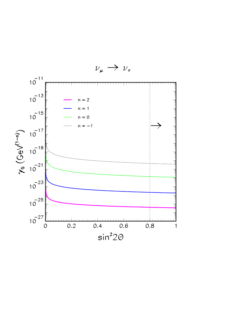
FIG. 2.: Limits on $\gamma_{0}$ as a function of $\sin^{2}2\theta$ in the $\nu_{\mu}\rightarrow\nu_{\tau}$ mode, for $n=-1,0,1$ and $2$. The excluded region at 99 % C.L. is the one to the right of each curve. The lower value of the amplitude consistent with the ANP is marked by a dashed line with an arrow. All the limits were obtained with CHORUS data.

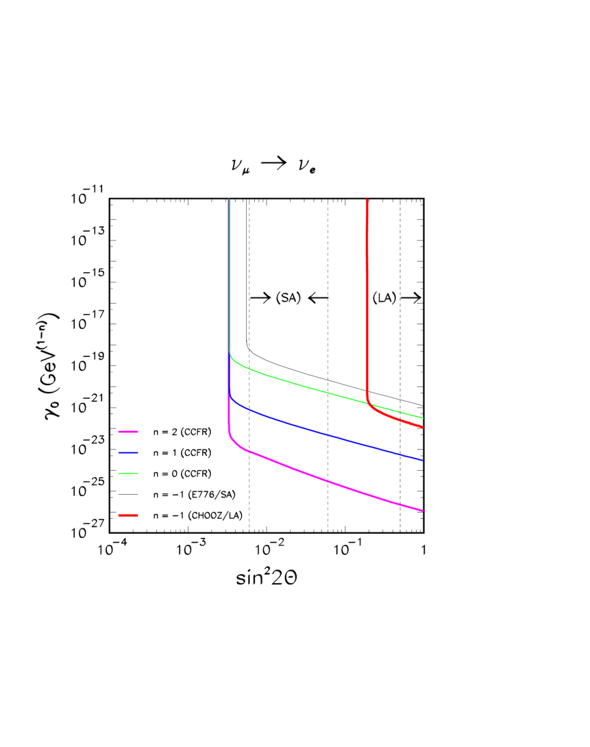
FIG. 3.: Limits on $\gamma_{0}$ as a function of $\sin^{2}2\theta$ in the $\nu_{\mu}\rightarrow\nu_{e}$ mode, for $n=-1$ (SA, LA), $0,1$ and $2$ at 99 % C.L.

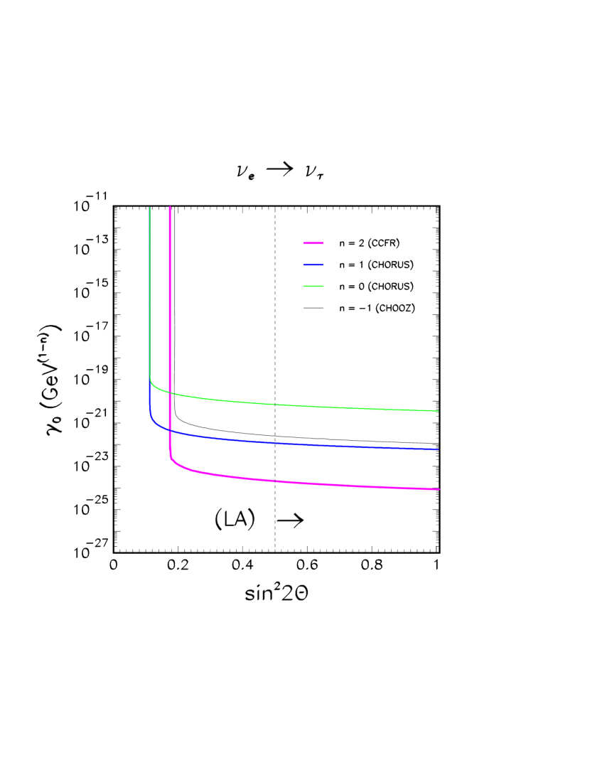
FIG. 4.: Limits on $\gamma_{0}$ as a function of $\sin^{2}2\theta$ in the $\nu_{e}\rightarrow\nu_{\tau}$ mode, for $n=-1,0,1$ and $2$ at 99 % C.L.

FIG. 5.: Limits on $\gamma_{0}$ for some of the next generation neutrino long baseline experiments assuming the proposed sensitivity of each experiment and no signal of oscillation observed in the $\nu_{\mu}\rightarrow\nu_{e}$ and $\nu_{e}\rightarrow\nu_{\tau}$ modes.

FIG. 6.: Attainable limits on $\gamma_{0}$ for some of the next generation neutrino long baseline experiments assuming they will observe neutrino oscillation.

- [1] Homestake Collaboration, K. Lande et al., Astrophys. J. 496, 505 (1998); GALLEX Collaboration, W. Hampel et al., Phys. Lett. B 447, 127 (1999); V. Gavrin for the SAGE Collaboration, talk given at the XIX International Conference on Neutrino Physics and Astrophysics (Neutrino 2000), Sudbury, Canada, June 16-21, 2000, available at http://nu2000.sno.laurentian.ca/V.Gavrin/index.html; E. Bellotti for the GNO Collaboration, talk given at the XIX International Conference on Neutrino Physics and Astrophysics (Neutrino 2000), Sudbury, Canada, June 16-21, 2000, available at http://nu2000.sno.laurentian.ca/E.Bellotti/index.html; Y. Suzuki for the Super-Kamiokande Collaboration, talk given at the XIX International Conference on Neutrino Physics and Astrophysics (Neutrino 2000), Sudbury, Canada, June 16-21, 2000, available at http://nu2000.sno.laurentian.ca/Y.Suzuki/index.html.
- [2] Kamiokande Collab., H. S. Hirata et al. Phys. Lett. B 205, 416 (1988); ibid. 280, 146 (1992); Y. Fukuda et al., ibid. B 335, 237 (1994); IMB Collab., R. Becker-Szendy et al. Phys. Rev. D 46, 3720 (1992); Super-Kamiokande Collab., Y. Fukuda et al. ibid. B 433, 9 (1998); ibid. B 436, 33 (1998); Phys. Rev. Lett. 81, 1562 (1998); T. Mann for the Soudan-2 Collaboration, talk given at the XIX International Conference on Neutrino Physics and Astrophysics (Neutrino 2000), Sudbury, Canada, June 16-21, 2000, available at http://nu2000.sno.laurentian.ca/T.Mann/index.html; B. Barish for the MACRO Collaboration, talk given at the XIX International Conference on Neutrino Physics and Astrophysics (Neutrino 2000), Sudbury, Canada, June 16-21, 2000, available at http://nu2000.sno.laurentian.ca/B.Barish/index.html; H. Sobel for the Super-Kamiokande Collaboration, talk given at the XIX International Conference on Neutrino Physics and Astrophysics (Neutrino 2000), Sudbury, Canada, June 16-21, 2000, available at http://nu2000.sno.laurentian.ca/H.Sobel/index.html.
- [3] S. Hawking, Phys. Rev. D, 14, 2460 (1975); Comm. Math. Phys. 43, 199 (1975).
- [4] S. Hawking, Comm. Math. Phys. 87, 395 (1982); Phys. Rev. D 37, 904 (1988); Phys. Rev. D 53, 3099 (1996); S. Hawking and C. Hunter, Phys. Rev. D 59, 044025 (1999).
- [5] F. Benatti and R. Floreanini, Phys. Lett. B 389, 100 (1996).
- [6] J. Ellis, J. S. Hagelin, D. V. Nanopoulos and M. Srednicki, Nucl. Phys. B 241, 381 (1984).
- [7] S. Coleman, Nucl. Phys. B 307, 867 (1988).
- [8] L. J. Garay, Phys. Rev. Lett. 80, 2508 (1998); Phys. Rev. D 58, 124015 (1998).
- [9] F. Benatti and R. Floreanini, JHEP 0002, 32 (2000).
- [10] J. Ellis, N. E. Mavromatos, and D. V. Nanopoulos, Phys. Lett. B 293, 142 (1992).
- [11] CPLEAR Collaboration, J. Ellis et al., Phys. Lett. B 364, 239 (1995).
- [12] P. Huet and M. E. Peskin, Nucl. Phys. B 434, 3 (1995).
- [13] F. Benatti and R. Floreanini, Phys. Lett. B 401, 337 (1997); F. Benatti and R. Floreanini, Nucl. Phys. B 488, 335 (1997); F. Benatti and R. Floreanini, Nucl. Phys. B 511, 550 (1998); F. Benatti and R. Floreanini, Phys. Lett. B 465, 260 (1999).
- [14] F. Benatti and R. Floreanini, Phys. Lett. B 451, 422 (1999).
- [15] Y. Liu, L. Hu, and M. Ge, Phys. Rev. D 56, 6648 (1997).
- [16] C.-H. Chang et al., Phys. Rev. D 60, 033006 (1999).
- [17] E. Lisi, A. Marrone, and D. Montanino, Phys. Rev. Lett. 85, 1166 (2000).
- [18] E. Lisi, talk given at the XIX International Conference on Neutrino Physics and Astrophysics (Neutrino 2000), Sudbury, Canada, June 16-21, 2000, available at http://nu2000.sno.laurentian.ca/E.Lisi/index.html.
- [19] A. M. Gago, H. Nunokawa and, R. Zukanovich Funchal, hep-ph/0007270, to be published in Phys. Rev. D.
- [20] M. C. Gonzalez-Garcia, talk given at the XIX International Conference on Neutrino Physics and Astrophysics (Neutrino 2000), Sudbury, Canada, June 16-21, 2000, available at http://nu2000.sno.laurentian.ca/M.Gonzalez-Garcia/index.html.
- [21] G. Mills for the LSND Collaboration, talk given at the XIX International Conference on Neutrino Physics and Astrophysics (Neutrino 2000), Sudbury, Canada, June 16-21, 2000, available at http://nu2000.sno.laurentian.ca/G.Mills/index.html.
- [22] K. Eitel for the KARMEN Collaboration, talk given at the XIX International Conference on Neutrino Physics and Astrophysics (Neutrino 2000), Sudbury, Canada, June 16-21, 2000, available at http://nu2000.sno.laurentian.ca/K.Eitel/index.html.
- [23] B. Achkar et al., Nucl. Phys. B 434, 503 (1995).
- [24] A. Romosan et al., Phys. Rev. Lett. 78, 2912 (1997); D. Naples et al., Phys, Rev. D 59, 031101 (1999).
- [25] L. Borodovsky et al., Phys. Rev. Lett. 68, 274 (1992).
- [26] E. Eskut et al., CERN-PPE/97-33, available at http://choruswww.cern.ch/Publications/papers.html/.
- [27] O. Sato, Nucl. Phys. (Proc. Suppl.) B 77, 220 (1999).
- [28] E. Radicioni, Nucl. Phys. (Proc. Suppl.) B 85, 95 (2000).
- [29] The CHORUS Collaboration,contributed paper to the XIX International Symposium on Lepton and Photon Interactions at High Energies, Stanford University, U.S.A., August 9-14, 1999, hep-ex/990715.
- [30] L. Ludovici for the CHORUS Collaboration, talk given at the XIX International Conference on Neutrino Physics and Astrophysics (Neutrino 2000), Sudbury, Canada, June 16-21, 2000, available at http://nu2000.sno.laurentian.ca/L.Ludovici/index.html.
- [31] M. Apollonio et al., Phys. Lett. B 466, 415 (1999).
- [32] E. B. Davies, Quantum Theory of Open Systems (Academic Press, New York, 1976); K. Kraus, States, Effects and Operations, Lect. Notes Phys. bf 190 (Springer Verlag, Berlin, 1983).
- [33] J. Pantaleone, T. K. Kuo, and S. W. Mansour, Phys. Rev. D 61, 033011 (2000).
- [34] The charged current cross sections for and can be obtained in form of a table from http://www.cern.ch/NGS.
- [35] S. Baker and R. Cousins, Nucl. Instrum. Methods. Phys. Res. 221, 434 (1984).
- [36] G. Feldman and R. D. Cousins, Phys. Rev. D 57, 3873 (1998).
- [37] R. D. Cousins and V. L. Highland, Nucl. Instr. and Meth. A320, 331 (1992).
- [38] Super-Kamiokande Collab., S. Fukuda et al., hep-ex/0009001.
- [39] L. Di Lella, in the Proceedings of the XIXth International Symposium on Lepton and Photon Interactions at High Energies, Stanford, CA, 1999, hep-ex/9912010.
- [40] A. Piepke for the KamLAND Collaboration, talk given at the XIX International Conference on Neutrino Physics and Astrophysics (Neutrino 2000), Sudbury, Canada, June 16-21, 2000, available at http://nu2000.sno.laurentian.ca/A.Piepke/index.html.
- [41] The MINOS Collaboration, “Neutrino Oscillation Physics at Fermilab: The NuMI-MINOS Project”, Fermilab Report No. NuMI-L-375 (1998).
- [42] The MINOS Collaboration, P. Adamson et al., Fermilab Report No. NuMI-L-337 (1998).
- [43] The MINOS Collaboration, K. R. Langenbach and M. C. Goodman, Fermilab Report No. NuMI-L-75 (1995).
- [44] A. Rubbia for the ICANOE/OPERA Collaboration, talk given at the XIX International Conference on Neutrino Physics and Astrophysics (Neutrino 2000), Sudbury, Canada, June 16-21, 2000, available at http://nu2000.sno.laurentian.ca/A.Rubbia/index.html.
- [45] ICANOE, A proposal for a CERN-GS long baseline and atmospheric neutrino oscillation experiment, INFN/AE-99-17, CERN/SPSC 99-25, SPSC/P314, August, 1999, see http://pcnometh4.cern.ch/publications.html.
- [46] S. Geer, Phys. Rev. D 57, 6989 (1998); Phys. Rev. D 59, 039903 (1999).
- [47] H. V. Klapdor-Kleingrothaus, H. Päs, and U. Sarkar, hep-ph/0004123.
- [48] A. Yu. Smirnov, D. N. Spergel, and J. N. Bahcall, Phys. Rev. D 49, 1389 (1994)