Abstract

We present analytical next-to-leading order results for the correlator of baryonic currents at the three-loop level with one finite mass quark. We obtain the massless and the HQET limits of the correlator as particular cases from the general formula, we also give explicit expressions for the moments of the spectral density. Calculations have been performed with an extensive use of the symbolic manipulation programs MATHEMATICA and REDUCE.

Prepared for the “VII International Workshop on Advanced Computing
and Analysis Techniques in Physics Research (ACAT2000)”

Baryons form a rich family of particles which has been experimentally studied with high accuracy [1]. A theoretical analysis of these experimental data gives a lot of information about the structure of QCD and the numerical values of its parameters. The hypothetical limit $N_{c}\to\infty$ for the number $N_{c}$ of colours which is a very powerful tool for investigating the general properties of gauge interactions was especially successful for baryons [2]. The spectrum of baryons is contained in the correlator of two baryonic currents and the spectral density associated with it. To leading order the correlator is given by a product of $N_{c}$ fermionic propagators. The diagrams of this topology have recently been studied in detail [3, 4, 5, 6, 7, 8]. They are rather frequently used in phenomenological applications [9]. With the advent of new accelerators and detectors many properties of baryons containing a heavy quark have been experimentally measured in recent years [1]. However, theoretical calculations beyond the leading order have not been done for many interesting cases. In this note we fill up this gap.

We report on the results of calculating the $\alpha_{s}$ corrections to the correlator of two baryonic currents with one finite mass quark and two massless quarks. We give analytical results and discuss the magnitude of the $\alpha_{s}$ corrections. The massless and HQET limits are obtained as special cases. We also present analytical results for the moments of the spectral density associated with the correlator. The extensive discussion of the impact of our new result for the correlator on the phenomenology of baryons will be given elsewhere. Note that the massless case has been known since long ago [10]. The mesonic analogue of our baryonic calculation was completed some time ago [11] and has subsequently provided a rich source of inspiration for many applications in meson physics.

A generic baryonic current has the form

$$j=\epsilon^{abc}(u_{a}^{T}Cd_{b})\Gamma\Psi_{c}$$ (1)

which has the quantum numbers of a $J^{P}=1/2^{-}$ baryon for $\Gamma=\gamma_{5}$. $\Psi$ is a finite mass quark field with the mass parameter $m$, $u$ and $d$ are massless quark fields, $C$ is the charge conjugation matrix, $\epsilon^{abc}$ is the totally antisymmetric tensor and $a,b,c$ are colour indices for the $SU(3)$ colour group. Other baryonic currents with any given specified quantum numbers are obtained from the current in Eq. (1) by inserting the appropriate Dirac matrices. Such additions introduce no principal complication into our method of calculation. In the following we take $\Gamma=1$. The correlator of two baryonic currents is expanded as

$$i\int\langle Tj(x)\bar{j}(0)\rangle e^{iqx}dx=\gamma_{\nu}q^{\nu}\Pi_{q}(q^{2})+m\Pi_{m}(q^{2}).$$ (2)

$\Gamma=\gamma_{5}$ leads to the trivial change $\Pi_{q}(q^{2})\to-\Pi_{q}(q^{2})$. The result for the invariant function $\Pi_{m}(q^{2})$ has already been presented in Ref. [12]. In this note we show results for the function $\Pi_{q}(q^{2})$ and compare it with $\Pi_{m}(q^{2})$. The invariant functions $\Pi_{q,m}(q^{2})$ can be represented compactly via the dispersion relation

$$\Pi_{\#}(q^{2})=\frac{1}{128\pi^{4}}\int_{m^{2}}^{\infty}\frac{\rho^{\#}(s)ds}{s-q^{2}}$$ (3)

where $\rho^{\#}(s)=\rho^{q,m}(s)$ are the spectral densities. All quantities are understood to be appropriately regularized. The spectral density is the real object of interest for phenomenological applications and we limit our subsequent discussion therefore to the spectral density

$$\rho^{\#}(s)=s^{2}\left\{\rho_{0}^{\#}(s)\left(1+\frac{\alpha_{s}}{\pi}\ln\left(\frac{\mu^{2}}{m^{2}}\right)\right)+\frac{\alpha_{s}}{\pi}\rho_{1}^{\#}(s)\right\}.$$ (4)

Here $\mu$ is the renormalization scale parameter, $m$ is a pole mass of the heavy quark (see e.g. Ref. [13]) and $\alpha_{s}=\alpha_{s}(\mu)$. The leading order two-loop contribution is shown in Fig. 1(a).

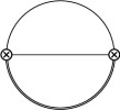
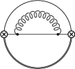
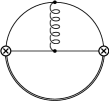
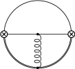
(a)(b)(c)(d)(e)

Figure 1: The calculated (a) two-loop and (b–e) three-loop topologies

Note that this topology coincides with water melon diagrams for which a general method of calculation (with arbitrary masses) has recently been developed [5, 6, 7]. The leading order results read

$$\rho_{0}^{q}(s)=\frac{1}{4}-2z+2z^{3}-\frac{1}{4}z^{4}-3z^{2}\ln z,$$ (5)

$$\rho_{0}^{m}(s)=1+9z-9z^{2}-z^{3}+6z(1+z)\ln z$$ (6)

with $z=m^{2}/s$. The next-to-leading order contribution is given by three-loop diagrams with one external momentum. For an arbitrary mass arrangement such diagrams have not yet been calculated analytically. However, if we take the case of one massive line, the result within $\overline{\rm MS}$-scheme can be obtained analytically and reads

$$\rho_{1}^{q}(s)\ =\ \frac{71}{48}-\frac{565}{36}z-\frac{7}{8}z^{2}+\frac{625}{36}z^{3}-\frac{109}{48}z^{4}$$

$$\kern-14.0pt-\left(\frac{49}{36}-\frac{116}{9}z+\frac{116}{9}z^{3}-\frac{49}{36}z^{4}\right)\ln(1-z)+\left(\frac{1}{4}-\frac{17}{3}z-11z^{2}+\frac{113}{9}z^{3}-\frac{49}{36}z^{4}\right)\ln z$$

$$\kern-14.0pt+\left(\frac{1}{3}-\frac{8}{3}z+\frac{8}{3}z^{3}-\frac{1}{3}z^{4}\right)\ln(1-z)\ln z-2z^{2}\left(9+\frac{4}{3}z-\frac{1}{6}z^{2}\right)\left(\frac{1}{2}\ln^{2}z-\zeta(2)\right)$$

$$\kern-14.0pt+\left(\frac{2}{3}-\frac{16}{3}z-18z^{2}+\frac{8}{3}z^{3}-\frac{1}{3}z^{4}\right){\rm Li}_{2}(z)-12z^{2}\left({\rm Li}_{3}(z)-\zeta(3)-\frac{1}{3}{\rm Li}_{2}(z)\ln(z)\right)$$

where ${\rm Li}_{n}(z)$ are polylogarithms and $\zeta(n)$ is Riemann’s zeta function, $\zeta(2)=\pi^{2}/6$. The contributing three-loop diagrams are shown in Figs. 1(b) to (e). They have been evaluated using advanced algebraic methods for multi-loop calculations along the lines decribed in Refs. [6, 11]. This result should be compared to

$$\rho_{1}^{m}(s)\ =\ 9+\frac{665}{9}z-\frac{665}{9}z^{2}-9z^{3}$$

$$-\left(\frac{58}{9}+42z-42z^{2}-\frac{58}{9}z^{3}\right)\ln(1-z)+\left(2+\frac{154}{3}z-\frac{22}{3}z^{2}-\frac{58}{9}z^{3}\right)\ln z$$

$$+4\left(\frac{1}{3}+3z-3z^{2}-\frac{1}{3}z^{3}\right)\ln(1-z)\ln z+12z\left(2+3z+\frac{1}{9}z^{2}\right)\left(\frac{1}{2}\ln^{2}z-\zeta(2)\right)$$

$$+4\left(\frac{2}{3}+12z+3z^{2}-\frac{1}{3}z^{3}\right){\rm Li}_{2}(z)+24z(1+z)\left({\rm Li}_{3}(z)-\zeta(3)-\frac{1}{3}{\rm Li}_{2}(z)\ln z\right).$$

Our method of integration is a completely algebraic one and therefore symbolic manipulation programs can be used for performing the long calculations. Two independent calculations of some steps were done using REDUCE and MATHEMATICA. REDUCE is rather actively used for high energy calculations (see e.g. Ref. [14]). All diagrams have first been reduced to scalar prototypes. The integrals over massless loops have been performed (for recurrent integration where possible) and one is left with the basic integral

$$V(\alpha,\beta;q^{2}/m^{2})=\int\frac{d^{D}k}{(k^{2}+m^{2})^{\alpha}(q-k)^{2\beta}}$$ (9)

which is a generalization of the standard object $G(\alpha,\beta)$ of the massless calculation [15, 16]. The integral $V$ is known analytically and it suffices in order to calculate the diagrams in Figs. 1(c) and (d). For the calculation of the diagram shown in Fig. 1(e) the basic integral $V$ enters as a subdiagram. This subdiagram then is represented in terms of a dispersion integral which makes the whole diagram computable in terms of the same $V$ with the argument depending on the loop momentum. The final step is a finite range (convolution type) integration over this internal momentum with a spectral density of the basic integral $V$. The reduction to scalar prototypes of the diagram shown in Fig. 1(e) leads also to a new irreducible block (i.e. a prototype not expressible in terms of $V$) which is related to a two-loop master (fish) diagram. The result for this diagram is taken from Ref. [17].

The results given in Eqs. (S0.Ex3) and (S0.Ex6) represent the full next-to-leading order solution. Since the anomalous dimension of the current in Eq. (1) is known up to two-loop order [18], the results shown in Eqs. (S0.Ex3) and (S0.Ex6) complete the ingredients necessary for an analysis of the correlator in Eq. (2) within operator product expansion at the next-to-leading order level.

We now turn to the analysis of Eq. (S0.Ex3) and contrast it with the corresponding results for $\rho^{m}(s)$ as published in Ref. [12]. Two limiting cases of general interest are the near-threshold and the high energy asymptotics. With our result given in Eq. (S0.Ex3) both limits can be taken explicitly. The asymptotic expressions can be also obtained in the framework of effective theories which can be viewed as special devices for such calculations.

In the high energy (or, equivalently, small mass) limit $z\rightarrow 0$ the corrections read

$$\rho_{1}^{q}(s) = \frac{71}{48}+\frac{1}{4}\ln z-\frac{41}{3}z-6z\ln z+O(z^{2}),$$ (10)

$$\rho_{1}^{m}(s) = 9+83z-4\pi^{2}z+2\ln z+50z\ln z+12z\ln^{2}z-24z\zeta(3)+O(z^{2}).\qquad$$ (11)

Therefore we obtain

$$\rho^{q}(s)\ =\ \rho_{\rm massless}^{q}(s)$$

$$= \frac{s^{2}}{4}\left\{1+\frac{\alpha_{s}}{\pi}\left(\ln\left(\frac{\mu^{2}}{s}\right)+\frac{71}{12}\right)\right\}-2m_{\overline{\rm MS}}^{2}(\mu)s\left\{1+\frac{\alpha_{s}}{\pi}\left(3\ln\left(\frac{\mu^{2}}{s}\right)+\frac{19}{2}\right)\right\},$$

$$m\rho^{m}(s)\ =\ m_{\overline{\rm MS}}(\mu)\rho_{\rm massless}^{m}(s)\ =\ m_{\overline{\rm MS}}(\mu)s^{2}\left\{1+\frac{\alpha_{s}}{\pi}\left(2\ln\left(\frac{\mu^{2}}{s}\right)+\frac{31}{3}\right)\right\}$$ (13)

where $\rho_{\rm massless}^{\#}(s)$ is the result of calculating the correlator in the effective theory of massless quarks. For the momentum part $\rho^{q}(s)$ we retain the $O(m^{2})$ correction. The relation between the pole mass $m$ and the $\overline{\rm MS}$ mass $m_{\overline{\rm MS}}(\mu)$ we have used reads

$$m=m_{\overline{\rm MS}}(\mu)\left\{1+\frac{\alpha_{s}}{\pi}\left(\ln\left(\frac{\mu^{2}}{m^{2}}\right)+\frac{4}{3}\right)\right\}.$$ (14)

Note that the massless effective theory cannot reproduce the mass singularities (terms like $z\ln(z)$ in Eq. (11)). These singularities can be parametrized by condensates of local operators. The first $m^{2}$ correction in Eqs. (6) and (11) (or, equivalently, the $m^{3}$ correction to the expression in Eq. (13)) can be found if the perturbative value of the heavy quark condensate $\langle 0|\bar{\Psi}\Psi|0\rangle$ taken from the full theory is added [19]. The composite operator $(\bar{\Psi}\Psi)$ should be understood within a mass independent renormalization scheme such as the $\overline{\rm MS}$-scheme. This value (perturbatively, $\langle 0|\bar{\Psi}\Psi|0\rangle\sim m^{3}\ln(\mu^{2}/m^{2})$) cannot be computed within the effective theory of massless quarks. It provides the proper matching between the perturbative expressions for the correlators of the full (massive) and effective (massless) theories. This matching procedure allows one to restore higher order terms of the mass expansion in the full theory from the effective massless theory with the mass term treated as a perturbation [20]. The account for the mass term as a perturbation in a massless theory is justified at high energies and greatly simplifies the calculations (see e.g. Ref. [21]). Note that the correction of order $m^{2}/s$ to $\rho^{m}(s)$ can actually be found in this manner because it depends only on one local operator $(\bar{\Psi}\Psi)$ and, therefore, the calculation is technically feasible. In case of the function $\rho^{q}(s)$ the situation is different because there is no gauge invariant operator of dimension two in the effective massless theory. Therefore, the mass singularities of the form $m^{2}\log(m^{2}/s)$ should not appear in the expansion for $\rho^{q}(s)$ at large energies. The result in Eq. (S0.Ex7) shows this explicitly. Note that the absence of such singularities is one of our checks of the correctness of the calculation.

In the near-threshold limit $E\rightarrow 0$ with $s=(m+E)^{2}$ one explicitly obtains

$$\rho_{\rm thr}^{m}(m,E) = \frac{16E^{5}}{5m}\Bigg{\{}1+\frac{\alpha_{s}}{\pi}\ln\left(\frac{\mu^{2}}{m^{2}}\right)$$

$$\qquad\qquad+\frac{\alpha_{s}}{\pi}\left(\frac{54}{5}+\frac{4\pi^{2}}{9}+4\ln\left(\frac{m}{2E}\right)\right)\Bigg{\}}+O\left(\frac{E^{6}}{m^{2}}\right).$$

The invariant function $\rho^{m}(s)$ suffices to determine the complete leading HQET behaviour since one has $q\kern-5.5pt/\rho^{q}+m\rho^{m}\rightarrow(v\kern-5.0pt\raise 1.0pt\hbox{$\scriptstyle/$}\kern 1.0pt+1)\rho_{\rm HQET}$ for the leading term. We explictly checked this relation. In this region the appropriate device to compute the limit of the correlator is HQET (see e.g. Refs. [22, 23]). Writing

$$m\rho_{\rm thr}^{m}(m,E)=C(m/\mu,\alpha_{s})^{2}\rho_{\rm HQET}(E,\mu)$$ (16)

we obtain the known result for $\rho_{\rm HQET}(E,\mu)$ [24]

$$\rho_{\rm HQET}(E,\mu)=\frac{16E^{5}}{5}\left\{1+\frac{\alpha_{s}}{\pi}\left(\frac{182}{15}+\frac{4\pi^{2}}{9}+4\ln\frac{\mu}{2E}\right)\right\}+O(E^{6})$$ (17)

with the matching coefficient $C(m/\mu,\alpha_{s})$ given by [25]

$$C(m/\mu,\alpha_{s})=1+\frac{\alpha_{s}}{\pi}\left(\frac{1}{2}\ln\left(\frac{m^{2}}{\mu^{2}}\right)-\frac{2}{3}\right).$$ (18)

The matching procedure allows one to restore the near-threshold limit of the full correlator starting from the simpler effective theory near the threshold [26].

Note that the higher order corrections in $E/m$ to Eq. (S0.Ex8) can easily be obtained from the explicit result given in Eq. (S0.Ex3). Indeed, the next-to-leading order corrections in low energy expansion read

$$\Delta\rho_{\rm thr}^{q}(m,E) = -\frac{8E^{6}}{m^{2}}\Bigg{\{}1+\frac{\alpha_{s}}{\pi}\left(\ln\left(\frac{\mu^{2}}{m^{2}}\right)+\frac{908}{75}+\frac{4\pi^{2}}{9}+\frac{68}{15}\ln\left(\frac{m}{2E}\right)\right)\Bigg{\}},$$ (19)

$$\Delta\rho_{\rm thr}^{m}(m,E) = -\frac{24E^{6}}{5m^{2}}\left\{1+\frac{\alpha_{s}}{\pi}\left(\ln\left(\frac{\mu^{2}}{m^{2}}\right)+\frac{584}{45}+\frac{4\pi^{2}}{9}+\frac{44}{9}\ln\left(\frac{m}{2E}\right)\right)\right\}.\qquad$$ (20)

To obtain this result starting from HQET is a more difficult task requiring the analysis of contributions of higher dimension operators.

Figure 2: The ratio $\rho_{1}^{m}(s)/\rho_{0}^{m}(s)$ of the next-to-leading correction and the leading order term in dependence of the energy square $s$

We now discuss some quantitative features of the correction given in Eq. (S0.Ex3). Of interest is whether the two limiting expressions (the massless limit expression as given in Eq. (S0.Ex7) and the HQET limit expression in Eqs. (S0.Ex8) and (16)) can be used to characterise the full function for all energies.

For this discussion we compare components of the baryonic spectral function in leading and next-to-leading order. In Fig. 2 and 3 we show the ratio $\rho_{1}^{\#}(s)/\rho_{0}^{\#}(s)$ for $\#=m$ and $\#=q$, respectively. In the following we shall always use the specific renormalization scale value $\mu=m$ if it is not written explicitly.

Figure 3: The ratio $\rho_{1}^{q}(s)/\rho_{0}^{q}(s)$ of the next-to-leading correction and the leading order term in dependence of the energy square $s$

One can see that a simple interpolation between the two limits can give a rather good approximation for the next-to-leading order correction in the complete region of $s$.

The informative set of observables are moments of the spectral density

$${\cal M}_{n}^{\#}=\int_{m^{2}}^{\infty}\frac{\rho^{\#}(s)ds}{s^{n}}=m^{6-2n}M_{n}^{\#}$$ (21)

where $M_{n}^{\#}$ are dimensionless quantities. We find

$$M_{n}^{\#}=M_{n}^{\#{(0)}}\left\{1+\frac{\alpha_{s}}{\pi}\left(\ln\left(\frac{\mu^{2}}{m^{2}}\right)+\delta_{n}^{\#}\right)\right\}$$ (22)

where

$$M_{n}^{q(0)} = \frac{12}{(n+1)n(n-1)^{2}(n-2)(n-3)},$$ (23)

$$M_{n}^{m(0)} = \frac{12}{n(n-1)^{2}(n-2)^{2}(n-3)},$$ (24)

and

$$\delta_{n}^{\#}=A_{n}^{\#}+\frac{2\pi^{2}}{9}.$$ (25)

The coefficients $A_{n}^{\#}$ are rational numbers, and the closed form expressions for $\delta_{n}^{\#}$ are long. Therefore we only show the first values for $A_{n}^{q}$ in the second column of Table 1. They are numerically rather close to the results obtained for $A_{n}^{m}$ in Ref. [12].

$n$	$A^{q}_{n}$	$\delta^{q}_{n}-\delta^{q}_{n-1}$
$4$	$9/2$
$5$	$22/3$	$2.833333$
$6$	$109/12$	$1.750000$
$7$	$5593/540$	$1.274074$
$8$	$6133/540$	$1.000000$
$9$	$460351/37800$	$0.821190$
$10$	$40553/3150$	$0.695370$
$11$	$148574/11025$	$0.602132$
$12$	$2470739/176400$	$0.530357$
$13$	$758614613/52390800$	$0.473463$
$14$	$156200257/10478160$	$0.427302$
$15$	$4583939335/299675376$	$0.389128$
$16$	$117273501721/7491884400$	$0.357055$
$17$	$3113341968041/194788994400$	$0.329746$
$18$	$3172990981751/194788994400$	$0.306224$
$19$	$54887116886639/3311412904800$	$0.285760$
$20$	$111547839702373/6622825809600$	$0.267802$
$21$	$7313770708819951/427834547300160$	$0.251920$
$22$	$1483100149208267/85566909460032$	$0.237779$
$23$	$142724395992842749/8128856398703040$	$0.225109$

Table 1: Values for the rational part $A^{q}_{n}$ of the first moments $\delta^{q}_{n}$ and their relative difference $\delta^{q}_{n}-\delta^{q}_{n-1}$

By representing the moments through

$$\frac{M_{n}^{\#}}{M_{n}^{\#(0)}}=\frac{M_{N}^{\#}}{M_{N}^{\#(0)}}\left\{1+\frac{\alpha_{s}}{\pi}(\delta_{n}^{\#}-\delta_{N}^{\#})\right\}$$ (26)

we have all corrections to be normalized to the moment $M_{N}^{\#}$ of fixed order $N$. Note that the difference $\delta_{n}^{\#}-\delta_{N}^{\#}$ is scheme-independent. This feature can be used in the high precision analysis of heavy quark properties [27] within NRQCD (see e.g. Ref. [28]). With Eq. (26) one can find the actual (invariant or scheme-independent) magnitude of the correction. Indeed, for any given $N$ one can find a set of perturbatively commensurate moments $M_{n}^{\#}$ with $n\sim N$ for which the requirement of the chosen precision is satisfied. In the third column of Table 1 we therefore present numerical values only for the differences of the $\delta_{n}^{q}$ for subsequent orders.

Note that the moments represent massive vacuum bubbles, i.e. diagrams with massive lines without external momenta. These diagrams have been comprehensively analyzed in Refs. [29, 30]. The analytical results for the first few moments at three-loop level can be checked independently with existing computer programs for symbolic calculations in high energy physics (see e.g. Ref. [31]).

The presented results have phenomenological applications within the sum rule analysis of baryon properties (see e.g. Refs. [32, 33, 34]). As an example we calculate the integral of $\rho^{q}(s)$ up to the energy cut $\sqrt{s_{0}}$,

$${\cal M}_{0}^{q}(s_{0})=\int_{m^{2}}^{s_{0}}\rho^{q}(s)ds$$ (27)

which is related to the coupling constant (residue) of a baryon to the current in Eq. (1). In NLO the integral is represented by

$${\cal M}_{0}^{q}(s_{0})={\cal M}_{0}^{q(0)}(s_{0})\left(1+\frac{\alpha_{s}}{\pi}\left(\ln\left(\frac{\mu^{2}}{m^{2}}\right)+\Delta(s_{0})\right)\right)$$ (28)

which leads to the renormalization of the LO result for the residue in the form

$$Z_{R}^{01}=\frac{{\cal M}_{0}^{q}(s_{0})}{{\cal M}_{0}^{q(0)}(s_{0})}=1+\frac{\alpha_{s}}{\pi}\left(\ln\left(\frac{\mu^{2}}{m^{2}}\right)+\Delta(s_{0})\right)+O(\alpha_{s}^{2}).$$ (29)

For e.g. $s_{0}=2m^{2}$, $\mu^{2}=m^{2}$ we find numerically

$$Z_{R}^{01}=1+\frac{\alpha_{s}}{\pi}\Delta(2m^{2})=1+\frac{\alpha_{s}}{\pi}15.4117\ldots$$ (30)

We see that the NLO correction to the residue in the $\overline{\rm MS}$-scheme is rather large. For the numerical value of the coupling constant $\alpha_{s}\approx 0.3$ which is a typical value for baryons containing a $c$-quark, the NLO correction in the $\overline{\rm MS}$-scheme reaches the $100\%$ level.

One can see that the corrections to the moments basically reflect the shape of the correction to the spectrum. Even the massless approximation is reasonably good for relative corrections for the first few moments despite of the unfavorable shape of the weight function $1/s^{n}$. It can be improved by changing the subtraction point $\mu$, i.e. by switching from the $\overline{\rm MS}$-scheme to some other renormalization scheme, or by resumming the integrand [35] which lies beyond the scope of finite order perturbation theory though.

To conclude, we have computed the next-to-leading perturbative corrections to the finite mass baryon correlator at three-loop order. Technically, the method allows one to obtain analytical results for two-point correlators of composite operators with one finite mass particle that can be compared to HQET results. Corrections in $E/m$ near threshold are easily available from our explicit results. From threshold to high energies the exact spectral density interpolates nicely between the leading order HQET result close to threshold and the asymptotic mass zero result. Going even one order higher it is very likely that the full four-loop spectral density can be well approximated by the corresponding massless four-loop result which can be calculated using existing computational algorithms [36, 37].

Acknowledgements: The present work is supported in part by the Volkswagen Foundation under contract No. I/73611 and by the Russian Fund for Basic Research under contract 99-01-00091. A.A. Pivovarov is an Alexander von Humboldt fellow. S. Groote gratefully acknowledges a grant given by the DFG, FRG.

References

- [1] Particle Data Group, Eur. Phys. J. C3 (1998) 1
- [2] E. Witten, Nucl. Phys. B160 (1979) 57
- [3] F.A. Berends, A.I. Davydychev, N.I. Ussyukina, Phys. Lett. 426 B (1998) 95
- [4] S. Groote, J.G. Körner and A.A. Pivovarov, Phys. Rev. D60 (1999) 061701
- [5] S. Groote, J. G. Körner and A. A. Pivovarov, Eur. Phys. J. C11 (1999) 279
- [6] S. Groote, J. G. Körner and A. A. Pivovarov, Nucl. Phys. B542 (1999) 515
- [7] S. Groote, J. G. Körner and A. A. Pivovarov, Phys. Lett. 443 B (1998) 269
-
[8]
S. Groote and A.A. Pivovarov,
Nucl. Phys. B580 (2000) 459;
A.I. Davydychev and V.A. Smirnov, Nucl. Phys. B554 (1999) 391;
N.E. Ligterink, Phys. Rev. D61 (2000) 105010 -
[9]
J.O. Andersen, E. Braaten, M. Strickland,
Phys. Rev. D62 (2000) 045004;
S. Narison and A.A. Pivovarov, Phys. Lett. 327 B (1994) 341;
T. Sakai, K. Shimizu and K. Yazaki, Prog. Theor. Phys. Suppl. 137 (2000) 121;
S.A. Larin et al., Sov. J. Nucl. Phys. 44 (1986) 690;
J.M. Chung and B.K. Chung, Phys. Rev. D60 (1999) 105001;
K. Chetyrkin and S. Narison, Phys. Lett. 485 B (2000) 145;
H.Y. Jin and J.G. Körner, “Radiative correction of the correlator for () light hybrid currents”, Report No. MZ-TH/00-11, hep-ph/0003202 -
[10]
A.A. Ovchinnikov, A.A. Pivovarov and L.R. Surguladze,
Sov. J. Nucl. Phys. 48 (1988) 358; Int. J. Mod. Phys. A6 (1991) 2025 -
[11]
S.C. Generalis, Report No. OUT-4102-13 (1984),
later published as J. Phys. G16 (1990) 367, see also
D.J. Broadhurst, Phys. Lett. 101 B (1981) 423;
D.J. Broadhurst and S.C. Generalis, Report No. OUT-4102-8/R (1982) - [12] S. Groote, J.G. Körner and A.A. Pivovarov, Phys. Rev. D61 (2000) 071501(R)
- [13] R. Tarrach, Nucl. Phys. B183 (1981) 384
- [14] A.A. Pivovarov, Proceedings of the Conference “Pisa AIHENP 1995”, p. 301–306 [hep-ph/9505316]
- [15] G. Chetyrkin, A.L. Kataev and F.V. Tkachev, Nucl. Phys. B174 (1980) 345
-
[16]
K.G. Chetyrkin and F.V. Tkachov,
Nucl. Phys. B192 (1981) 159;
F.V. Tkachov, Phys. Lett. 100 B (1981) 65 - [17] D.J. Broadhurst, Z. Phys. C47 (1990) 115
-
[18]
A.A. Pivovarov and L.R. Surguladze,
Yad. Fiz. 48 (1988) 1856
[Sov. J. Nucl. Phys. 48 (1989) 1117]; Nucl. Phys. B360 (1991) 97 - [19] H.D. Politzer, Nucl Phys. B117 (1976) 397
- [20] V.P. Spiridonov and K.G. Chetyrkin, Sov. J. Nucl. Phys. 47 (1988) 522
- [21] K.G. Chetyrkin, J.H.Kühn, A. Kwiatkowski, Phys. Rept. 277 (1996) 189
- [22] H. Georgi, Nucl. Phys. B363 (1991) 301
- [23] M. Neubert, Phys. Rept. 245 (1994) 259
- [24] S. Groote, J.G. Körner and O.I. Yakovlev, Phys. Rev. D55 (1997) 3016
- [25] A.G. Grozin and O.I. Yakovlev, Phys. Lett. 285 B (1992) 254
- [26] E. Eichten and B. Hill, Phys. Lett. 234 B (1990) 511
-
[27]
A.A. Penin and A.A. Pivovarov,
Phys. Lett. 435 B (1998) 413;
Phys. Lett. 443 B (1998) 264; Nucl. Phys. B549 (1999) 217 - [28] A. Hoang et al., Eur. Phys. J. direct C3 (2000) 1
- [29] L.V. Avdeev, Comput. Phys. Commun. 98 (1996) 15
- [30] D.J. Broadhurst, Eur. Phys. J. C8 (1999) 311
- [31] K.G. Chetyrkin, J.H. Kühn and M. Steinhauser, Nucl. Phys. B505 (1997) 40
- [32] B.L. Ioffe, Nucl. Phys. B188 (1981) 317
- [33] Y. Chung et al., Phys. Lett. 102 B (1981) 175
-
[34]
N.V. Krasnikov, A.A. Pivovarov and N.N. Tavkhelidze,
JETP Lett. 36 (1982) 333; Z. Phys. C19 (1983) 301 -
[35]
A.A. Pivovarov, Sov. J. Nucl. Phys. 54 (1991) 676;
Z. Phys. C53 (1992) 461; Nuovo Cim. 105 A (1992) 813 -
[36]
K.G. Chetyrkin and F.V. Tkachov,
Nucl. Phys. B192 (1981) 159;
F.V. Tkachov, Phys. Lett. 100 B (1981) 65 - [37] K.G. Chetyrkin and V.A. Smirnov, Phys. Lett. 144 B (1984) 419