Cosmic Ray Air Shower Characteristics
in the Framework of the
Parton-Based Gribov-Regge Model NEXUS

Abstract

The purpose of this paper is twofold: first we want to introduce a new type of hadronic interaction model (neXus), which has a much more solid theoretical basis as, for example, presently used models like qgsjet and venus, and ensures therefore a much more reliable extrapolation towards high energies. Secondly, we want to promote an extensive air shower (EAS) calculation scheme, based on cascade equations rather than explicit Monte Carlo simulations, which is very accurate in calculations of main EAS characteristics and extremely fast concerning computing time. We employ the neXus model to provide the necessary data on particle production in hadron-air collisions and present the average EAS characteristics for energies $10^{14}-10^{17}$ eV. The experimental data of the casa-blanka group are analyzed in the framework of the new model.

1 Introduction

Although cosmic rays have been studied for many decades, there remain still many open questions, in particular concerning the high energy cosmic rays above $10^{14}$ eV. One does neither know their composition nor the sources and acceleration mechanisms, partly because of the fact that at these high energies direct measurements are impossible due to the weak flux. But since cosmic ray particles initiate cascades of secondaries in the atmosphere, the so-called extensive air showers, one may reconstruct cosmic ray primaries by measuring shower characteristics. This reconstruction requires, however, reliable model predictions for the simulation of EAS initiated by either protons or nuclei from helium to iron. The problem is that the energy of the cosmic rays may exceed by far the energy range accessible by modern colliders, where at most equivalent fixed target energies of roughly $10^{15}$ eV can be reached. The projects of new generation EAS arrays are aimed even to the energy region $10^{20}\div 10^{21}$ eV, and so the gap between the existing energy limit of collider data and the demands of cosmic ray experiments is considerable. Moreover, the real reliable data limits are essentially less than above mentioned, because at present time collider experiments do not register particles going into the extreme forward direction and a number of other drawbacks may be listed. Therefore there exists a real need of “reasonable” models, implementing the correct physics, in order to be able to make extrapolations towards extremely high energies.

Concerning models one has to distinguish between EAS models and hadronic interaction models. The latter ones like venus [1], qgsjet [2, 3], and sybill [4] are modeling hadron-hadron, hadron-nucleus and nucleus-nucleus collisions at high energies, being more or less sophisticated concerning the theoretical input, and relying in any case strongly on data from accelerator experiments. The EAS models like corsika [5] are actually simulating the full cascade of secondaries, using one of the above-mentioned hadronic models for the hadronic interactions and treating the well known electro-magnetic part of the shower. It turns out that the model predictions of EAS simulations depend substantially on the choice of the hadronic interaction model. In corsika, the average electron number in EAS at primary energy $10^{15}$ eV varies from $1.11\cdot 10^{5}$ to $1.62\cdot 10^{5}$ (at sea level) depending on the hadronic interaction model [6]. So the right choice of the model and its parameters is extremely important.

Recently a new hadronic interaction model neXus [7] has been proposed. It is characterized by a consistent treatment for calculating cross sections and particle production, considering energy conservation strictly in both cases (which is not the case in all above-mentioned models!). In addition, one introduces hard processes in a natural way, avoiding any unphysical dependence on artificial cutoff parameters. A single set of parameters is sufficient to fit many basic spectra in proton-proton and lepton-nucleon scattering, as well as in electron-positron annihilation. Briefly: concerning theoretical consistency, neXus is considerably superior to the presently used approaches, and allows a much safer extrapolation to very high energies.

This new approach cures some of the main deficiencies of two of the standard procedures currently used: the Gribov-Regge theory and the eikonalized parton model, the theoretical basis of the above-mentioned interaction models. There, cross section calculations and particle production cannot be treated in a consistent way using a common formalism. In particular, energy conservation is taken care of in case of particle production, but not concerning cross section calculations. In addition, hard contributions depend crucially on some cutoff and diverge for the cutoff being zero.

Having a reliable hadronic interaction model, one may now proceed to do air shower calculations. It may appear that an ideal solution from the user’s point of view is to use direct Monte Carlo technique, where the cascade is traced from the initial energy to the threshold one and the threshold energy corresponds to the minimum energy registered by the array in question. But such an approach takes unreasonably much computer time and sometimes gives no possibility to analyze experimental data in the appropriate way. Already at $10^{14}$ eV to $3\cdot 10^{16}$ eV, the experimental statistics from the kascade experiment [8] is ten times bigger than the corresponding number of simulated events. It should be mentioned that at higher energies (above $10^{17}$ eV) it is hardly possible to use direct Monte Carlo calculations. Of course, some modifications, like the thinning method [9], are possible and average values may be computed.

In this paper, we follow an alternative approach, where one treats the air shower development in terms of cascade equations. Here, the cascade evolution is characterized by differential energy spectra of hadrons, which one obtains by solving a system of integro-differential equations. Crucial input for these equations is the inclusive spectra of hadrons produced in hadron-air collisions. These spectra are obtained by performing neXus simulations and finally parameterizing the results. Having solved the cascade equations, we finally analyse the results of the casa-blanka group as a first application of our approach.

2 The NEXUS Model

The most sophisticated approach to high energy hadronic interactions is the so-called Gribov-Regge theory [10, 11]. This is an effective field theory, which allows multiple interactions to happen “in parallel”, with phenomenological object called “Pomerons” representing elementary interactions [12]. Using the general rules of field theory, one may express cross sections in terms of a couple of parameters characterizing the Pomeron. Interference terms are crucial, they assure the unitarity of the theory.

A big disadvantage is the fact that cross sections and particle production are not calculated consistently: the fact that energy needs to be shared between many Pomerons in case of multiple scattering is well taken into account when considering particle production (in particular in Monte Carlo applications), but not for cross sections [13].

Another problem is the fact that at high energies, one also needs a consistent approach to include both soft and hard processes. The latter ones are usually treated in the framework of the parton model, which only allows to calculate inclusive cross sections.

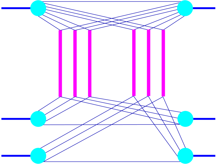
Figure 1: The diagram representing a proton-nucleus collision, or more precisely a proton interacting with (for simplicity) two target nucleons, taking into account energy conservation. Here, the energy of the incoming proton is shared between all the constituents, which provide the energy for interacting with two target nucleons.

We recently presented a completely new approach [14, 15, 7] for hadronic interactions and the initial stage of nuclear collisions, which is able to solve several of the above-mentioned problems. We provide a rigorous treatment of the multiple scattering aspect, such that questions of energy conservation are clearly determined by the rules of field theory, both for cross section and particle production calculations. In both (!) cases, energy is properly shared between the different interactions happening in parallel, see fig. 1 for hadron-nucleus collisions. This is the most important and new aspect of our approach, which we consider a first necessary step to construct a consistent model for high energy nuclear scattering.

The elementary diagram, shown as the thick lines in the above diagrams, is the sum of the usual soft Pomeron and the so-called semi-hard Pomeron, where the latter one may be obtained from perturbative QCD calculations (parton ladders). To some extent, our approach provides a link between the Gribov-Regge approach and the parton model, we call it “Parton-based Gribov-Regge Theory”.

3 System of Hadronic Cascade Equations

EAS are produced as a result of the hadronic cascade development in the atmosphere. We characterize hadronic cascades by the differential spectra $h_{n}(E,X)$ of hadrons of type $n$ with energy $E$ at an atmospheric depth $X$, the latter one being the integral over the atmospheric density $\rho$ along a straight line trajectory (not necessary radial) from some point $P$ to infinity,

$$X=\int_{P}^{\infty}\,\rho(x)dx,$$ (1)

measured usually in $\mathrm{g}/\mathrm{cm}^{2}$. The decrease of the average hadron numbers due to collisions with air nuclei is given as

$$\frac{dh_{n}}{dX}=-\frac{h_{n}}{\lambda_{n}},$$ (2)

where the mean inelastic free path $\lambda_{n}$ (in units of mass/area) can be expressed via the average hadron-air cross-section $\sigma_{\mathrm{inel}}^{(n)}$ and the average mass of air molecules $m_{air}$ :

$$\lambda_{n}=\frac{m_{\mathrm{air}}}{\sigma^{(n)}_{\mathrm{inel}}}$$ (3)

The second process to be considered is particle decay. The decay rate in the particle c.m. system is $dh_{n}/d\tau=-h_{n}/\tau_{0}$, with $\tau_{0}$ being the particle life time. For a relativistic particle we find

$$\frac{dh_{n}}{dX}=-\frac{B_{n}}{EX}h_{n},$$ (4)

with the decay constant in energy units

$$B_{n}=\frac{m_{n}}{\alpha c\tau_{0}},$$ (5)

where $m_{n}$ is the hadron mass and $c$ the velocity of light. The ratio $\alpha=\rho/X$ depends only weakly on $X$ and is for the following taken to be constant, which implies constant $B_{n}$. If we take the simple exponential barometric formula for the density $\rho$, we get

$$\alpha=\frac{\rho_{0}\,g\,\cos\theta}{P_{0}},$$ (6)

where $\rho_{0}$ and $P_{0}$ are density and pressure at (for example) sea level, $g$ the gravitational acceleration of the earth, and $\theta$ the zenith angle of the shower trajectory. In this paper, we only consider the case $\theta=0$.

Based on the above discussion, a system of integro-differential equations for the differential energy spectra $h_{n}$ of hadrons may be presented as

$$\frac{\partial h_{n}(E,X)}{\partial X} = -h_{n}(E,X)\left[\frac{1}{\lambda_{n}(E)}+\frac{B_{n}}{EX}\right]$$

$$+\sum_{m}\int_{E}^{E_{\mathrm{max}}}h_{m}(E^{\prime},X)\left[\frac{W_{mn}(E^{\prime},E)}{\lambda_{m}(E^{\prime})}+\frac{B_{m}D_{mn}(E^{\prime},E)}{E^{\prime}X}\right]dE^{\prime},$$

The quantities $W_{mn}(E^{\prime},E)$ and $D_{mn}(E^{\prime},E)$ are the inclusive spectra of secondaries of type $n$ and energy $E$ which are produced in interactions ($W$) or decays ($D$) of primaries of type $m$ and energy $E^{\prime}$. The energy $E_{\mathrm{max}}$ is the maximum energy considered. If the type of primary hadron is $n_{o}$, its energy $E_{0}$ and the cascade originates at $X_{o}$, then one should add

$$h_{n}(E,X=X_{o})=\delta_{nn_{o}}\delta(E-E_{0})$$ (8)

as the boundary condition. The more detailed consideration of the problem may be found elsewhere (see [16]).

It is reasonable to incorporate in the system nucleons (and anti-nucleons), charged pions ($B_{\pi}=114$ GeV), charged kaons ($B_{K}=852$ GeV), and neutral kaons ($B_{K^{o}_{L}}=205$ GeV). As $B_{K^{o}_{S}}=1.19\cdot 10^{5}$ GeV, there is no sense to account for neutral kaons $K_{o}^{S}$ at energies $\ll B_{K^{o}_{S}}$. But these particles should be included if their energy exceeds $0.01B_{K^{o}_{S}}$. The values of decay constants are given at the height $11$ km.

The computational technique to solve the system (3) is based on the same principle as the traditional approaches [17, 18], but some improvements are introduced, which enable one to avoid too small steps when integrating over the depth [19]. One discretizes the energy as

$$E_{i}=E_{\mathrm{min}}\cdot c^{i}$$ (9)

with $E_{\mathrm{min}}\simeq 1$ GeV and $c$ such that the number of points per order of magnitude is $10\div 20$. Replacing the integral in the right-hand side of (3) by the corresponding sum, one may write

$$\frac{\partial h_{ni}(X)}{\partial X}=-h_{ni}(X)\left[\frac{1}{\lambda_{ni}}+\frac{B_{n}}{E_{i}X}\right]+\sum_{m}\sum_{j_{min}}^{j_{\mathrm{max}}}h_{mj}(X)\left[\frac{W_{mn}^{ji}}{\lambda_{mj}}+\frac{B_{m}D_{mn}^{ji}}{E_{j}X}\right]\,,$$ (10)

with $h_{ni}(X)=$$h_{n}(E_{i},X)$, $\lambda_{ni}=\lambda_{n}(E_{i})$, and

$$W_{mn}^{ji} = \int_{E_{\mathrm{min}}(i)}^{E_{\mathrm{max}}(i)}\frac{E}{E_{i}}W_{mn}(E_{j},E)dE$$ (11)

$$D_{mn}^{ji} = \int_{E_{\mathrm{min}}(i)}^{E_{\mathrm{max}}(i)}\frac{E}{E_{i}}D_{mn}(E_{j},E)dE$$ (12)

with $E_{\mathrm{min}}(i)=E_{i}/\sqrt{c}$ and $E_{\mathrm{max}}(i)=E_{i}\cdot\sqrt{c}$ ( if $i=j$ then $E_{max}(i)=E_{j}$ ). The factor $E/E_{i}$ has been added in the integral to ensure exact energy conservation. The spectra $W_{mn}(E_{j},E)$ and $D_{mn}(E_{j},E)$ must be provided in order to calculate the above integrals. The standard recipe for calculating $D_{mn}(E_{j},E)$ may be found elsewhere ( see [16] or [5] ) and implies no difficulties. The calculation of $W_{mn}(E_{j},E)$ must be based on neXus simulations, as discussed below in detail. Since the $E_{j}$ dependence is very smooth, there is no point to calculate the spectra for all energies $E_{j}$. One rather chooses some reference energies $E_{j^{\prime}}$ to calculate the spectra based on neXus simulations, and then interpolates to obtain the spectra for the other energies. This method has proven to be superior concerning the computational time when compared with the direct spectra calculations over all energies. For the calculations in this paper we choose two reference points per order of magnitude, starting from $10^{11}$ eV: $E_{j^{\prime}}=10^{11}$ eV, $10^{11.5}$ eV, $10^{12}$ eV etc. up to $10^{17}$ eV which is at present the maximum energy attainable in the neXus model. As the neXus model is not valid at energies below $10^{11}$ eV, the data obtained with other codes must be borrowed. In this work we employ results obtained in [20], [21] which are close to predictions of the gheisha code [22] used in corsika.

The solution of the homogeneous equation

$$\frac{\partial h_{ni}(X)}{\partial X}=-h_{ni}(X)\left(\frac{1}{\lambda_{ni}}+\frac{B_{n}}{E_{i}X}\right)$$ (13)

has the form

$$h_{ni}(X_{o}+\Delta X)=h_{ni}(X_{o})\exp\left\{\frac{-\Delta X}{\lambda_{ni}}\right\}\left(\frac{X_{o}}{X_{o}+\Delta X}\right)^{B_{n}/E_{i}},$$

if for simplicity we neglect the weak dependence of $B_{n}$ on $X$. The solution of the full equation (10) may be written as

$$h_{ni}(X_{o}+\Delta X) = h_{ni}(X_{o})\exp\left\{-\frac{\Delta X}{\lambda_{ni}}\right\}\left(\frac{X_{o}}{X_{o}+\Delta X}\right)^{B_{n}/E_{i}}$$

$$+\sum_{m}\sum_{j_{min}}^{j_{max}}\int_{X_{o}}^{X_{o}+\Delta X}h_{mj}(X^{\prime})\left[\frac{W^{ji}_{mn}}{\lambda_{mj}}+\frac{B_{m}D^{ji}_{mn}}{E_{j}X^{\prime}}\right]$$

$$\qquad\qquad\qquad\exp\left\{-\frac{X_{o}+\Delta X-X^{\prime}}{\lambda_{ni}}\right\}\left(\frac{X^{\prime}}{X_{o}+\Delta X}\right)^{B_{n}/E_{i}}dX^{\prime}$$

which may be verified directly. The above formula allows to calculate $h_{ni}$ at depth $X_{o}+\Delta X$, provided that $h_{ni}(X)$ at $X=X_{o}$ is known and all $h_{mj}(X)$ are also known for $X_{o}\leq X\leq X_{o}+\Delta X$ and $j>i$. So, starting from $h_{ni}(X_{o})$ one may sequentially find $h_{ni}(X_{o}+\Delta X)$ and so on. Test calculations show that for $E_{i}>B_{n}/3$ it is quite sufficient to use Simpson’s formula. Here, one needs the values for $h_{mj}(X_{o}+\Delta X/2)$, which are obtained via interpolation. Whereas for pions this works without problem, for kaons the requirement $E_{i}>B_{K^{\pm}}/3$ becomes more restrictive and, what is especially essential, errors for one component manifest themselves in other components. In order to retain accuracy without resorting to excessively small $\Delta X$, the integration over $X^{\prime}$ in eq. (3) is approximated as

$$\int\limits_{X_{o}}^{X_{o}+\Delta X}f(X^{\prime})\,\left(\frac{X^{\prime}}{X_{o}+\Delta X}\right)^{B_{\pi}/E_{i}}\,dX^{\prime}=A_{1}\,f(X_{o})+A_{2}\,f(X_{o}+\Delta X/2)+A_{3}\,f(X_{o}+\Delta X)$$ (15)

and coefficients $A_{1}$, $A_{2}$, $A_{3}$ are found from the condition that (15) is exact for a second order polynomial. The accuracy of $\sim 1\%$ may be achieved with $\Delta X\simeq 5$ g/cm².

Other EAS characteristics (e.g. electron and muon numbers) are computed in a traditional way as corresponding functionals from functions $h_{n}(E,X).$ Usually one assumes that neutral pions decay immediately at the generation point and do not contribute to the development of the hadronic cascade. This assumption is quite adequate at energies below the corresponding decay constant which for neutral pions is about $3\cdot 10^{19}$eV. Moreover, as primary particles are nucleons there is an additional factor of $\sim$10 in our favour. So the number of neutral pions produced at depth $X$ may be obtained as

$$h_{\pi^{0}}(E_{i},X)=\sum_{m}\sum^{j_{max}}_{j=i}h_{mj}(X)\left[\frac{1}{\lambda_{mj}}W^{ji}_{m\pi^{0}}+\frac{B_{m}}{E_{j}X}D^{ji}_{m\pi^{0}}\right]$$ (16)

where we substitute $n$ by $\pi^{0}$ in the second term of the right-hand side of eq. (10). The electron number $N_{e}$ at depth $T$ is given as

$$N_{e}(T)=\sum^{i_{max}}_{i=1}\int^{T}_{0}h_{\pi^{0}}(E_{i},X_{0})\,N_{G}(y,t)\,\frac{2}{1+s}\,dX_{0}$$ (17)

where $y=\ln(E_{i}/\beta)$ is the logarithmic energy in units of the critical energy of electrons in air ($\beta=81.10^{6}$ eV) and $t=(T-X_{0})/T_{0}$ is the depth difference in radiation units ($T_{0}=$37.1 g/cm²). The factor $2/(1+s)$ accounts for energy sharing between two photons, with $s$ being the shower age parameter $s=3t/(t+2y)$. The function $N_{G}$ is referred to as Greisen’s formula [23],

$$N_{G}=\frac{0.31}{\sqrt{y}}\exp\left\{t\,\left[1-\frac{3}{2}\ln(s)\right]\right\},$$ (18)

which predicts the electron number at depth $T$ in the shower, produced by a primary photon with energy $E_{i}$ at depth $X_{0}$.

As a rule, experimental EAS arrays can detect muons with energies above a certain threshold $E_{\mathrm{thr}\,\mu}$. The number of such muons may be obtained as follows:

$$N_{\mu}(E_{\mu}>E_{\mathrm{thr}\,\mu},T)=\sum_{m}\sum_{i:E_{i}>E_{\mathrm{thr}\,\mu}}\sum_{j\geq i}\int_{0}^{T}h_{mj}(X)\;\frac{B_{m}}{E_{j}X}\;D_{m\mu}^{ji}\;W(E_{i},X,E_{\mathrm{thr}\,\mu},T)\,dX,$$ (19)

where $D_{m\mu}^{ji}$ defines the number of muons with energy $E_{i}$ resulting from the decay of hadron $m$ with energy $E_{j}$, $W(E_{i},X,E_{\mathrm{thr}\,\mu},T)$ is the probability that a muon produced at depth $X$ with energy $E_{i}$ will survive between $X$ and $T$ and its final energy at $T$ will be greater than $E_{\mathrm{thr}\,\mu}$.

For the most important channels of muon production ($\pi^{\pm}\rightarrow\mu^{\pm}+\nu_{\mu}$ and $K^{\pm}\rightarrow\mu^{\pm}+\nu_{\mu}$ are responsible for about 95% of all muons) values of $D_{m\mu}^{ji}$ are governed by the simple two body decay kinematics. If we consider the atmosphere to be isotermic then the function $W(E_{i},X,E_{\mathrm{thr}\,\mu},T)$ may be written explicitly:

$$W(E_{i},X,E_{\mathrm{thr}\,\mu},T)=\theta\left(E_{i}-E_{\mathrm{thr}\,\mu}-(T-X)\frac{dE}{dX}\right)\left\{\frac{X}{T}\frac{E_{i}-(T-X)\frac{dE}{dX}}{E_{i}}\right\}^{B_{\mu}/(E_{i}+X\frac{dE}{dX})}$$ (20)

where $\theta$ is the step function and $\frac{dE}{dX}$ is the ionization loss rate.

4 Calculations of the Inclusive Spectra

In this section, we discuss how to obtain the matrices $W_{mn}^{ji}$, representing inclusive particle spectra, based on neXus calculations.

The first step evidently amounts to performing a number of neXus simulations to calculate the energy spectrum of produced (secondary) hadrons of type $h$,

$$E\frac{dN_{h_{\mathrm{in}}h}}{dE}(E_{\mathrm{in}},E),$$ (21)

in a hadron plus nitrogen reaction $h_{\mathrm{in}}\mathrm{N}\rightarrow hX$ for different incident hadrons $h_{\mathrm{in}}$, each one at different energies $E_{\mathrm{in}}$. For the incident energies, we use

$$E^{j}_{\mathrm{in}}=10^{2+j/2}\mathrm{GeV},\quad j=0,1,\ldots 12,$$ (22)

and for the incident hadron types, we take nucleons, charged pions, charged kaons, and neutral kaons $K^{0}_{L}$, for the secondary ones in addition neutral pions and $K^{0}_{S}$ (spectra of $K^{0}_{S}$ are assumed to be identical to $K^{0}_{L}$). All other hadrons are assumed to decay immediately.

neXus is based on the Monte Carlo technique, implying automatically statistical fluctuations, which are in particular large, when the production of secondaries with energies approaching the primary one is examined. The influence of the limited statistics obtained via neXus Monte Carlo simulations may be eliminated to some extent if an appropriate smoothing procedure is applied. Such a procedure provides the opportunity to exploit the corresponding ‘smoothened’ spectrum at a fixed primary energy as a continuous function of the energy $E$ of secondaries, instead of considering discrete values only. Moreover, it enables one to impose certain restrictions on the shape of inclusive spectra. For example, we assume the $E$ dependence of $W$ for $x=E/E_{\mathrm{in}}\rightarrow 1$ to be proportional to $x^{-1}(1-x)^{\alpha}$, where $a$ is taken from theoretical considerations or just as a fit parameter. We use the Levenberg-Marquardt (LM) method [24] to fit the Monte Carlo spectra by analytic continuous functions in $E$,

$$E\frac{dN_{h_{m}h_{n}}}{dE}(E^{j}_{\mathrm{in}},E)\rightarrow W_{mn}(E^{j}_{\mathrm{in}},E)$$ (23)

for the different incident hadrons $h_{m}$ and secondaries $h_{n}$ for the above-mentioned values $E^{j}_{\mathrm{in}}$ for the incident energy. This method finds the minimum $\chi^{2}$ and its algorithm consists in the combination of the inverse-Hessian method and the steepest descent method. It is one of the standard non-linear least-square approaches and its detailed description may be found elsewhere [25]. The statistics of $10^{5}$ events for each of the reference energies $E^{j}_{\mathrm{in}}$ is sufficient to calculate $W_{mn}(E^{j}_{\mathrm{in}},E)$ within $\sim(0.1\div 0.2)\%$ accuracy.

As an example, we show in figs. 2 and 3

Figure 2: Inclusive spectra (points) from neXus simulations and the corresponding smoothened spectra $W_{mn}(E^{j}_{\mathrm{in}},E)$ (lines) for incident charged pions and different secondaries $h_{n}$, for incident energy $E_{\mathrm{in}}=10^{11}\,$eV, as a function of the secondary energy $E$ (left) and $x=E/E_{\mathrm{in}}$ (right).

Figure 3: Same as fig. 2, but for incident energy $E_{\mathrm{in}}=10^{17}\,$eV.

the Monte Carlo results for incident charged pions with energies of $10^{11}$ eV and $10^{17}$ eV, together with the corresponding fit functions $W_{mn}(E^{j}_{\mathrm{in}},E)$. Similarly excellent fits are obtained for all the other spectra. For purposes of more efficient computing, two sets of Monte Carlo spectra are used, which exploit different $E$-scales: a linear one for large energies of secondaries (right figures) and a logarithmic scale for small ones (left figures).

Using analytic expressions for the spectra, we can now proceed to calculate integrated spectra,

$$W^{i}_{mn}(E^{j}_{\mathrm{in}})=\int_{E_{i}/\sqrt{c}}^{E_{i}\cdot\sqrt{c}}\frac{E}{E_{i}}W_{mn}(E^{j}_{\mathrm{in}},E)dE$$ (24)

with $E_{i}=E_{\mathrm{min}}\,\mathrm{c}^{\mathrm{i}}$ for $1\leq i\leq i_{\mathrm{max}}$. For the actual calculation, we use $c=10^{0.1}$ and $i_{\mathrm{max}}=81$. We obtain the integrated spectra for arbitrary incident energies $E_{\mathrm{in}}$ via an interpolation formula $\tilde{W}^{i}_{mn}(E_{\mathrm{in}})$, and we can thus calculate these quantities in particular for all the energies $E_{j}$:

$$W^{ji}_{mn}=\tilde{W}^{i}_{mn}(E_{j}).$$ (25)

One could have calculated the integrated spectra directly for all the energies $E_{j}$, but due to the weak energy dependence of the spectra it is much more efficient to proceed as discussed above.

5 Solving the Cascade Equations

Having all the ingredients, we are now able to solve the cascade equations as discussed above to obtain the differential hadron spectra $h_{n}(E_{i},X)$. The method adopted gives the possibility to calculate average characteristics of EAS within $\sim 1$% accuracy. Based on the inclusive spectra, we may calculate numbers of different hadrons $N_{h_{i}}$ as well as numbers of electrons $N_{e}$ and $N_{\mu}$ for a number of observation levels $X$ in the atmosphere.

Figure 4: Number of electrons $N_{e}$, muons $N_{\mu}$ ($E_{\mu}>1$ GeV), and all hadrons $N_{h}$ ($E_{h}>50$ GeV) as a function of the atmospheric depth $X$ for different incident energies $E_{\mathrm{in}}$ (in eV, from top to bottom): $10^{16}$, $10^{15.5}$, $10^{15}$, $10^{14.5}$.

Figure 5: Numbers of different hadrons $N_{h_{i}}$ ($E_{h_{i}}>50$ GeV) as a function of the atmospheric depth $X$ for different incident energies $E_{\mathrm{in}}$.

Figure 6: Total hadronic energy $E$ as a function of the atmospheric depth $X$ for different incident energies (in eV, from top to bottom): $10^{16}$, $10^{15.5}$, $10^{15}$, $10^{14.5}$.

In fig. 4, we show the dependencies of the number of electrons $N_{e}$, muons $N_{\mu}$ ($E_{\mu}>1$ GeV), and all hadrons $N_{h}$ ($E_{h}>50$ GeV) on the depth $X$ for different incident energies. One observes the expected increase of the particle numbers with energy and as well the shift of the shower maximum towards larger $X$ with increasing energy. In fig. 5, we show the corresponding characteristics for individual hadrons. The pions are by far most dominant, followed by nucleons, then charged kaons and $K^{0}_{L}$, whereas $K^{0}_{S}$ are the least frequent due to the short life time. In fig. 6, we show the total hadronic energy as a function of the atmospheric depth $X$ for different incident energies. Obviously the hadronic energy is highest for the highest incident energy. With increasing atmospheric depth, the hadronic energy drops exponentially, due to its conversion into the energy of electro-magnetic cascade (and to some extent into muon and neutrino energy).

6 Some Results of Calculations

It is certainly the main purpose of this paper to introduce a new, sophisticated hadronic interaction model, particularly suited for high energy hadronic interactions, and, at the same time, to explain the use of cascade equations rather than explicit simulations for the air shower calculation. So we do not want to present extensive applications of this approach, but rather discuss one instructive example.

The casa-blanca group [26] published recently very interesting results concerning the composition of cosmic rays in the energy range $10^{14}$-$10^{17}$ eV. From the results shown in the previous section, we can easily calculate the shower maximum $X_{\mathrm{max}}$ as a function of the incident energy $E_{\mathrm{in}}$. We calculate as well the shower maximum for incident nuclei (with mass number $A$) assuming that it is given by the result for nucleon at a reduced energy $E_{\mathrm{in}}/A$. As it had been shown (see, for example, [27, 3]) this simple superposition prescription works well for average characteristics of nucleus-induced EAS. In fig. 7

Figure 7: The shower maximum $X_{\mathrm{max}}$ for incident nucleons (upper curve) and iron (lower curve) as a function of the incident energy $E_{\mathrm{in}}$ together with the data [26].

we show the shower maximum $X_{\mathrm{max}}$ for incident nucleons (upper curve) and iron (lower curve) as a function of the incident energy $E_{\mathrm{in}}$ together with the data. Comparing our calculations with the data we find an excellent agreement with the results of analysis carried out in [28] on the basis of qgsjet and venus models, i.e. we confirm the change to a heavier primary composition at energies above the knee of the primary cosmic ray spectrum, which has been earlier reported by the group of Moscow State University [29, 30], as well as the novel feature discovered by the casa-blanca group - “lightening” of the composition at energies just before the knee.

The above statement can be made more quantitative by studying the so-called mean nuclear mass $\left\langle A\right\rangle$, which is defined to be the nuclear mass which would fit best the experimental data. In fig. 8, we plot the mean logarithmic mass ln$\left\langle A\right\rangle$ as a function of the incident energy $E_{\mathrm{in}}$ together with qgsjet and venus results obtained in [26]. As already mentioned above, the mass number has clearly a minimum at around $10^{15.5}$ eV, for higher energies the mass is increasing again. The neXus results are quite similar to the qgsjet ones, whereas venus has a tendency towards higher masses. One should keep in mind, however, that venus is strictly speaking already outside its energy range of validity, which makes its prediction somewhat uncertain.

It is worth to note that the observed qualitative behaviour for the primary composition may be obtained in the framework of the diffusion model for cosmic ray propagation if one assumes a large magnetic halo for the Galaxy with antisymmetric magnetic field [31]. As it has been shown in [32] such a configuration of the galactic magnetic field agrees with the measurements and allows to explain naturally the observed “sharpness” of the knee in the primary energy spectrum.

Figure 8: The mean logarithmic mass ln$\left\langle A\right\rangle$ as a function of the incident energy $E_{\mathrm{in}}$. We compare our neXus results with the qgsjet and venus ones obtained in [26].

7 Summary and Outlook

We introduced a new type of hadronic interaction model (neXus), which has a much more solid theoretical basis when compared, for example, to presently used models such as qgsjet and venus, and so provides much more reliable predictions at superhigh energies where there are no collider data yet. A particular feature of the model is a consistent treatment for calculating cross sections and particle production considering energy conservation strictly in both cases. In addition, one introduces hard processes avoiding any unnatural dependence on artificial cutoff parameters. Using a single set of parameters, neXus is able to fit many basic spectra in proton-proton and lepton-nucleon scattering, as well as in electron-positron annihilation. So it is worth to point out once more that concerning theoretical consistency, neXus is considerably superior to the models in current use, and allows a much safer extrapolation to superhigh energies which are very important in cosmic ray studies.

We explained in detail an air shower calculation scheme, based on cascade equations, which is quite accurate in calculating main characteristics of air showers, being extremely fast concerning computing time. We perform the calculation using the neXus model to provide the necessary tables concerning particle production in hadron-air collisions.

As an application, we calculated the shower maximum as a function of the incident energy for incident protons and iron, to compare with corresponding data. Based on these data, we calculated as well the so-called mean nuclear mass. We are thus able to confirm that the average mass as a function of the incident energy shows a minimum around $10^{15.5}$ eV.

Problems where it is possible to ignore fluctuations are not too numerous. So an unavoidable question arises how to retain calculation efficiency at reasonable level and at the same time to account for fluctuations. But the answer to this really crucial question is well known and proves to be rather simple. One needs to employ a combination of the Monte Carlo techhnique and numerical solutions of hadronic cascade equations in the atmosphere. The explicit simulation should be carried out from the primary (initial) energy $E_{\mathrm{in}}$ to some threshold $E_{\mathrm{thr}}=kE_{0}$, where $k\sim 10^{-2}-10^{-3}$. Numerous calculations showed (see, for example, [3]) that there is no sense in going below this threshold as it does not increase the accuracy of EAS fluctuation determination. So contributions from hadrons with energies below $E_{\mathrm{thr}}$ may be accounted for in average. Numerical solutions of hadronic cascade equations can produce corresponding tables with sufficient accuracy and in a very short time.

Here we do not consider calculations of lateral distributions of shower particles as this problem will be discussed in our next paper. But we would like to point out that there is a rather important class of problems connected with giant EAS arrays aimed at primary energies $\geq 10^{20}$eV (see [33]). For these arrays it is sufficient to calculate lateral distributions only at large distances (above 100 m) from the shower axis. Such a situation makes it possible to treat the problem as a combination of the one-dimensional approach for hadrons with energy $\geq 10^{11}$eV and the rigorous three-dimensional technique for low energy region only.

8 Acknowledgements

This work has been funded in part by the IN2P3/CNRS (PICS 580) and the Russian Foundation of Basic Researches (RFBR-98-02-22024).

References

- [1] K. Werner, Phys. Rev. D39, 780 (1989).
- [2] N. N. Kalmykov, S. S. Ostapchenko, and A. I. Pavlov, Bull. Russ. Acad. Sci. Phys. 58, 1966 (1994).
- [3] N. N. Kalmykov, S. S. Ostapchenko, and A. I. Pavlov, Nucl. Phys. B (Proc. Suppl.) 52B, 17 (1997).
- [4] R. S. Fletcher et al., Phys. Rev. D50, 5710 (1994).
- [5] D. Heck et al., FZKA 6019, Forschungszentrum Karlsruhe GmbH (1998).
- [6] D. Heck, J. Knapp, and G. Schatz, Nucl. Phys. B (Proc. Suppl.) 52B, 139 (1997).
- [7] H. J. Drescher, M. Hladik, S. Ostapchenko, T. Pierog, and K. Werner, Phys. Rept., to be published , hep-ph/0007198.
- [8] A. A. Chilingarian et al., in Proc. 26-th Int. Cos. Ray Conf., Salt Lake City Vol. 1, p. 226, 1999.
- [9] A. M. Hillas, in Proc. 17-th Int. Cos. Ray Conf., Paris Vol. 8, p. 193, 1981.
- [10] V. N. Gribov, Sov. Phys. JETP 26, 414 (1968).
- [11] V. N. Gribov, Sov. Phys. JETP 26, 483 (1969).
- [12] M. Baker and K. A. Ter-Martirosyan, Phys. Rep. 28, 1 (1976).
- [13] V. A. Abramovskii and G. G. Leptoukh, Sov.J.Nucl.Phys. 55, 903 (1992).
- [14] H. J. Drescher et al., J. Phys. G: Nucl. Part. Phys. 25, L91 (1999).
- [15] H. J. Drescher, M. Hladik, S. Ostapchenko, and K. Werner, Nucl. Phys. A661, 604 (1999), hep-ph/9906428.
- [16] T. K. Gaisser, Cosmic Rays and Particle Physics (Cambridge University Press, 1992).
- [17] L. G. Dedenko, in Proc. 9-th Int. Cos. Ray Conf., London Vol. 2, p. 622, 1965.
- [18] A. M. Hillas, in Proc. 9-th Int. Cos. Ray Conf., London Vol. 2, p. 758, 1965.
- [19] N. N. Kalmykov and M. V. Motova, Yadernaya Fizika (Rus) 43, 630 (1986).
- [20] B. S. Sychev et al., Preprint of Radiotechnical Institute of the Academy of Sciences of USSR N799, Moscow (1979).
- [21] B. S. Sychev et al., Preprint of Radiotechnical Institute of the Academy of Sciences of USSR N834, Moscow (1983).
- [22] H. Fesefeldt, Rheinish-Westfalishe Technishe Hochschule, PITHA 82/02, Aachen (1985).
- [23] K. Greisen, Ann. Rev. Nucl. Sci. 10, 63 (1960).
- [24] D. W. Marquardt, Journal of the Society for Industrial and Applied Mathematics 11, 431 (1963).
- [25] W. H. Press et al., Numerical Recipes: The Art of Scientific Computing (N. Y., Cambridge University Press, 1992).
- [26] J. W. Fowler et al., Preprint astro-ph/0003190 (2000).
- [27] N. N. Kalmykov and S. S. Ostapchenko, Phys. Atom. Nucl. 56, 346 (1993).
- [28] K.-H. Kampert et al., in Proc. 26-th Int. Cos. Ray Conf., Salt lake City Vol. 3, p. 159, 1999.
- [29] G. B. Khristiansen et al., Astropart. Phys. 2, 127 (1994).
- [30] Y. A. Fomin et al., J. Phys. G: Nucl. Part. Phys. 22, 1839 (1996).
- [31] V. S. Ptuskin et al., Astron. Astrophys. 268, 726 (1993).
- [32] N. N. Kalmykov and A. I. Pavlov, in Proc. 26-th Int. Cos. Ray Conf., Salt Lake City Vol. 4, p. 263, 1999.
- [33] AUGER Collaboration, The Pierre Auger Observatory Design Report, http:/www.auger.org (1999).