Inflationary preheating and primordial black holes

Abstract

Preheating after inflation may over-produce primordial black holes (PBH’s) in many regions of parameter space. As an example we study two-field models with a massless self-interacting inflaton, taking into account second order field and metric backreaction effects as spatial averages. We find that a complex quilt of parameter regions above the Gaussian PBH over-production threshold emerges due to the enhancement of curvature perturbations on all scales. It should be possible to constrain realistic models of inflation through PBH over-production although many issues, such as rescattering and non-Gaussianity, remain unsolved or unexplored.

RCG-00/27, WUAP-00/22

]

Introduction – The issue of whether initial conditions at the Planck era were suitable for the onset of inflation is both complex and controversial [1, 2]. With these subtleties aside, there remains a cavernous space of possible inflationary models [3]. The requirement of graceful exit from the cold inflationary phase into an acceptable radiation-dominated FLRW universe has proven a powerful filter on this model space.

Failure to exit gracefully spelt the end of the old inflationary scenario [4], is perhaps the major stumbling block in pre-big-bang models[5] and continues to plague string and supergravity models of inflation through the threat of overproduction of dangerous relics such as moduli and gravitinos [6].

Perhaps the most radical way to end inflation is via preheating (see e.g., [7]) in which runaway particle production occurs in fields coupled non-gravitationally to the inflaton. This explosive growth of quantum fluctuations drives similar resonances in metric perturbations on scales which range from cosmological to sub-Hubble [8].

It is now recognized that in certain models preheating can alter the predictions of inflation for the Cosmic Microwave Background (CMB)[9, 10, 11, 12, 13] by exponentially amplifying super-Hubble metric perturbations. This does not violate causality but depends sensitively on the preceding inflationary phase which determines the spectrum of $\chi$ fluctuations [14, 15, 16, 17, 18]. In this paper we discuss what appears to be a more robust mechanism for constraining models of preheating – over-production of primordial black holes (PBH’s).

The idea that the amplification of metric perturbations during preheating would lead to enhancement of PBH abundances was raised early on [8] and has been alluded to frequently since; e.g., [14, 19]. Recently Green and Malik [20] have used a semi-analytic approach which incorporates second order $\chi$ field fluctuations to study PBH formation in a two-field massive inflaton model.

Their results suggest that during strong preheating ($q\gg 1$ [7]), PBH formation could violate astrophysical limits before backreaction ends the resonant growth of $\chi$ fluctuations. This is a crucial issue since strong preheating is generic in many models of inflation. However, Green and Malik used the results of [7] for the estimate of the time at which backreaction ends the initial resonance. As they point out this estimate does not include metric perturbations or rescattering and hence could be misleading.

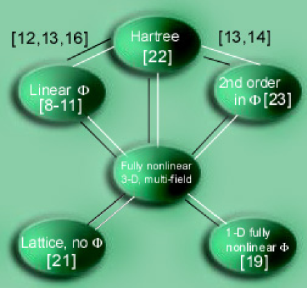
FIG. 1.: A schematic figure showing the numerical approaches to preheating with numbers in brackets denoting appropriate references. See the text for discussion.

Here we present first estimates of PBH production including backreaction computed dynamically. We find that while preheating may lead to over-production of PBH’s in some regions of parameter space, the result is sensitive to many subtle issues.

To place our methods in context, consider Fig. 1 which shows the different numerical studies of preheating undertaken in the literature. The eventual goal of these studies is a fully nonlinear analysis of multi-field preheating including metric perturbations. So far this has been achieved without metric perturbations (“no $\Phi$”) - often with simplified expansion dynamics - through lattice simulations [21]. The furthest the community has progressed [19] in solving the full Einstein field equations is in a model with plane wave symmetry and a single scalar field.

An alternative to full lattice simulations of preheating is the use of the Hartree, large-N, and mean field approximations [22]. Recently the Hartree approximation has been combined with the linear approximation for metric perturbations $\Phi$ [12, 17, 18] and, in [13, 14], with the second order metric perturbations formalism of Abramo et al. [23]. It is this latter approach that we adopt.

Immediate goals are fully nonlinear spherically symmetric simulations suitable for studying individual PBH formation (c.f. [24]) and inclusion of rescattering effects in the presence of metric perturbations, $\Phi$. The latter requires going beyond the Hartree approximation and evaluating double and triple convolutions.

The Model – We consider the two scalar field chaotic inflation model

$$V(\phi,\chi)=\frac{\lambda}{4}\phi^{4}+\frac{g^{2}}{2}\phi^{2}\chi^{2},$$ (1)

where $\phi$ is an inflaton field. During inflation $\chi$ decreases rapidly towards zero if $g^{2}/\lambda\gg 1$ in which case the temperature anisotropies in the CMB simply scale as $\Delta T/T\sim\sqrt{\lambda}$. We therefore choose a self-coupling of $\lambda=10^{-13}$. During preheating, $\chi$ and $\delta\chi_{k}$ grow exponentially in very specific geometric channels or resonance bands which are well understood in terms of Floquet theory[25, 10].

We assume a flat background FLRW geometry with perturbations in the longitudinal gauge[8]:

$$ds^{2}=-(1+2\Phi)dt^{2}+a^{2}(1-2\Phi)\delta_{ij}dx^{i}dx^{j},$$ (2)

where $\Phi=\Phi({\bf x},t)$, the natural generalization of the Newtonian potential, describes scalar perturbations and $a=a(t)$ is the scale factor. We decompose the scalar fields into homogeneous parts and fluctuations as $\phi(t,{\bf x})\to\phi(t)+\delta\phi(t,{\bf x})$ and $\chi(t,{\bf x})\to\chi(t)+\delta\chi(t,{\bf x})$.

The structure of the linearized Einstein field equations for this system can be schematically written in terms of two vectors: one for the FLRW background dynamics ${\bf X}=(\phi,\dot{\phi},\chi,\dot{\chi},a,\dot{a})$, and one for the perturbation variables in Fourier space: ${\bf Y}_{k}=(\delta\phi_{k},\delta\dot{\phi}_{k},\delta\chi_{k},\delta\dot{\chi}_{k},\Phi_{k},\zeta_{k})$.

While we solve the system of linearized Einstein field equations in the longitudinal gauge, it is convenient to calculate PBH constraints in terms of the curvature perturbation $\zeta_{k}$ rather than $\Phi_{k}$. $\zeta_{k}$ is defined in terms of $\Phi_{k}$ and the Hubble parameter, $H\equiv\dot{a}/a$, by

$$\zeta_{k}\equiv\Phi_{k}-\frac{H}{\dot{H}}\left(H\Phi_{k}+\dot{\Phi}_{k}\right),$$ (3)

and is usually conserved on super-Hubble scales in the adiabatic single field inflationary scenario. In the multi-field case which we consider in this paper, this quantity can change nonadiabatically due to the amplification of isocurvature (entropy) perturbations.

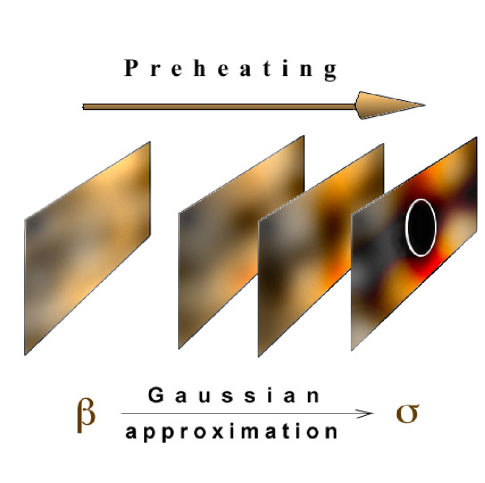
FIG. 2.: An illustration of primordial black hole (PBH) formation during preheating due to growth of density perturbations. The PBH event horizon is schematically shown by the white ring in the final panel. Astrophysical limits on PBH’s constrain $\beta$, the ratio of PBH to total energy density. To constrain theory one needs to map $\beta$ into the mass variance $\sigma$, most easily achieved with a Gaussian or chi-squared assumption for density perturbations. It is $\sigma$ that we calculate in our simulations.

We include backreaction effects to second order in both field and metric perturbations[23], which implies that we integrate coupled integro-differential equations. The precise structure of these equations and additional details can be found in Appendix and [12, 13, 14, 23]. Here we illustrate the skeletal structure of the system, which has the form

$$\dot{{\bf X}} = {\bf F}({\bf X},\langle{\bf Y}^{2}\rangle),$$ (4)

$$\dot{{\bf Y}}_{k} = {\bf G}({\bf X},\langle{\bf Y}^{2}\rangle)~{}{\bf Y}_{k},$$ (5)

$${\bf F} = {\bf F}_{\rm hom}+{\bf F}_{\rm pert},$$ (6)

$${\bf F}_{\rm pert} = {\bf F}_{\rm pert}(\langle\delta\phi^{2}\rangle,\langle\delta\chi^{2}\rangle,\langle\Phi^{2}\rangle,...)\,,$$ (7)

where the variance is defined by

$$\langle\diamond^{2}\rangle\equiv\frac{1}{2\pi^{2}}\int k^{2}|\diamond|_{k}^{2}dk\,,$$ (8)

for any field $\diamond$. ${\bf F}$ and ${\bf G}$ are nonlinear functions of the spatially homogeneous background vector ${\bf X}$ and the variances of the components of ${\bf Y}$. The complete system is integrated from 50 e-folds before the end of inflation to provide the appropriate initial conditions for preheating. The initial values at the start of inflation are chosen as $\phi=4m_{\rm pl}$ and $\chi=10^{-3}m_{\rm pl}$ with conformal vacuum states for the fluctuations. Including the field variances ensures total energy conservation at 1-loop.

Primordial black hole constraints – Since PBH’s form from large density fluctuations[26], it is an obvious concern that preheating might encounter problems with PBH constraints arising from the Hawking evaporation of small PBH’s or from overclosure of the universe ($\Omega_{\rm PBH}>1$) for heavy PBH’s.

To quantify this suspicion one needs to compute the mass function $\beta$[27, 29]:

$$\beta=\frac{\rho_{\rm PBH}}{\rho_{\rm TOT}}=\int_{\delta_{c}}^{\infty}P(\delta)~{}d\delta,$$ (9)

where $P(\delta)$ is the probability distribution of the density contrast, $\delta$, and $\delta_{c}$, $(\approx 0.7)$ [30], is the critical value at which PBH formation occurs in the radiation dominated era.

Usually one assumes a Gaussian distribution $P(\delta)=1/(\sqrt{2\pi}\sigma)\exp[-\delta^{2}/(2\sigma^{2})]$, where $\sigma$ is the mass variance at horizon crossing. Observational constraints imply that $\beta<10^{-20}$ over a very wide range of mass scales, which translates into a bound on the mass variance of $\sigma<\sigma_{*}=0.08$. $\sigma>\sigma_{*}$ corresponds to PBH over-production in the Gaussian distributed case. When the distribution is instead first order chi-squared – an approximation to the $\chi$ density fluctuations in preheating (see the later discussions) – the threshold is $\sigma_{*}=0.03$[20].

Defining the power-spectrum of the curvature perturbation as ${\cal P}_{\zeta}\equiv k^{3}|\zeta_{k}|^{2}/(2\pi^{2})$, the mass variance can be expressed as[20, 33]

$$\sigma^{2}=\left(\frac{4}{9}\right)^{2}\int_{0}^{\infty}\left(\frac{k}{aH}\right)^{4}{\cal P}_{\zeta}\tilde{W}(kR)\frac{dk}{k}.$$ (10)

We choose a Gaussian-filtered window function $\tilde{W}(kR)\equiv\exp(-k^{2}R^{2}/2)$ where $R\equiv 1/k_{*}$ is the artificial smoothing scale [33]. We can expect exponential increase of $\sigma$ due to the excitement of field and metric perturbations during preheating. We solved the Einstein equations (7) numerically, varying the ratio $g^{2}/\lambda$, and evaluated the mass variance with two cut-offs $k_{*}=aH$ and $k_{*}=10aH$ to investigate sensitivity to cut-off effects.

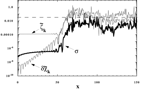
FIG. 3.: Threshold PBH formation – the growth of $\sigma$, $\tilde{\zeta}_{k}\equiv k^{3/2}\zeta_{k}$, and $\delta\tilde{\chi}_{k}\equiv k^{3/2}\delta\chi_{k}/m_{\rm pl}$ for a super-Hubble mode $\kappa\equiv k/(\sqrt{\lambda}\phi_{0})=10^{-22}$ vs dimensionless time $x\equiv\sqrt{\lambda}\phi_{0}\eta$ in the case $g^{2}/\lambda=2.5$, where $\phi_{0}\simeq 0.1m_{\rm pl}$ is the value of inflaton when it begins to oscillate coherently. With the choice $k_{*}=aH$ in the window function $\tilde{W}(kR)=\exp(-k^{2}R^{2}/2)$, $\sigma$ just reaches the threshold $\sigma_{*}=0.03$ for the PBH formation for chi-squared first order distributions.

When $\chi_{k}$ fluctuations are amplified during preheating, this stimulates the growth of the metric perturbation, $\Phi_{k}$. On cosmological scales this effect is sensitive to the suppression of $\chi$ and $\delta\chi_{k}$ modes in the preceding inflationary phase.

When $g^{2}/\lambda={\cal O}(1)$, this suppression is weak since the $\chi$ field is light [10] and once the long-wave $\delta\chi_{k}$ modes grow to of order $\delta\phi_{k}$ during preheating, super-Hubble $\Phi_{k}$ and $\zeta_{k}$ are amplified until backreaction effects shut off the resonance. This amplification occurs in the region $1<g^{2}/\lambda<3$[10, 11, 12, 13], where the $k\simeq 0$ modes lie in a resonance band. The increase in $\zeta_{k}$ leads to a corresponding growth of the mass variance $\sigma$ which can reach the threshold $\sigma_{*}=0.03$ for $1<g^{2}/\lambda<3$ and $6<g^{2}/\lambda<10$ with the cut-off set at $k_{*}=aH$, i.e., around the Hubble scale (see Fig. 3).

As $g^{2}/\lambda$ is increased, the $\chi$ field becomes heavy and suppressed during inflation. This restricts the amplification of super-Hubble metric perturbations [13] despite the fact that the $k\rightarrow 0$ mode of $\delta\chi_{k}$ lies in a resonance band for $n(2n-1)<g^{2}/\lambda<n(2n+1)$, $n=1,2,3...$ [25], as is evident from Fig. 4. However, since sub-Hubble $\delta\chi_{k}$ modes are not suppressed during inflation[14, 9], $\Phi_{k}$ and $\zeta_{k}$ on sub-Hubble scales do exhibit nonadiabatic, resonant, growth for $g^{2}/\lambda\gg 1$ , which leads to growth of $\sigma$.

However, we do not find that this is significant enough to lead to $\sigma>\sigma_{*}$ for $g^{2}/\lambda\gg 1$, except for very short intervals around $\dot{\phi}=0$, in contrast to the expectations of [20]. However, when we enlarge the cut-off frequency $k_{*}$ to $10aH$, we do find $\sigma>0.08$ in wide ranges of parameter space (see Fig. 5). Somewhat surprisingly, these super-threshold regions are all clustered around the super-Hubble resonance bands in $g^{2}/\lambda$ space.

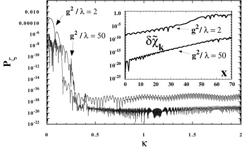
FIG. 4.: The power spectrum of $\zeta$ at the end of preheating for the values of $g^{2}/\lambda=2,50$ with $k_{*}=aH$. Since the inflationary suppression of $\chi$ becomes stronger as $g^{2}/\lambda$ is increased, the growth of $\zeta_{k}$ at long wavelengths is suppressed. Note also the dominance of the $g^{2}/\lambda=2$ modes at sub-Hubble scales $\kappa>1$. Inset : The evolution of $\delta\chi_{k}$ for a super-Hubble mode $\kappa\equiv k/(\sqrt{\lambda}\phi_{0})=10^{-22}$ for $g^{2}/\lambda=2,50$. The suppression of the initial conditions, due to the preceding inflationary phase, in the heavy case $g^{2}/\lambda=50$ is evident.

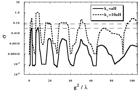
FIG. 5.: The mass variance $\sigma$ vs $g^{2}/\lambda$ for two window function cut-offs $k_{*}=aH$ and $k_{*}=10aH$. The threshold of $\sigma_{*}=0.03$ in the chi-squared distributed case is shown and is marginally crossed for the regions around $g^{2}/\lambda\sim 2$ and $g^{2}/\lambda\sim 8$ when $k_{*}=aH$. For $k_{*}=10aH$ a quilt of regions above the Gaussian threshold $\sigma_{*}=0.08$ emerges which coincide closely with $g^{2}/\lambda=2n^{2}$ corresponding to Floquet indices with maxima at longest wavelengths.

Initial conditions for the $\chi$ field – An issue of general importance which has been little studied is that of initial conditions for non-inflaton fields at the start of inflation. In our model these fields are represented by $\chi$ and the initial value is set $55$ e-folds before the end of inflation. This problem has two facets - the initial value of the background, or vacuum expectation value of $\chi$, and the initial value of the distribution of fluctuations, i.e., $\delta\chi_{k}$.

A sensible choice for the latter is the Bunch-Davis vacuum, but it is the initial value of the homogeneous part of $\chi$, which is of the most importance, since if $\chi=0$ (the minimum of the potential) no resonance can occur at linear order.

We have found four suggestions for setting the initial value, $\chi_{i}$, as follows.

(1) Choose the value of $\chi$ which maximises the probability distribution in eternal inflation for fixed large values of the inflaton ($\phi>1m_{\rm pl}$) at a specific time. Since the regions with the largest Hubble constant dominate the distribution [32] this corresponds to choosing $\chi>1m_{\rm pl}$, i.e., super-Planckian chaotic initial conditions for $\chi$.

This suggestion is, however, sensitive to the choice of a hypersurface for setting the initial conditions. If one defines initial conditions on the hypersurface of energy density equal to the Planck energy for instance, then the Hubble constant will likely be maximised by placing all energy into the field with the flatest potential, rather than distributing it amoung the various fields, some of which may have steep potentials. This will lead to vanishingly small initial $\chi$ unless $\chi$ is a good inflaton, i.e., $g^{2}~{}\mbox{\raisebox{-4.30554pt}{$\stackrel{{\scriptstyle\textstyle<}}{{\textstyle\sim}}$}}~{}\lambda$.

(2) Choose $\chi_{i}$ to satisfy $\chi_{i}^{2}=\langle\chi^{2}\rangle$ [13]. If we use the Bunch-Davis condition, $\chi_{k}\sim 1/\sqrt{\omega_{k}}\sim 1/\sqrt{g\phi}$, we can estimate $\langle\chi^{2}\rangle=\frac{1}{2\pi^{2}}\int k^{2}|\chi_{k}|^{2}dk$ to be $\sim k_{*}^{3}/(g\phi)$ if the variance is super-Hubble dominated during inflation and where $k_{*}=H$ is the natural cut-off at the Hubble scale.

Now if inflation is driven by $\phi$ then $H^{2}\simeq V(\phi)/m_{\rm pl}^{2}$ and we find $\chi_{i}^{2}\simeq V(\phi)^{3/2}/(g\phi m_{\rm pl}^{3})$. For the potential (1) this leads to the estimates $\chi_{i}\sim 10^{-5}m_{\rm pl}$ for $g^{2}/\lambda={\cal O}(1)$ and $\chi_{i}\sim 10^{-8}g^{-1/2}m_{\rm pl}$ for $g^{2}/\lambda\gg 1$ if we take $\lambda\sim 10^{-13}$ and $\phi_{i}\sim 4m_{\rm pl}$.

(3) Choose the value of $\chi_{i}$ which leads to a stationary distribution in eternal inflation (where the classical drift and quantum fluctuations are balanced) . Assuming quantum fluctuations $\delta\phi\sim H/2\pi$ on characteristic time scales $\delta t\sim H^{-1}$ one arrives at $\chi_{i}\sim H^{3}/(g^{2}\phi^{2})\sim\lambda^{3/2}\phi^{4}/(g^{2}m_{\rm pl}^{3})$ and hence $\chi_{i}\sim 10^{-4}-10^{-3}m_{\rm pl}$ for $g^{2}/\lambda={\cal O}(1)$ and $\chi_{i}\sim 10^{-16}g^{-2}m_{\rm pl}$ for $g^{2}/\lambda\gg 1$.

(4) Finally we may choose the value of $\chi_{i}$ which corresponds to the instantaneous minimum of the potential. It suggests $\chi_{i}=0$. This argument has several problems the most fundamental of which is that the system is not in equilibrium since the $\chi$ field is not strongly coupled except for $g^{2}/\lambda\gg 1$.

Despite the wide range of possible initial values, $\chi_{i}$, at the start of inflation, Fig. 6 shows that the final mass variance, and hence the probability of PBH over-production, depends rather weakly on $\chi_{i}$.

FIG. 6.: The smoothed dependence of the final mass variance $\sigma$ on the initial condition, $\chi_{i}$, 55 e-folds before the start of preheating for $g^{2}/\lambda=2,50$. Note the relatively weak dependence in both cases.

Potential problems and unresolved issues – Our results suggest that PBH over-production may not be generic in strong preheating. However they can only be considered as preliminary for a number of reasons:

• There are at least two fields critically involved in preheating. Even if the inflationary fluctuations are Gaussian, the fluctuations induced by preheating are typically not. If the $\chi$ field has no vacuum expectation value, its density fluctuations are roughly $\propto\delta\chi^{2}$, so approximately chi-squared if $\delta\chi$ is Gaussian distributed. As discussed above, we take $\chi\neq 0$. The recent results of [31] suggest that $\chi$ is Gaussian distributed before rescattering sets in and hence the density perturbations would be Gaussian, at least while dominated by linear fluctuations.

  Rescattering leads to non-Gaussian distributions and to $\delta\phi\propto\delta\chi^{2}$ [7]. The applicability of the criterion $\sigma>\sigma_{*}$ therefore depends largely on when PBH formation actually takes place - before or after rescattering.

  Further, the density fluctuations may go nonlinear. Since $\delta\in[-1,\infty)$ this necessarily skews the distribution, similar to the toy-model discussed in the second Ref. of [27]. Non-Gaussianity may drastically alter the relationship between $\beta$ and $\sigma$ [27, 28], changing $\sigma_{*}$ and requiring the use of higher-order statistics.

• In preheating the Hubble radius is vastly smaller than the true particle horizon and resonance bands often cover the complete range of scales. Predicting the mass spectrum of PBH’s created during preheating is therefore a subtle issue. Crudely one expects a wide range of PBH masses to be produced, even without criticality arguments [30].

  This is related to our results showing cut-off, $k_{*}$, sensitivity. The increase in $\sigma$ when $k_{*}$ is altered from $aH$ to $10aH$ reflects the important contributions of sub-Hubble modes. Does this necessarily imply that the resulting PBH’s are very small ? If so, they are not constrained since they evaporate harmlessly long before nucleosynthesis.

• We have not included rescattering. This is known to enhance variances over the Hartree approximation at small resonance parameters, $q$, in the absence of metric perturbations[21]. For $q\gg 1$ however, the situation is reversed and variances are overestimated by the Hartree approximation. Whether these results are stable to inclusion of metric perturbations is unknown, but this may provide a way to avoid PBH over-production since it should filter through to $\zeta_{k}$ and $\sigma$.

• Fig. 5 shows $\sigma$ as a function of $g^{2}/\lambda$. The value of $\sigma$ plotted is its maximum at the end of preheating. However, $\sigma$ does grow larger than this value, instantaneously exceeding $0.01$, even for $k_{*}=aH$, when $\dot{\phi}=0$. We choose the more conservative route of not taking these as the true maxima, but the question remains, can large $\sigma$, attained for very short periods, lead to PBH formation ?

• We solved the $\chi$ field equation, including second order terms such as $\langle\Phi\delta\ddot{\chi}\rangle$[14]. Initially $\delta\chi$ and $\Phi$ are correlated but when the $\chi$ fluctuations are sufficiently amplified, they are well described by classical stochastic waves[17], which may be uncorrelated with metric variables.

  It is uncertain that contributions of second order metric terms should be included during such classical regimes. Since this issue affects $\chi$ rather significantly, the quantum to classical transition appears to be of quantitative importance, deserving further study.

Conclusions – We have studied primordial black hole (PBH) formation during preheating using numerical simulations of the perturbed Einstein field equations including second order field and metric backreaction effects. We found that there exist parameter ranges where standard Gaussian and chi-squared thresholds for PBH formation are exceeded.

Nevertheless, the results are not unambiguous. We discovered a significant sensitivity to the window function cut-off, $k_{*}$, and since preheating is expected to lead to non-Gaussian fluctuations, it is not clear how realistic the Gaussian threshold for PBH formation is. Nevertheless, PBH over-production constraints are very robust. The study of PBH’s in preheating is an exciting area which may lead to strong constraints on realistic inflationary models.

We note that there are a number of possible escape routes to preserve preheating but avoid PBH over-production. Fermionic preheating is very unlikely to lead to PBH formation unless the fermions are extremely massive. Similarly, instant preheating [34], which draws energy away from the $\chi$ field almost immediately seems likely to stall PBH formation, as does a large $\chi$ self-interaction.

On the other hand, since growth of $\zeta_{k}$ and $\sigma$ is seeded through isocurvature/entropy perturbations [16], it is possible that other models of reheating, such as non-oscillatory models [35], which lead to significant isocurvature modes, may also have a PBH over-production problem.

Nevertheless, the precise scenario of the PBH formation during preheating can only be understood properly by overcoming two serious hurdles - (1) understanding the probability distribution of density fluctuations during preheating and (ii) going to fully nonlinear simulations of resonant PBH formation which include rescattering and nonlinear metric perturbations.

Acknowledgements – We thank Christopher Gordon, Alan Guth, Anne Green, Roy Maartens, Kei-ichi Maeda, Karim Malik, Masaaki Morita, and Takashi Torii for useful discussions and comments.

Appendix: Detailed form of the evolution equations

In this Appendix we present the evolution equations in details. We include second order field and metric backreaction effects[23] in the background equations, which is combined with the Hartree approximation[22].

Then the Hubble parameter and homogeneous parts of the scalar fields satisfy[13, 14]:

$$H^{2} = \frac{8\pi G}{3}\Biggl{[}\frac{1}{2}\dot{\phi}^{2}+\frac{1}{2}\langle\delta\dot{\phi}^{2}\rangle+\frac{1}{2a^{2}}\langle(\nabla\delta\phi)^{2}\rangle$$ (11)

$$+ \frac{1}{2}\dot{\chi}^{2}+\frac{1}{2}\langle\delta\dot{\chi}^{2}\rangle+\frac{1}{2a^{2}}\langle(\nabla\delta\chi)^{2}\rangle$$ (12)

$$+ \frac{1}{4}\lambda(\phi^{4}+6\phi^{2}\langle\delta\phi^{2}\rangle+3\langle\delta\phi^{2}\rangle^{2})+\frac{1}{2}g^{2}\phi^{2}\langle\chi^{2}\rangle$$ (13)

$$+ 2(\lambda\phi^{3}+g^{2}\phi\chi^{2})\langle\Phi\delta\phi\rangle+2g^{2}\phi^{2}\chi\langle\Phi\delta\chi\rangle\Biggr{]}$$ (14)

$$+ 4H\langle\Phi\dot{\Phi}\rangle-\langle\dot{\Phi}^{2}\rangle+\frac{3}{a^{2}}\langle(\nabla\Phi)^{2}\rangle,$$ (15)

$$(\ddot{\phi} + 3H\dot{\phi})(1+4\langle\Phi^{2}\rangle)+\lambda\phi(\phi^{2}+3\langle\delta\phi^{2}\rangle)$$ (16)

$$+ g^{2}(\chi^{2}+\langle\delta\chi^{2}\rangle)\phi-2\langle\Phi\delta\ddot{\phi}\rangle-4\langle\dot{\Phi}\delta\dot{\phi}\rangle$$ (17)

$$- 6H\langle\Phi\delta\dot{\phi}\rangle+4\dot{\phi}\langle\dot{\Phi}\Phi\rangle-\frac{2}{a^{2}}\langle\Phi\nabla^{2}(\delta\phi)\rangle=0,$$ (18)

$$(\ddot{\chi} + 3H\dot{\chi})(1+4\langle\Phi^{2}\rangle)+g^{2}(\phi^{2}+3\langle\delta\phi^{2}\rangle)\chi$$ (19)

$$- 2\langle\Phi\delta\ddot{\chi}\rangle-4\langle\dot{\Phi}\delta\dot{\chi}\rangle-6H\langle\Phi\delta\dot{\chi}\rangle$$ (20)

$$+ 4\dot{\chi}\langle\dot{\Phi}\Phi\rangle-\frac{2}{a^{2}}\langle\Phi\nabla^{2}(\delta\chi)\rangle=0,$$ (21)

where $G\equiv m_{\rm pl}^{-2}$ is Newton’s gravitational constant. Note that $\langle...\rangle$ implies a spatial average. In spite of the exponential suppression during inflation, operative when the $\chi$ field is heavy ($g^{2}/\lambda\gg 1$), the $\chi$ field can be significantly enhanced in the presence of the second order metric backreaction terms in Eq. (21) as pointed out in Ref. [14].

The Fourier transformed, perturbed Einstein equations are

$$\delta\ddot{\phi}_{k} + 3H\delta\dot{\phi}_{k}$$ (22)

$$+ \left[\frac{k^{2}}{a^{2}}+3\lambda(\phi^{2}+\langle\delta\phi^{2}\rangle)+g^{2}(\chi^{2}+\langle\delta\chi^{2}\rangle)\right]\delta\phi_{k}$$ (23)

$$= 4\dot{\phi}\dot{\Phi}_{k}+2(\ddot{\phi}+3H\dot{\phi})\Phi_{k}-2g^{2}\phi\chi\delta\chi_{k},$$ (24)

$$\delta\ddot{\chi}_{k} + 3H\delta\dot{\chi}_{k}+\left[\frac{k^{2}}{a^{2}}+g^{2}(\phi^{2}+\langle\delta\phi^{2}\rangle)\right]\delta\chi_{k}$$ (25)

$$= 4\dot{\chi}\dot{\Phi}_{k}+2(\ddot{\chi}+3H\dot{\chi})\Phi_{k}-2g^{2}\phi\chi\delta\phi_{k},$$ (26)

$$\dot{\Phi}_{k}+H\Phi_{k}=4\pi G(\dot{\phi}\delta\phi_{k}+\dot{\chi}\delta\chi_{k}).$$ (27)

We find from Eq. (27) that metric perturbations grow if $\chi$ and $\delta\chi_{k}$ fluctuations are amplified during preheating and the $\chi$-dependent source term exceeds the $\phi$-dependent one. When field and metric fluctuations are sufficently amplified, the coherent oscillations of the inflaton condensate, $\phi$, are destroyed. The entire spectrum of fluctuations typically moves out of the dominant resonance band and the resonance is shut off.

REFERENCES

- [1] S. W. Hawking and N. Turok, Phys. Lett. B 425, 25 (1998); S. W. Hawking and H. S. Reall, Phys. Rev. D 59, 023502 (1999); A. Vilenkin, ibid. 58, 067301 (1998); V. Vanchurin, A. Vilenkin, and S. Winitzki, ibid. 61 083507 (2000).
- [2] D. Goldwirth and T. Piran, Phys. Rev. Lett. 64, 2852 (1990); T. Vachaspati and M. Trodden, Phys. Rev. D 61 023502 (2000).
- [3] D. H. Lyth and A. Riotto, Phys. Rep. 314, 1 (1999).
- [4] A. H. Guth and E. J. Weinberg, Nucl. Phys. B212, 321 (1983).
- [5] M. Gasperini, J. Maharana, and G. Veneziano, Nucl. Phys. B 472, 349 (1996).
- [6] G. F. Giudice, A. Riotto, and I. I. Tkachev, JHEP 9911, 036 (1999); D. H. Lyth, Phys. Lett. B 469, 69 (1999); R. Kallosh, L. Kofman, A. Linde, and A. Van Proeyen, Phys. Rev. D 61, 103503 (2000).
- [7] L. Kofman, A. Linde, and A. A. Starobinsky, Phys. Rev. D 56, 3258 (1997).
- [8] B. A. Bassett, D. I. Kaiser, and R. Maartens, Phys. Lett. B 455, 84 (1999); B. A. Bassett, F. Tamburini, D. I. Kaiser, and R. Maartens, Nucl. Phys. B 561, 188 (1999).
- [9] B. A. Bassett, C. Gordon, R. Maartens, and D. I. Kaiser, Phys. Rev. D 61, 061302 (R) (2000).
- [10] B. A. Bassett and F. Viniegra, Phys. Rev. D 62, 043507 (2000).
- [11] F. Finelli and R. Brandenberger, Phys. Rev. D 62, 083502 (2000).
- [12] S. Tsujikawa, B. A. Bassett, and F. Viniegra, JHEP 08, 019 (2000); S. Tsujikawa and B. A. Bassett, Phys. Rev. D 62, 045310 (2000).
- [13] Z. P. Zibin, R. H. Brandenberger, and D. Scott, hep-ph/0007219 (2000).
- [14] K. Jedamzik and G. Sigl, Phys. Rev. D 61, 023519 (2000).
- [15] P. Ivanov, Phys. Rev. D 61, 023505 (2000).
- [16] A. R. Liddle et al., Phys. Rev. D 61, 103509 (2000).
- [17] A. B. Henriques and R. G. Moorhouse, Phys. Rev. D 62, 063512 (2000).
- [18] S. Tsujikawa, JHEP 07, 024 (2000).
- [19] M. Parry and R. Easther, Phys. Rev. D 62, 103503 (2000).
- [20] A. M. Green and K. A. Malik, hep-ph/0008113 (2000).
- [21] S. Yu. Khlebnikov and I. I. Tkachev, Phys. Rev. Lett. 79, 1607 (1997); T. Prokopec and T. G. Roos, Phys. Rev. D 55, 3768 (1997); S. Kasuya and M. Kawasaki, ibid. 58, 083516 (1998); M. Parry and A. T. Sornborger, ibid. 60, 103504 (1999); A. Rajantie and E. J. Copeland, Phys. Rev. Lett. 85, 916 (2000).
- [22] S. Yu. Khlebnikov, I. I. Tkachev, Phys. Lett. B 390 80 (1997); S. A. Ramsey and B. L. Hu, Phys. Rev. D 56, 678 (1997); D. Boyanovsky et al., ibid. 56, 1939 (1997); S. Tsujikawa, K. Maeda, and T. Torii, ibid. 60, 063515 (1999); 123505 (1999); J. Baacke and C. Patzold, ibid. 61, 024016 (2000); B. A. Bassett and F. Tamburini, Phys. Rev. Lett. 81, 2630 (1998).
- [23] L. R. Abramo, R. H. Brandenberger, and V. M. Mukhanov, Phys. Rev. D 56, 3248 (1997).
- [24] J. Balakrishna, E. Seidel, and W.-M. Suen, Phys. Rev. D 58, 104004 (1998).
- [25] P. B. Greene, L. Kofman, A. Linde, and A. A. Starobinsky, Phys. Rev. D 56, 6175 (1997).
- [26] B. J. Carr and S. W. Hawking, Mon. Not. Roy. Astron. Soc. 168, 399 (1974); B. J. Carr, Astrophys. J. 205, 1 (1975).
- [27] J. S. Bullock and J. Primack, Phys. Rev. D 55, 7423 (1997); ibid. astro-ph/9806301.
- [28] P. Ivanov, Phys. Rev. D 57, 7145 (1998).
- [29] A. M. Green and A. R. Liddle, Phys. Rev. D 56, 6166 (1997); A. M. Green, A. R. Liddle, and A. Riotto, ibid. 7554 (1997).
- [30] J. C. Niemeyer and K. Jedamzik, Phys. Rev. Lett. 80, 5481 (1998); ibid. Phys. Rev. D 59, 124013 (1999).
- [31] G. Felder and L. Kofman, hep-ph/0011160.
- [32] S. Winitzki and A. Vilenkin, Phys. Rev. D 61 084008 (2000).
- [33] A. R. Liddle and D. H. Lyth, Phys. Rep. 231, 1 (1993).
- [34] G. Felder, L. Kofman, A. Linde, Phys. Rev. D59, 123523 (1999).
- [35] G. Felder, L. Kofman, A. Linde, Phys. Rev. D60, 103505 (1999).