Domain walls in QCD

Abstract:

QCD was shown to have a nontrivial vacuum structure due to the topology of the $\theta\equiv\theta+2\pi n$ parameter. As a result of this nontrivial topology, in the large $N_{c}$ limit, quasi-stable QCD domain walls appear, characterized by a transition in the singlet $\eta^{\prime}$ field. We discuss the physics of these QCD domain walls as well as related axion domain walls and we present a new type of axion wall which also contains an $\eta^{\prime}$ transition. We argue that these domain walls are topologically stable in the limit $N_{c}\rightarrow\infty$ and classically stable for large but finite $N_{c}$, however, they can decay through a tunneling process. We argue that the qualitative features of these QCD domain walls — namely their classical stability — persist to the realistic case of $N_{c}=3$ and that it is at least possible that their lifetime could be macroscopically large. If it is, then QCD domain walls could play an important role in the evolution of early universe and may be detectable in energetic collisions such as those at the Relativistic Heavy Ion Collider (RHIC).

1 Introduction

Colour confinement, spontaneous breaking of chiral symmetry, the $\mathop{\rm{}U}(1)$ problem, $\theta$ dependence, and the classification of vacuum states are some of the most interesting topics in QCD. Unfortunately, the progress in our understanding of them is extremely slow. At the end of the 1970s A. M. Polyakov [1] demonstrated colour confinement in $3$-dimensional QED (QED₃): this was the first example in which nontrivial dynamics of the ground state played a key role. Many papers were written regarding the ground state structure of gauge theories in the strong coupling regime, but there were many unanswered questions. Almost 20 years passed before the next important piece of the puzzle was solved [2, 3]. Seiberg and Witten demonstrated that confinement occurs in supersymmetric (SUSY) QCD₄ due to the condensation of monopoles: a similar mechanism was suggested many years ago by ’t Hooft and Mandelstam (see [4] for a review). Furthermore, condensation of dyons together with oblique confinement for nonzero vacuum angle $\theta$ was also discovered in SUSY models [5] (this phenomenon was also argued to take place in ordinary QCD. See [4]).

In addition to providing solid demonstration of earlier ideas, the recent progress in SUSY models has introduced many new phenomena, such as the existence of rich vacuum state structure and the existence of domain walls [6]: topologically stable interpolations connecting the same vacuum state. The same conclusion was reached by Witten in [7, 8] based on a D-brane construction in the limit of large $N_{c}$. In fact, one can see that in both approaches, the number of states in the vacuum family is $N_{c}$. Motivated by this development in SUSY gauge theories D-brane construction, we ask how this applies to QCD. The issue of classifying the vacuum states for a given parameter $\theta$ as well as the phenomenological consequences (domain walls and their decay etc. ) is the subject of this work. In separate publications [9] we shall apply these results to analyze the physics after the QCD phase transition in evolution of early Universe. In particular, we discuss the possibility of generation of primordial magnetic fields due to the existence of short-lived QCD domain walls discussed in this paper.

The starting point of our analysis is an effective Lagrangian approach. Experience with SUSY models demonstrates that the effective Lagrangian approach is a very effective tool for the analysis of large distance dynamics in the strong coupling regime. There are two different definitions of an effective Lagrangian in quantum field theory. One of them is the Wilsonian effective Lagrangian describing the low energy dynamics of the lightest particles in the theory. In QCD, this is implemented by effective chiral Lagrangians for the pseudoscalar mesons. Another type of effective Lagrangian is defined by taking the Legendre transform of the generating functional for connected Green’s functions to obtain an effective potential. This object is useful in addressing questions about the vacuum structure of the theory in terms of vacuum expectation values (VEVs) of composite operators — these VEVs minimize the effective action. The latter approach is well suited for studying the dependence of the vacuum state on external parameters such as the light quark masses or the vacuum angle $\theta$. However, it is not, for example, useful for studying $S$-matrix elements because the kinetic term cannot be recovered through this approach. The utility of the second approach for gauge theories had been recognized long ago for supersymmetric models, where the anomalous effective potential was found for both the pure supersymmetric gluodynamics [10] and supersymmetric QCD (SQCD) [11] models. Properties of the vacuum structure in the SUSY models were correctly understood only after analyzing this kind of effective potential.

This paper contains many of the details mentioned in the letter [9] and is organized as follows:

Section 2:

Here we review the properties of the QCD effective Lagrangian [12, 13] which is a generalization of the Di Vecchia-Veneziano-Witten (VVW) Lagrangian [14, 15] to include terms subleading in $1/N_{c}$ as well as to account for a constraint due to the quantization topological charge. One should emphasize from the very beginning that the specific form of the effective potential used in this paper is not critical for the present analysis: only the topological structure and winding $\theta\rightarrow\theta+2\pi n$ — a consequence of the topological charge quantization — is essential.

Section 3:

Here we review the idea of topological charge conservation and argue that, in the limit $N_{c}\rightarrow\infty$, the QCD effective Lagrangian admits stable domain walls. We then discuss how these walls are metastable on the quantum level due to a tunnelling decay mode allowed when we consider heavier degrees of freedom to the next order in $1/N_{c}$.

Section 4:

Here we present the classical domain wall solutions for QCD domain walls both with and without a dynamical axion field.

Section 5:

Here we show that the QCD domain walls are not stable on the quantum level due to a tunnelling phenomena as discussed in Section 3. In this section we also discuss the validity of the large $N_{c}$ approximation when $N_{c}=3$ and argue that the realistic case is qualitatively the same as the large $N_{c}$ limit. We estimate the lifetime of the QCD domain walls when $N_{c}=3$ and show that it is potentially macroscopically large. Thus, these domain walls may play an important role in various physical processes.

Section 6:

This is our conclusion.

2 Effective Lagrangian and $\theta$ dependence in QCD

Our analysis begins with the effective low energy QCD action derived in [12, 13], which allows the $\theta$-dependence of the ground state to be analyzed. Within this approach, the pseudo-Goldstone fields and $\eta^{\prime}$ field are described by the unitary matrix $U_{ij}$, which correspond to the $\gamma_{5}$ phases of the chiral condensate: $\langle\overline{\Psi}_{L}^{i}\Psi_{R}^{j}\rangle=-|\langle\overline{\Psi}_{L}\Psi_{R}\rangle|\,U_{ij}$ with

$$U=\exp\left[i\sqrt{2}\,\frac{\pi^{a}\lambda^{a}}{f_{\pi}}+i\frac{2}{\sqrt{N_{f}}}\frac{\eta^{\prime}}{f_{\eta^{\prime}}}\right],\quad UU^{\dagger}=1\,,$$ (1)

where $\lambda^{a}$ are the Gell-Mann matrices of $\mathop{\rm SU}(N_{f})$, $\pi^{a}$ is the pseudoscalar octet, and $f_{\pi}=133$ MeV. In terms of $U$ the low-energy effective potential is given by [12, 13]:

$$W_{{\rm QCD}}(\theta,U)=\\ -\lim_{V\rightarrow\infty}\frac{1}{V}\,\log\sum_{l=0}^{N_{c}-1}\exp\Biggl{\{}\frac{V}{2}{\rm Tr}(MU+\text{H.c.})\,+VE\cos\left(\frac{2\pi l+i\log{\rm Det}~{}U-\theta}{N_{c}}\right)\Biggr{\}}.$$ (2)

All dimensional parameters in this potential are expressed in terms of the QCD vacuum condensates, and are well known: $M={\rm diag}(m_{q}^{i}|\langle\bar{\Psi}^{i}\Psi^{i}\rangle|)$; the constant $E$ is related to the QCD gluon condensate $E=\langle\frac{b\alpha_{s}}{32\pi}G^{2}\rangle$, where numerically $3b=11N_{c}-2N_{f}$; the quark condensate $\langle\bar{\Psi}^{i}\Psi^{i}\rangle\simeq-(240\;{\rm MeV})^{3}$, and the gluon condensate $\langle\frac{\alpha_{s}}{\pi}G^{2}\rangle\simeq 1.2\times 10^{-2}{\rm GeV}^{4}$.

It is possible to argue that Equation (2) represents the anomalous effective Lagrangian realizing broken conformal and chiral symmetries of QCD. The arguments are that Equation (2):

1. correctly reproduces the VVW effective chiral Lagrangian, [14, 15] in the large $N_{c}$ limit,

   [For small values of $(\theta-i\log{\rm Det}\,U)$, the term with $l=0$ dominates the infinite volume limit. Expanding the cosine (this corresponds to the expansion in $1/N_{c}$), we recover exactly the VVW effective potential [14, 15] together with the constant term $-E=-\langle b\alpha_{s}/(32\pi)G_{\mu\nu}^{2}\rangle$ required by the conformal anomaly:

   $$W_{VVW}(\theta,U,U^{\dagger})=-E-\frac{1}{2}{\rm Tr}(MU+\text{H.c.})+\frac{1}{2}\langle\nu^{2}\rangle_{YM}(i\log{\rm Det}\,U-\theta)^{2}\ldots\;,$$ (3)

   where we used the fact that at large $N_{c}$, $E/N_{c}^{2}=-\langle\nu^{2}\rangle_{YM}$ is the topological susceptibility in pure YM theory. Corrections in $1/N_{c}$ stemming from Equation (2) constitute a new result of [12, 13].]

2. reproduces the anomalous conformal and chiral Ward identities of QCD,

   [Let us check that the anomalous Ward Identities (WI’s) in QCD are reproduced from Equation (2). The anomalous chiral WI’s are automatically satisfied with the substitution $\theta\rightarrow(\theta-i\log{\rm Det}\,U)$ for any $N_{c}$, in accord with  [14, 15]. Furthermore, it can be seen that the anomalous conformal WI’s of [17] for zero momentum correlation functions of the operator $G_{\mu\nu}^{2}$ in the chiral limit $m_{q}\rightarrow 0$ are also satisfied when $E$ is chosen as above. As another important example of WI’s, the topological susceptibility in QCD near the chiral limit will be calculated from Equation (2). For simplicity, the limit of $\mathop{\rm SU}(N_{f})$ isospin symmetry with $N_{f}$ light quarks, $m_{q}\ll\Lambda_{{\rm QCD}}$ will be considered. For the vacuum energy for small $\theta$ one obtains  [12, 13]

   $$E_{{\rm vac}}(\theta)=-E+m_{q}\langle\bar{\Psi}\Psi\rangle N_{f}\cos\left(\frac{\theta}{N_{f}}\right)+{\rm O}(m_{q}^{2})\,.$$ (4)

   Differentiating this expression twice with respect to $\theta$ reproduces the chiral Ward identities [18, 19]:

   $$\lim_{q\rightarrow 0}\;i\int dx\,e^{iqx}\langle 0|T\left\{\tfrac{\alpha_{s}}{8\pi}G\tilde{G}(x)\,\tfrac{\alpha_{s}}{8\pi}G\tilde{G}(0)\right\}|0\rangle =-\frac{\partial^{2}E_{{\rm vac}}(\theta)}{\partial\,\theta^{2}}$$ (5)

   $$=\frac{1}{N_{f}}m_{q}\langle\bar{\Psi}\Psi\rangle+{\rm O}(m_{q}^{2})\;.$$

   Other known anomalous WI’s of QCD can be reproduced from Equation (2) in a similar fashion. Consequently, Equation (2) reproduces the anomalous conformal and chiral Ward identities of QCD, and in this sense passes the test for it to be the effective anomalous potential for QCD.]

3. reproduces the known $\theta$ dependence [14, 15].
     [As mentioned earlier, our results are similar to those found in  [14, 15]. A new element which was not discussed in 80’s, is the procedure of summation over $l$ in (2). As we shall discuss in a moment, this leads to the cusp structure of the effective potential which seems to be an unavoidable consequence of the topological charge quantization. These singularities are analogous to the ones arising in SUSY models and show the non-analyticity of phases at certain values of $\theta$. The origin of this non-analyticity is clear, it appears when the topological charge quantization is imposed explicitly at the effective Lagrangian level.]

In general, the $\theta$ dependence appears in the combination $\theta/N_{c}$, (see Equation (2)) which naïvely does not provide the desired $2\pi$ periodicity in the physical observables. Equation (2), however, explicitly demonstrates the $2\pi$ periodicity of the partition function. This seeming contradiction is resolved by noting that in the thermodynamic limit, $V\rightarrow\infty$, only the term of lowest energy in the summation over $l$ is retained for a particular value of $\theta$. The result is that the local geometry of any particular $\theta$ state, gives the illusion of $\theta/N_{c}$ periodicity in the observables, but when one considers the full topology of all the $\theta$ states and properly switches to the lowest energy branch, one regains the true $\theta$ periodicity. Of course, the values $\theta$ and $\theta+2\pi n$ are physically equivalent for the entire set of states, but relative transitions — switching branches — between different $\theta$ states have physical significance. It is exactly these transitions — resulting from the non-local effects of the topology of the fields — that are responsible for the domain walls we discuss in this paper.

When considering only the lightest degrees of freedom, as we do in the thermodynamic limit $V\rightarrow\infty$ of (2), the effective potential acquires a cusp singularity where one switches from one branch of the potential to another. These cusps represent physical transitions in heavier degrees of freedom which have been integrated out to get the low-energy effective potential (2). The physical effects of these heavier degrees of freedom will be discussed in Sections 5.2 and 5.4. The reader is referred to the original papers [12, 13] for more detailed discussions of the properties of the effective potential (2).

Our final remark regarding (2). The appearance of the cosine interaction, $\cos(\theta/N_{c})$, implies the following scenario in pure gluodynamics ($\phi_{i}$’s frozen): the $(2k)^{\rm th}$ derivative of the vacuum energy with respect to $\theta$, as $\theta\rightarrow 0$, is expressed solely in terms of one parameter, $1/N_{c}$, for arbitrary $k$:

$$\left.\frac{\partial^{2k}E_{{\rm vac}}(\theta)}{\partial\,\theta^{2k}}\right|_{\theta=0}\sim\int\prod_{i=1}^{2k}d^{4}x_{i}\left\langle Q(x_{1})...Q(x_{2k})\right\rangle\sim\left(\frac{i}{N_{c}}\right)^{2k},$$ (6)

where, $Q=\frac{\alpha_{s}}{8\pi}G\tilde{G}$. This property was seen as a consequence of Veneziano’s solution of the $\mathop{\rm{}U}(1)$ problem [20]. The reason that only one factor appears in Veneziano’s calculation is that the corresponding correlation function, $\sim\int\prod_{i=1}^{2k}d^{4}x_{i}\langle Q(x_{1})\cdots$ $Q(x_{2k})\rangle$, becomes saturated at large distances by the Veneziano ghosts whose contributions factorize exactly, and was subsequently interpreted as a manifestation of the $\theta/N_{c}$ dependence in gluodynamics at small $\theta$. However, at that time it was incorrectly assumed that such a dependence indicates that the periodicity in $\theta$ is proportional to $2\pi N_{c}$. We now know that the standard $2\pi$ periodicity in gluodynamics is restored by the summation over $l$ in (2) such that one jumps from one branch to another at $\theta=\pi$.

2.1 Vacuum states

In the next section we shall discuss different types of domain walls which interpolate between various vacuum states, but first we should study the classification of vacuum states themselves. In order to do so, it is convenient to parameterize the fields $U$ as

$$U=\left(\begin{array}[]{cccc}e^{i\phi_{1}}&0&\cdots&0\\ 0&e^{i\phi_{2}}&\cdots&0\\ \vdots&\vdots&\ddots&0\\ 0&0&0&e^{i\phi_{N_{f}}}\end{array}\right)$$ (7)

such that the potential (2) takes the form

$$V(\phi_{i},\theta)=-E\cos\left(\frac{1}{N_{c}}\theta-\frac{1}{N_{c}}\sum\phi_{i}\right)-\sum M_{i}\cos\phi_{i}\,.$$ (8)

The minimum of this potential is determined by the following equation:

$$\frac{1}{N_{c}}\sin\left(\frac{1}{N_{c}}\theta-\frac{1}{N_{c}}\sum\phi_{i}\right)=\frac{M_{i}}{E}\,\sin\phi_{i}\,,\qquad i=1,\ldots,N_{f}\,.$$ (9)

At lowest order in $1/N_{c}$ this equation coincides with that of [14, 15]. For general values of $M_{i}/E$, it is not possible to solve Equation (9) analytically, however, in the realistic case $\varepsilon_{u},\varepsilon_{d}\ll 1\,,\,\varepsilon_{s}\sim 1$ where $\varepsilon_{i}=N_{c}M_{i}/E$, the approximate solution can be found:

$$\sin\phi_{u} = \frac{m_{d}\sin\theta}{[m_{u}^{2}+m_{d}^{2}+2m_{u}m_{d}\cos\theta]^{1/2}}+{\rm O}(\varepsilon_{u},\varepsilon_{d})\,,$$

$$\sin\phi_{d} = \frac{m_{u}\sin\theta}{[m_{u}^{2}+m_{d}^{2}+2m_{u}m_{d}\cos\theta]^{1/2}}+{\rm O}(\varepsilon_{u},\varepsilon_{d})\,,$$

$$\sin\phi_{s} = {\rm O}(\varepsilon_{u},\varepsilon_{d})\,.$$ (10)

This solution coincides with the one of [14, 15] to leading order in $\varepsilon_{u},\varepsilon_{d}$. In what follows for the numerical estimates and for simplicity we shall use the $\mathop{\rm SU}(2)$ limit $m_{u}=m_{d}\ll m_{s}$ where the solution (10) can be approximated as:

$$\phi_{u} \simeq\theta/2, \phi_{d} \simeq\theta/2, \phi_{s} \simeq 0, 0\leq \;\theta<\pi,$$ (11)

$$\phi_{u} \simeq(\theta+2\pi)/2, \phi_{d} \simeq(\theta-2\pi)/2, \phi_{s} \simeq 0, \pi\leq \;\theta<2\pi, \text{etc}.$$

Once solution (11) is known, one can calculate the vacuum energy and topological charge density $Q=\langle 0|\tfrac{\alpha_{s}}{8\pi}G\tilde{G}|0\rangle$ as a function of $\theta$. In the limit $m_{u}=m_{d}\equiv m$, $\langle\bar{d}d\rangle=\langle\bar{u}u\rangle\equiv\langle\bar{\Psi}\Psi\rangle$ one has:

$$V_{{\rm vac}}(\theta) \simeq V_{\theta=0}+2m\big{|}\!\langle\bar{\Psi}\Psi\rangle\!\big{|}\left(1-\bigl{|}\cos\frac{\theta}{2}\bigr{|}\right)$$

$$\langle\theta|\tfrac{\alpha_{s}}{8\pi}G\tilde{G}|\theta\rangle = -\frac{\partial V_{{\rm vac}}(\theta)}{\partial\theta}=-m\big{|}\!\langle 0|\bar{\Psi}\Psi|0\rangle\!\big{|}\sin\frac{\theta}{2}\,.$$ (12)

As expected, the $\theta$ dependence appears only in combination with $m$ and goes away in the chiral limit. One can also calculate the chiral condensate $\langle\bar{\Psi}^{i}_{L}\Psi^{i}_{R}\rangle$ in the $\theta$ vacua using solution (11) for vacuum phases:

$$\langle\theta|\bar{\Psi}\Psi|\theta\rangle = \cos\frac{\theta}{2}\;\langle 0|\bar{\Psi}\Psi|0\rangle_{\theta=0}\,,$$

$$\langle\theta|\bar{\Psi}i\gamma_{5}\Psi|\theta\rangle = -\sin\frac{\theta}{2}\;\langle 0|\bar{\Psi}\Psi|0\rangle_{\theta=0}\,.$$ (13)

A remark is in order. As is well known, in thermal equilibrium and in the limit of infinite volume, the $|\theta\rangle$ vacuum state is a stable state for all values of $\theta$. Thus, it is possible to conceive of a world with ground state $|\theta\rangle$ where $\theta\neq 0$. The physics of this world would be quite different from that of our own: In particular, P and CP symmetries would be strongly violated due to the non-zero value of the P and CP violating condensates (12), (13). Despite the fact that the state $|\theta\rangle$ has a higher energy than $|0\rangle$ (12), it is stable because of a superselection rule: There exists no gauge invariant observable $\cal{A}$ in QCD that can communicate between different $|\theta\rangle$ states, i.e. $\langle\theta^{\prime}|\cal{A}|\theta\rangle\sim\delta(\theta-\theta^{\prime})$ for all gauge invariant observables $\cal{A}$. Therefore, there are no possible transitions between these states [21, 22, 23] and any such state $|\theta\rangle$ may happen to be the ground state for our world.

On account of this superselection rule, one might ask why $\theta=0$ is so finely tuned in our universe. Indeed, within standard QCD, there is no reason to prefer any particular value of $\theta$. This is known as the strong CP problem. One of the best solutions to this problem has been known for many years: introduce a spontaneously broken symmetry (Peccei-Quinn symmetry [24]). The corresponding pseudo-Goldstone particle — the axion [19], [25]–[32] — behaves exactly like the parameter $\theta$ but is now a dynamical field, thus we can absorb the parameter $\theta$ by redefining the axion field $a(x)$ and set $\theta=0$. The axion is now dynamical and so the corresponding states $|\theta\rangle\sim|a(x)\rangle$ are no longer stable: the axion field relaxes to the true minimum $\theta\sim a(x)=0$ (12). The axion is included in the potential (2) through the Yukawa interaction

$$\frac{1}{2}V{\rm Tr}(MU+\text{H.c.})\rightarrow\frac{1}{2}V{\rm Tr}(MUe^{ia}+\text{H.c.})$$ (14)

and kinetic term $f_{a}^{2}(\partial_{\mu}a)^{2}/4$. Examining the potential (2) we see that the parameter $\theta$ can be absorbed into the $\mathop{\rm{}U}(1)$ phase of $U$ which in turn can be removed by a redefinition of the axion field $a\rightarrow a+\theta/N_{f}$. Although axions have not been detected and experiments have ruled out the possibility of the original electroweak scale axion [25, 26], there is still an allowed window with very small coupling constant $f_{\pi}/f_{a}\ll 1$ emphasizing that the axion arises from a very different scale than the electroweak or QCD. Axions with this scale, however, are strong dark matter candidates (see for example [30]–[33]). The axion thus provides a way for the vacuum state to relax to the lowest energy state $|\theta=0\rangle$ (12). In the following we shall consider two types of domain walls: Axion domain walls where $\theta$ is the dynamical axion field $a$ and QCD domain walls where $\theta$ is the fundamental parameter of the theory. In the latter case, we assume that the strong CP problem has been solved by some means and take $\theta=0$ to be fixed.

The effective potential (2) can be used to study the vacuum ground state (12), (13) as well as the pseudo-Goldstone bosons as its lowest energy excitations. In particular, one could study the spectrum as well as mixing angles of the pseudo-Goldstone bosons by analyzing the quadratic fluctuations in the background field (12), (13). We refer to the original papers [12, 13, 34] on the subject for details, but here we want to quote the following mass relationships for the $\eta^{\prime}$ meson to be used in the following discussions:

$$f_{\pi}^{2}m_{\eta^{\prime}}^{2}=\frac{4N_{f}}{N_{c}^{2}}E+\frac{4}{N_{f}}\sum_{i}m_{i}\bigl{|}\langle 0|\bar{\Psi}^{i}\Psi^{i}|0\rangle\bigr{|}+{\rm O}(m_{q}^{2})\,,$$ (15)

where $i$ runs over the three flavours $\{u,d,s\}$. This relation is in a good agreement (on the level of 20$\%$) with phenomenology. In the chiral limit this formula takes especially simple form

$$m_{\eta^{\prime}}^{2}=\frac{4N_{f}}{f_{\pi}^{2}N_{c}^{2}}E\,,$$ (16)

which demonstrates that, in the chiral limit, the $\eta^{\prime}$ mass is proportional to the gluon condensate, and is therefore related to the conformal anomaly. What is more important for us in this paper is that the combination on the right hand side of this equation exactly coincides with a combination describing the width of the QCD domain wall (see Equation (34)). For this reason, the properties of the QCD domain walls are dominated by the $\eta^{\prime}$ field.

2.2 Large $N_{c}$ limit

At this point, we pause to consider the large $N_{c}$ limit first discussed by ’t Hooft [35]. In order to define the limit, we must hold $g^{2}N_{c}\sim 1$. From this it follows that $\alpha_{s}\sim g^{2}\sim N_{c}^{-1}$. Similarly, by analyzing the structure of the appropriate correlation functions, we find the following leading $N_{c}$ dependences:

$$\begin{array}[]{rclcrclcrcl}\alpha_{s}&\sim&N_{c}^{-1}\,,&&b&\sim&N_{c}\,,&&\langle GG\rangle&\sim&N_{c}^{2}\,,\\ E&\sim&N_{c}^{2}\,,&&f_{\pi}^{2}&\sim&N_{c}\,,&&\langle\bar{\Psi}\Psi\rangle&\sim&N_{c}\,.\end{array}$$ (17)

Applying these to (16) we reproduce Witten’s famous result [36]

$$\lim_{m_{q}\rightarrow 0}m_{\eta^{\prime}}\sim N_{c}^{-1/2}\,.$$ (18)

Here we have first taken the chiral limit $m_{q}\rightarrow 0$ and then the large $N_{c}$ limit. In general, when $m_{q}\neq 0$, there are O$(1)$ corrections arising from the second term in (15), but in reality, the chiral limit is good due to the small quark masses and we wish to preserve the qualitative behaviour of this limit as we take $N_{c}$ to be large. Thus, in the following discussion, we always take the chiral limit first so that, to leading order in $m_{q}$ and $N_{c}$, the first term of (15) dominates and (18) holds.

Most importantly, we see that, in the large $N_{c}$ limit, the $\eta^{\prime}$ becomes light, and thus we are justified in including its dynamics in the low-energy effective theory (2). We shall return to this issue later in Section 5.5 where we will use the large $N_{c}$ limit to regain theoretical control.

3 Topological stability and instabilities

The domain walls that we will discuss are examples of topological defects: classical solutions to the equations of motion which are stable due to the topological configurations of the fields. Examples of topological configurations abound in the literature, for example, Instantons, Skyrmions, Strings, Domain walls etc. [37, 38]

The basic idea is that the theory contains some conserved charge density $q_{\mu}$ that is a total derivative $q_{\mu}=\partial_{\mu}f(x)$. In this case, the total charge $Q=\int\!q_{0}\>{\rm d}^{3}x$ is quantized and represents some topological property of the fields such as winding or linking. Magnetic charge in the Georgi-Glashow model is an example (see [37] for details).

The essential point is that the charges $Q$ are exactly conserved quantities: the subspace of configurations with $Q=Q_{1}$ is orthogonal to the subspace with $Q=Q_{2}\neq Q_{1}$. In particular, $Q_{2}-Q_{1}=n$ so there is no continuous way to vary a configuration from one subspace to the other and thus there is no overlap. Thus, objects with non-zero charges are absolutely stable: even if have an energy higher than the true vacuum state where $Q=0$.

Referring back to our effective theory, we shall show that there is a conserved topological charge associated with domain wall configurations. Physically, the states $\theta=0$ and $\theta=2\pi n$ are identical: they represent the same state. However, as one can see from Equation (11), the solutions for the ground states corresponding to $\theta=0$ and $\theta=2\pi$ are not described in the same way: $\theta=0$ corresponds to $\phi_{u}=\phi_{d}=0$ while $\theta=2\pi$ corresponds to $\phi_{u}=2\pi,~{}\phi_{d}=0$. It clear that the physics in both these states is exactly the same: If we lived in one of these state and ignored the others, then we could assign an arbitrary phases $\sim 2\pi n$ for each $\phi_{u}$ or $\phi_{d}$ separately and independently. However, if we want to interpolate between these states to get feeling about both of them, the difference in phases between these states can no longer be a matter of choice, but rather is specified by Equation (11). This classification arises because the singlet combination $\phi_{S}=\sum\phi_{i}$ really lives on a $\mathop{\rm{}U}(1)$ manifold which has the topology of a circle. The integer $n$ is only important if we are discussing transitions around the $\mathop{\rm{}U}(1)$ circle: in this case, it is important to keep track of how many times the field winds around the centre. Thus, $n$ is a topological winding number which plays an important role when the physics can interpolate around the entire $\mathop{\rm{}U}(1)$ manifold. We illustrate this idea in figure 1. Here, we show three topologically distinct paths in a two-dimensional space with an impenetrable barrier in the centre. The paths that wind around the barrier cannot be deformed into the other paths. Each path is characterized by a winding number $n$.

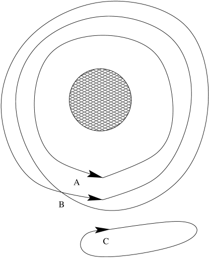
Figure 1: Three examples of transitions that are topologically different. Paths $A$ and $B$ wind around the hold once ($n=1$) and twice ($n=2$) respectively whereas path $C$ does not wind ($n=0$). Path $C$ can be shrunk to a point whereas the others cannot. Each path is said to belong to a different homotopy class. Only paths $A$ and $B$ are affected by the topology of the space. Path $C$ might imagine that it is living in a space with no hole.

An example of the situation described above is the well-known $1+1$ dimensional sine-Gordon model defined by the Lagrangian ${\cal L}_{\rm SG}=\frac{1}{2}(\partial_{\mu}\phi)^{2}-\lambda\cos(\phi)$. Here, the topological current $q_{\mu}=\frac{1}{2\pi}\epsilon_{\mu\nu}\partial^{\nu}\phi$ and is related to the $\phi\rightarrow\phi+2\pi n$ symmetry of the ground state. The well known soliton and antisoliton (kink) solutions are absolutely stable objects with topological charges $Q=\pm 1$. These cannot be recovered by the standard methods of quantum field theory when one starts from the vacuum state $\langle\phi\rangle=0$ and ignores the topology.

In our case an analogous ground state symmetry is realized by the procedure of summation over $l$ in Equation (2), which makes symmetry $\theta\rightarrow\theta+2\pi n$ explicit. Thus, in $1+1$ spatial dimensions we have the analogous stable objects. The fact that we actually consider $3+1$ dimensions means that the objects are not point-like solitons as they are in the sine-Gordon model, but rather, are two-dimensional domain walls with finite surface tension.

3.1 Heavy degrees of freedom

What we have said up to this point is well known. In the sine-Gordon model, the solitons are absolutely stable objects as can be seen by the fact that they are associated with the conserved current $\frac{1}{2\pi}q_{\mu}=\epsilon_{\mu\nu}\partial^{\nu}\phi$ (here, the indices run over the $1+1$ dimensions $z$ and $t$). The conservation is trivial: $\partial^{\mu}q_{\mu}=\frac{1}{2\pi}\epsilon_{\mu\nu}\partial^{\mu}\partial^{\nu}\phi=0$. The corresponding topological charge is $Q=\int q_{t}dz=\frac{1}{2\pi}\int-\partial_{z}\phi(z)dz=\frac{1}{2\pi}(\phi_{z=-\infty}-\phi_{z=+\infty})=n_{-}-n_{+}$ which is described by the winding number $n=n_{+}-n_{-}$. Here, the field is in a vacuum state $\phi_{z=\pm\infty}=2\pi n_{\pm}$ at infinity. Thus, we see that the charge is absolutely conserved and is integral.

In our effective theory (2), we consider an analogous conserved current

$$2\pi q_{\mu}=-i\epsilon_{\mu\nu}{\rm Tr}~{}U^{\dagger}\partial^{\nu}U=\epsilon_{\mu\nu}\partial^{\nu}\sum_{i}\phi_{i}=\epsilon_{\mu\nu}\partial^{\nu}\phi_{S}\,,$$ (19)

where we have introduced the notation $\phi_{S}=\sum_{i}\phi_{i}\sim\eta^{\prime}$ that we shall use later for the isotopical singlet ($\eta^{\prime}$) field. By the same argument, we see that the two dimensional domain walls of the theory (2) are absolutely stable.

In the sine-Gordon model, this is the end of the story: the solitons are absolutely stable. In our effective Lagrangian (2), however, we have neglected the gluon degrees of freedom. In reality, however, the gluon degrees of freedom are not very heavy. Thus, we must consider these extra degrees and look at how they affect the charge conservation. What we find is that, when we account for the extra gluon degrees of freedom, the topology of the fields is no longer restricted to the $\mathop{\rm{}U}(1)$ manifold. These extra degrees of freedom allow the domain walls to continuously deform and to decay so that the ground state exists everywhere.

To see how an extra degree of freedom can change the topology, consider figure 2. Here we have added a third dimension to show that the barrier was actually a peg of finite height. Now that we can move in the extra dimension, we can use this degree of freedom to “lift” the paths over the peg: thus, they are no longer topologically stable. In the QCD analogue, paths $A$ and $B$ represents domain walls (path $C$ would is a trivial closed loop which would relax to a point representing the same vacuum state everywhere with no domain wall.). There is an energy cost to “lift” the path over the barrier and at low temperatures $T\ll\Lambda_{{\rm QCD}}$ there is not enough energy to do this, so classically, the domain walls are stable. It is still possible, however, for the walls to overcome the barrier by tunnelling through the barrier. The tunnelling probability, however, could be low due to the height of the obstacle and hence the lifetime of the walls could be much larger than the $\Lambda_{{\rm QCD}}^{-1}$ scale which one might naïvely expected for standard QCD fluctuations. See Section 5 for details of the dynamics of the gluon fields.

We should also remark that with each winding, the domain walls become more energetic. Walls with a large number of windings either have enough energy to rapidly unwind, or else separate spatially forming several domain walls of winding number $\sim\pm 1$. For this reason, we shall discuss in this paper only the simplest walls which wind once.

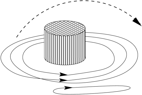
Figure 2: Here we show the same picture as in figure 1 except that we show the third dimension. Here we can see that all the paths are now homotopically equivalent. We can deform the paths by “lifting” them over the obstacle so that we can unwind them. If the paths were strings with some weight, then it would require some energy to “lift” the strings over the obstacle. If this energy was not available, then we would say that, classically, the configurations that wind around the peg are stable. Quantum mechanically, however, the strings could still tunnel through the peg, and so the configurations are unstable quantum mechanically. The probability that one string could tunnel into another configuration would depend on the height of the peg. 

To tie this picture together, consider the formerly conserved current (19) and effective Lagrangian (2) and ask: from where do the phase fields $\phi_{i}$ come? These phases arise from some sort of complex field $\Phi=\rho e^{i\phi_{S}}$. In general, we must consider the dynamics, not only of the phase $\phi_{S}$, but of the component $\rho=|\Phi|$. We assume that this field lives in some sort of Mexican-hat potential with approximate symmetry $\phi_{S}\rightarrow\phi_{S}+\alpha$ and minimum valley where $\langle\rho\rangle=1$. This symmetry is thus spontaneously broken by the vacuum expectation values of the condensate $\langle\Phi\rangle=\exp(i\langle\phi_{S}\rangle)$. To recover the effective Lagrangian: we “integrate” over the “heavy” $\rho$ degree of freedom by setting $\rho=\langle\rho\rangle=1$ equal to its classical expectation value and ignoring the quantum fluctuations about this minimum. This must reproduce the effective potential (2) with the pseudo-Goldstone field $\phi_{S}$ ($\eta^{\prime}$ and $\pi_{i}$ in the real theory). The appropriate Mexican-hat potential reproducing (2) is given in (44).

One can now consider an appropriate generalization of the current (19)

$$2\pi q_{\mu}=-i\epsilon_{\mu\nu}{\rm Tr}~{}\Phi^{\dagger}\partial^{\nu}\Phi=\epsilon_{\mu\nu}\left(-i\rho\partial^{\nu}\rho+\rho^{2}\partial^{\nu}\phi_{S}\right)$$ (20)

which reduces to (19) when we set $\rho=\langle\rho\rangle=1$. Now we have

$$\pi\partial^{\mu}q_{\mu}=\rho\;\epsilon_{\mu\nu}\;\partial^{\mu}\rho\;\partial^{\nu}\phi_{S}$$ (21)

which is no longer conserved as expected. This was only conserved in the effective theory (2) because we integrated out the heavy degrees of freedom by setting $\rho=1$ so that $\partial^{\mu}\rho=0$. Thus, the decay of the domain walls is directly related to the dynamics of the heavy degrees of freedom. We consider this effect in Section 5. The physical object responsible for this behaviour in (2) is the gluon condensate $E\sim\langle G^{2}\rangle$, which is the most essential contribution to the mass $m_{\eta^{\prime}}$ of the $\eta^{\prime}$ particle.

4 Domain walls

In the rest of this paper we limit ourselves with the simplest case $N_{f}=2$ and neglect the difference between $f_{\pi}$ and $f_{\eta^{\prime}}$ which numerically are very close to each other. To describe the basic structure of the QCD domain walls as well as that of axion domain walls we replace the parameter $\theta$ in Equation (2) by a dynamical axion field $\theta\rightarrow N_{f}a=2a$ (this corresponds to the so-called $N=2$ axion model). We also introduce here the following dimensionless phases, $\phi_{S}$ describing the isotopical “singlet” field, and $\phi_{T}$ describing the isotopical “triplet” field. These fields correspond to the dynamical $\eta^{\prime}$ (singlet) and pion $\pi^{0}$ (triplet) fields defined in (1). In principle, there are other dynamical fields corresponding to the remaining $\mathop{\rm SU}(N_{f})$ generators (such as the charged pion fields $\pi^{\pm}$), but one can show that these fields do not contribute to the domain wall background but simply remain in their vacuum states. These fluctuations affect the overall energy density, but do not affect the properties of the domain wall such as the surface tension and so we neglect these in what follows. (See for example [39] where the $N_{f}=2$ case is explicitly considered and $\pi^{\pm}=0$ along the entire domain wall.)

$$\begin{array}[]{rclcrcl}\phi_{S}&=&\phi_{u}+\phi_{d}\,,&&\eta^{\prime}&=&\displaystyle\frac{f_{\pi}}{2\sqrt{2}}\phi_{S}\,,\\[9.0pt] \phi_{T}&=&\phi_{u}-\phi_{d}\,,&&\pi^{0}&=&\displaystyle\frac{f_{\pi}}{2\sqrt{2}}\phi_{T}\,.\end{array}$$ (22)

In what follows we also need to know the masses of the relevant fields in terms of parameters of the effective potential (2):

$$m_{\pi}^{2}=\frac{4M}{f_{\pi}^{2}}\,,\qquad m_{a}^{2}=\frac{4M}{f_{a}^{2}}\left(1-\xi^{2}\right),$$ (23)

and the $\eta^{\prime}$ mass relation

$$m_{\eta^{\prime}}^{2}=\frac{8}{N_{c}^{2}f_{\pi}^{2}}E+\frac{4M}{f_{\pi}^{2}}\,,$$ (24)

follows from (15) with $N_{f}=2$. Here we have neglected all possible mixing terms, and have introduced the following notations

$$M \equiv \frac{M_{u}+M_{d}}{2}=\frac{m_{u}\big{|}\!\langle 0|\bar{\Psi}_{u}\Psi_{u}|0\rangle\!\big{|}+m_{d}\big{|}\!\langle 0|\bar{\Psi}_{d}\Psi_{d}|0\rangle\!\big{|}}{2}\,,$$

$$\xi = \frac{M_{d}-M_{u}}{M_{d}+M_{u}}\approx 0.3\,.$$ (25)

4.1 Domain wall equations

To study the structure of the domain wall we look at a simplified model where one half of the universe is in one ground state and the other half is in another. The fields will orient themselves in such a way as to minimize the energy density in space, forming a domain wall between the two regions. In this model, the domain walls are planar and we shall neglect the $x$ and $y$ dimensions for now. Thus, a complete description of the wall is given by specifying the boundary conditions and by specifying how the fields vary along $z$.

The contribution of the light degrees of freedom to the energy density of a domain wall is given by the following expression

$$\sigma=\int_{-\infty}^{\infty}{\rm d}z\left(\frac{f_{a}^{2}\dot{a}^{2}}{4}+\frac{f_{\pi}^{2}\dot{\phi}_{T}^{2}}{16}+\frac{f_{\pi}^{2}\dot{\phi}_{S}^{2}}{16}+V(\phi_{S},\phi_{T},a)-V_{\rm min}\right)$$ (26)

where the first three terms are the kinetic contribution to the energy and the last term is the potential. The kinetic term is actually a four divergence, but we have assumed the wall to be a stationary solution — hence the time derivatives vanish — and symmetric in the $x$–$y$ plane. The only dependence remaining is the $z$ dependence. Here, a dot signifies differentiation with respect to $z$: $\dot{a}=\frac{{\rm d}a}{{\rm d}z}$.

Now, to find the form of the domain walls, it is convenient to use a form of the potential which follows from (8):

$$V(\phi_{S},\phi_{T},a)=-2M\left(\cos\Bigl{(}\frac{\phi_{S}}{2}+a\Bigr{)}\cos\frac{\phi_{T}}{2}+\xi\sin\Bigl{(}\frac{\phi_{S}}{2}+a\Bigr{)}\sin\frac{\phi_{T}}{2}\right)-E\cos\frac{\phi_{S}}{N_{c}}.$$ (27)

Here we have redefined the fields $\phi_{u}\rightarrow\phi_{u}+a$ and $\phi_{d}\rightarrow\phi_{d}+a$ in order to remove the axion field from the last term $\sim E$ and to insert it into the term $\sim M$. To minimize these equations, we can apply a standard variational principle and arrive at the following equations of motion for the domain wall solutions:

$$\frac{\ddot{a}f_{a}^{2}}{4M} =\cos\!\left(\frac{\phi_{T}}{2}\right)\sin\!\left(\frac{\phi_{S}}{2}+a\right)-\xi\sin\!\left(\frac{\phi_{T}}{2}\right)\cos\!\left(\frac{\phi_{S}}{2}+a\right),$$ (28)

$$\frac{\ddot{\phi_{T}}f_{\pi}^{2}}{8M} =\sin\!\left(\frac{\phi_{T}}{2}\right)\cos\!\left(\frac{\phi_{S}}{2}+a\right)-\xi\cos\!\left(\frac{\phi_{T}}{2}\right)\sin\!\left(\frac{\phi_{S}}{2}+a\right),$$ (29)

$$\frac{\ddot{\phi_{S}}f_{\pi}^{2}}{8M} =\cos\!\left(\frac{\phi_{T}}{2}\right)\sin\!\left(\frac{\phi_{S}}{2}+a\right)-\xi\sin\!\left(\frac{\phi_{T}}{2}\right)\cos\!\left(\frac{\phi_{S}}{2}+a\right)+\frac{E}{MN_{c}}\sin\!\left(\frac{\phi_{S}}{N_{c}}\right),$$ (30)

where the last term of Equation (30) should be understood as the lowest branch of the multivalued function described by Equation (2). Namely, for $\phi_{S}\notin[0,\pi]$, this should be interpreted as $\sin\bigl{(}(\phi_{S}-2\pi l)/N_{c}\bigr{)}$ with the integer $l$ chosen to minimize the potential term $\cos\bigl{(}(\phi_{S}-2\pi l)/{N_{c}}\bigr{)}$. For example, with $\pi\leq\phi_{S}\leq 2\pi$, the last term should be of the form $\sin\bigl{(}(\phi_{S}-2\pi)/N_{c}\bigr{)}$.

Notice the following features: first, the trigonometric terms on the right hand side are of, at most, order $1$; thus the scale for the curvature (or rather, the second derivative) of the domain wall solutions is limited by $f_{a}^{2}/M$ and $f_{\pi}^{2}/M$ etc. In particular, the axion domain wall must have a characteristic scale larger than $m_{a}^{-1}/(1-\xi^{2})$ and the pion domain wall must have a scale larger than $m_{\pi}^{-1}$. The last term in equation governing the $\phi_{S}$ field can potentially be somewhat larger than $1$, hence the smallest scale for the $\phi_{S}$ field is related to the $\eta^{\prime}$ mass. We see immediately that an axion domain wall must have a structure some thirteen orders of magnitude larger than the natural QCD scale and that the $\eta^{\prime}$ field can have structure one order of magnitude smaller than that of the pion field.

4.2 QCD domain walls

Here we consider the most important case of the QCD domain wall solution which exists with or without an axion field. So we now set $a=0$. The equations of motion become:

$$\frac{\ddot{\phi_{T}}f_{\pi}^{2}}{8M} =\sin\!\left(\frac{\phi_{T}}{2}\right)\cos\!\left(\frac{\phi_{S}}{2}\right)-\xi\cos\!\left(\frac{\phi_{T}}{2}\right)\sin\!\left(\frac{\phi_{S}}{2}\right),$$

$$\frac{\ddot{\phi_{S}}f_{\pi}^{2}}{8M} =\cos\!\left(\frac{\phi_{T}}{2}\right)\sin\!\left(\frac{\phi_{S}}{2}\right)-\xi\sin\!\left(\frac{\phi_{T}}{2}\right)\cos\!\left(\frac{\phi_{S}}{2}\right)+\frac{E}{MN_{c}}\sin\!\left(\frac{\phi_{S}}{N_{c}}\right).$$ (31)

For convenience, we shall label the vacuum states using the notation $(\phi_{u},\phi_{d})$. Thus, we have only one physical ground state $(\phi_{u},\phi_{d})=(0,0)$, however, because of the conserved topological current (19), classically stable domain walls can form and interpolate from the ground state $(\phi_{u},\phi_{d})=(0,0)$ along a path which is not homotopic to the null path. To classify the paths we use the redundant notation where $(0,0)$ and $(2\pi,0)$ etc. are considered as different states and we talk about the field interpolating between these states. Keep in mind that this is only a way of classifying the homotopy classes and that in fact all the states represented by $(2\pi n,2\pi m)$ for integers $m$ and $n$ are one in the same vacuum state.

The simplest domain wall is described by a continuous transition from the ground state $(\phi_{u},\phi_{d})=(0,0)$ to the state labelled $(\phi_{u},\phi_{d})=(2\pi,0)$ as described by the vacuum solution Equation (11) with $\theta=2\pi$ (or, equivalently, $l=-1$ in Equation (2)). This wall corresponds to a single winding around the $\mathop{\rm{}U}(1)$ manifold. It is also possible to wind in the opposite sense. To summarize, the two topologically stable domain walls of minimal energy correspond to one winding in each direction and are classified by the transitions from $(\phi_{u},\phi_{d})=(0,0)$ to:

Soliton

$(\phi_{u},\phi_{d})=(2\pi,0)$.

Antisoliton

$(\phi_{u},\phi_{d})=(-2\pi,0)$.

The solutions which wind from $(0,0)$ to $(0,\pm 2\pi)$ are not topologically distinct from these due to the other pion fields and have a higher energy. Note, however, that in the chiral limit $m_{u}=m_{d}$ and $\xi=0$, thus the transitions to $(\phi_{u},\phi_{d})=(0,\pm 2\pi)$ have the same energy and there is a degeneracy. If $m_{u}>m_{d}$, then these transition in $\phi_{d}$ are the minimal energy solutions and the $\phi_{u}$ solutions above become unstable. In reality $m_{d}>m_{u}$, and the transitions to $(\phi_{u},\phi_{d})=(\pm 2\pi,0)$ are the only stable transitions.

The general case of Equations (4.2) cannot be solved analytically and we present the numerical solution of Equation (4.2) in figure 3. In order to gain an intuitive understanding of this wall, we examine the solution in the limit $m_{\pi}\ll m_{\eta^{\prime}}$. In this case, the last term of (4.2) dominates unless $\phi_{S}$ is very close to the vacuum states, $\phi_{S}\simeq 2\pi n$. Thus, the central structure of the $\phi_{S}$ field is governed by the differential equation:

$$\ddot{\phi}_{S}=\frac{8E}{N_{c}f_{\pi}^{2}}\sin\left(\frac{\phi_{S}}{N_{c}}\right).$$ (32)

Now, there is the issue of the cusp singularity when $\phi_{S}=\pi$ because we change from one branch of the potential to another as expressed in Equation (2). By definition, we keep the lowest energy branch, such that the right hand side of Equation (32) is understood to be the function $\sin(\phi_{S}/N_{c})$ for $0\leq\phi_{S}\leq\pi$ and $\sin\bigl{(}(\phi_{S}-2\pi)/N_{c}\bigr{)}$ for $\pi\leq\phi_{S}\leq 2\pi$. However, we notice that the equations of motion are symmetric with respect to the centre of the wall (which we take as $z=z_{0}$), hence $\phi_{S}=\pi$ only at the centre of the wall and not before, so we can simply look at half of the domain, $z\in(-\infty,0]$, with boundary conditions $\phi_{S}=0$ at $z=-\infty$ and $\phi_{S}=\pi$ at $z=0$. The rest of the solution will be symmetric with $\phi_{S}=2\pi$ at $z=+\infty$. Equation (32) with the boundary conditions above has the solution (recall that $\phi_{S}\equiv\phi_{u}+\phi_{d}$)

$$\phi_{S}(z)\equiv\phi_{u}+\phi_{d}=\begin{cases}4N_{c}\tan^{-1}\!\left[\tan\frac{\pi}{4N_{c}}~{}e^{\mu(z-z_{0})}\right],&z\leq z_{0}\\ 2\pi-4N_{c}\tan^{-1}\!\left[\tan\frac{\pi}{4N_{c}}~{}e^{-\mu(z-z_{0})}\right],&z\geq z_{0}\end{cases}$$ (33)

where $z_{0}$ is the position of the centre of the domain wall and

$$\mu\equiv\frac{2\sqrt{2E}}{N_{c}f_{\pi}}\,,\qquad\lim_{m_{q}\rightarrow 0}\mu=m_{\eta^{\prime}}$$ (34)

is the inverse width of the wall, which is equal to the $m_{\eta^{\prime}}$ mass in the chiral limit (see Equation (24)). Thus, we see that the dynamics of the central portion of QCD domain walls is governed by the $\eta^{\prime}$ field. We shall also refer to the $\phi_{S}$ transition (33) which occurs in several places (see for example Section 4.3.2) as the $\eta^{\prime}$ domain wall. The first derivative of the solution is continuous at $z=z_{0}$, but the second derivative exhibits a finite jump.

Before we continue our discussions regarding the structure of QCD domain walls, a short remark is in order: The sine-Gordon equation, which is similar to Equation (32) with a cusp singularity, was first considered in [34] where a solution similar to (33) was presented. There is a fundamental difference, however, between domain walls discussed in [34] and the domain walls we consider here. In [34], the domain walls were constructed as auxiliary objects in order to describe a decay of metastable vacuum states which may exist under the certain circumstances. The walls we discuss here classically stable physical objects where the solutions interpolate between the same vacuum state; their existence is a consequence of the topology of the $\mathop{\rm{}U}(1)$ singlet $\eta^{\prime}$ field. This topology, represented by the exact symmetry $\theta\equiv\theta+2\pi n$ in Equation (2) is a very general property of QCD and does not depend on the specific choice of parameters or functional form of the effective potential. Similar equations and solutions with application to the axion physics were also discussed in [40].

The solution described above dominates on scales where $|z|\leq\mu^{-1}$, however, the isotopical triplet pion transition can only have a structure on scales larger than $m_{\pi}^{-1}\gg\mu^{-1}$ and so the central structure of the $\eta^{\prime}$ wall can have little effect on the pion field. Indeed, we can see that, for $|z|\gg\mu^{-1}$, $\phi_{S}$ is approximately constant with the vacuum values. Making this approximation, we see that the isotopical triplet field is governed by the equation

$$\ddot{\phi}_{T}=2m_{\pi}^{2}\sin\!\left(\frac{\phi_{T}}{2}\right).$$ (35)

This has the same form as (32) and hence the solution is (recall that $\phi_{T}\equiv\phi_{u}-\phi_{d}$)

$$\phi_{T}(z)\equiv\phi_{u}-\phi_{d}=\begin{cases}8\tan^{-1}\!\left[\tan\tfrac{\pi}{8}~{}e^{m_{\pi}(z-z_{0})}\right],&z\ll z_{0}-\mu^{-1},\\ 2\pi-8\tan^{-1}\!\left[\tan\tfrac{\pi}{8}~{}e^{-m_{\pi}(z-z_{0})}\right],&z\gg z_{0}+\mu^{-1},\end{cases}$$ (36)

which is a reasonable approximation for all $z$. Numerical solutions for the $\phi_{S}$ and $\phi_{T}$ fields are shown along with the same solution in terms of the $\phi_{u}$ and $\phi_{d}$ in figure 3. As we can see from the explicit form of the presented solution, the $\eta^{\prime}$ transition is sandwiched in the pion transition. This is a key feature for some applications of this type of the domain wall as discussed in [9] for example.

The contribution to the wall surface tension defined by Equation (26) can be easily calculated analytically in the chiral limit when the analytical solution is known and is given by Equations (33) and (36). Simple calculations leads to the following contribution from the pion and $\eta^{\prime}$ fields.

$$\sigma=\frac{4N_{c}}{\sqrt{2}}f_{\pi}\sqrt{\left\langle\frac{b\alpha_{s}}{32\pi}G^{2}\right\rangle}\,\left(1-\cos\frac{\pi}{2N_{c}}\right)+{\rm O}(m_{q}f_{\pi}^{2})\,.$$ (37)

In case when $m_{q}\neq 0$, an analytical solution is not known, but numerically, $\sigma$ is close to the estimate (37).

\psfrag{eta}{}\psfrag{cz}{\scriptsize$zm_{\eta^{\prime}}$}\psfrag{Pionxxx}{\scriptsize$\phi_{T}(z)$}\psfrag{Etaxxx}{\scriptsize$\phi_{S}(z)$}\psfrag{Phiuxxx}{\scriptsize$\phi_{u}(z)$}\psfrag{Phidxxx}{\scriptsize$\phi_{d}(z)$}\includegraphics[width=208.13574pt]{qcd1.eps}

\psfrag{eta}{}\psfrag{cz}{\scriptsize$zm_{\eta^{\prime}}$}\psfrag{Pionxxx}{\scriptsize$\phi_{T}(z)$}\psfrag{Etaxxx}{\scriptsize$\phi_{S}(z)$}\psfrag{Phiuxxx}{\scriptsize$\phi_{u}(z)$}\psfrag{Phidxxx}{\scriptsize$\phi_{d}(z)$}\includegraphics[width=208.13574pt]{qcd2.eps}

Figure 3: Basic form of the QCD domain walls. Notice that the scale for the pion transition is larger than for the $\eta^{\prime}$ transition and that the width of the $\eta^{\prime}$ wall is set by the scale $m_{\eta^{\prime}}$.

4.3 Axion dominated domain walls

In the previous subsection when the QCD domain walls were discussed, the axion was not introduced as a dynamical field. In this subsection we assume that the axions exist. In this case there are domain walls in which the axion is the dominant player. The introduction of axions, in most cases, makes the domain wall an absolutely stable object. Our case is no exception and the axion model under discussion, (which is the $N=2$ axion models according to the classification [30, 31, 32]) is an absolutely stable object. At the same time it is well-known [41, 38], that stable domain walls can be a cosmological disaster. We do not address in this paper the problem of avoiding a domain wall dominated universe. Rather, we would like to describe some new elements in the structure of axion domain walls, which were not previously discussed.

The first and most natural type of the axion domain wall was discussed by Huang and Sikivie [39] who neglected the $\eta^{\prime}$ field in their construction. We shall refer to this wall as the Axion-Pion domain wall ($a_{\pi}$). As shown in [39], it has a width of the scale $\sim m_{a}^{-1}\gg\Lambda_{{\rm QCD}}^{-1}$ for both the axion and $\pi$ meson components. As Huang and Sikivie expected, the $\eta^{\prime}$ plays a very small role in this wall. In what follows we include a discussion of this type of domain wall for the completeness.

\psfrag{eta}{}\psfrag{caz}{\scriptsize$zm_{a}$}\psfrag{Axion}{\scriptsize$a(z)$}\psfrag{Pion}{\scriptsize$\phi_{T}(z)$}\psfrag{Eta}{\scriptsize$\phi_{S}(z)$}\includegraphics[width=238.49231pt]{ap1.eps}

Figure 4: Basic form of the $a_{\pi}$ domain wall. Notice that all the fields have a structure on the scale of $m_{a}^{-1}$ and that the isotopical singlet fields plays a very small role.

Our original result is to description a new type of the axion domain wall in which the $\eta^{\prime}$ field is a dominant player. We shall call this new solution the Axion-Eta’ domain wall ($a_{\eta^{\prime}}$). This new type of the domain wall was considered for the first time in [9] as a possible source for galactic magnetic fields in early universe. In what follows we give a detail description of the solution for the $a_{\eta^{\prime}}$ wall. Here we want to mention the fundamental difference between the $a_{\pi}$ wall discussed in [39] and the $a_{\eta^{\prime}}$ wall introduced in [9].

Unlike the $a_{\pi}$ wall which has structure only on the huge scale of $m_{a}^{-1}$, the $a_{\eta^{\prime}}$ wall has nontrivial structure at both the axion scale $m_{a}^{-1}$ as well as at the QCD scale $m_{\eta^{\prime}}^{-1}\sim\Lambda_{\rm QCD}^{-1}$. The reason for this is that, in the presence of the non-zero axion field (which is equivalent to a non-zero $\theta$ parameter), the pion mass is efficiently suppressed due to its Goldstone nature, thus the pion field follows the axion field and has a structure on the same $m_{a}^{-1}$ scale. The $\eta^{\prime}$, however, is not very sensitive to $\theta$ and so it remains massive.

Again, the $a_{\eta^{\prime}}$ solution has a sandwich structure with the singlet transition occurring at the centre of the wall. One can adopt the viewpoint that the $a_{\eta^{\prime}}$ domain wall is an axion domain wall with a QCD domain wall sandwiched in the centre. This phenomenon is critical for applications involving the interaction of domain walls with strongly interacting particles. Indeed, there is no way for the $a_{\pi}$ wall to trap any strongly interacting particles, like nucleons, because of the huge difference in scales; the $a_{\eta^{\prime}}$ wall, however, has a QCD structure and can therefore efficiently interact with nucleons on the QCD scale $\Lambda_{\rm QCD}^{-1}$. Regarding the wall tension (26), it is dominated by the axion physics and thus has the same order of magnitude for both types of the axion domain walls which is proportional to $\sigma\sim M/m_{a}\sim f_{a}f_{\pi}m_{\pi}$ as found in [39].

4.3.1 Axion-pion domain wall

The solution discussed by Huang and Sikivie corresponds to the transition $(a,\phi_{u},\phi_{d}):\;(0,0,0)\rightarrow(\pi,\pi,-\pi)$, i.e., by a transition in the axion and pion fields only. This transition describes the $a_{\pi}$ wall. Indeed, in terms of $(a,\phi_{S},\phi_{T})$ this transition corresponds to a nontrivial behaviour of the axion and triplet pion component $\phi_{T}$ of the $\phi_{u},\phi_{d}$ fields: $(a,\phi_{S},\phi_{T}):\;(0,0,0)\rightarrow(\pi,0,2\pi)$. The other transition (the $a_{\eta^{\prime}}$ wall) corresponds to the transition $(a,\phi_{u},\phi_{d}):\;(0,0,0)\rightarrow(-\pi,\pi,\pi)$ in which the singlet $\eta^{\prime}$ field is dominant: $(a,\phi_{S},\phi_{T}):\;(0,0,0)\rightarrow(-\pi,2\pi,0)$. It will be considered later on.

Huang and Sikivie discussed the solution to this wall in the limit where the $\eta^{\prime}$ field is extremely massive and hence they neglected its role. It can be integrated out which effectively corresponds to fixing it $\eta^{\prime}(z)=0$. Indeed, if we simply fix $\eta^{\prime}(z)=0$ in our equations, then we reproduce their solution. When $E$ is large, then $m_{\pi}\ll m_{\eta^{\prime}}$ as Huang and Sikivie assumed, the effects of the $\eta^{\prime}$ particle can be neglected and the solution for the the axion and pion fields presented in [39] is valid for the boundary conditions described above. We plot this numerical solution which includes the $\eta^{\prime}$ effects in figure 4. As announced above, the $a_{\pi}$ solution has the only scale of $\sim m_{a}^{-1}$ for both components, axion as well as the pion field $\sim\phi_{T}$. The $\eta^{\prime}$ field remains close to the its vacuum value and only slightly corrects the solution.

4.3.2 Axion-eta’ domain wall

Having looked at the solution of the $a_{\pi}$ wall, we now investigate the structure of the $a_{\eta^{\prime}}$ domain wall which is a new solution. This solution corresponds to the transition $(a,\phi_{u},\phi_{d}):\;(0,0,0)\rightarrow(\pi,\pi,\pi)$. Now the singlet $\eta^{\prime}$ field undergoes a transition instead of the triplet pion field: $(a,\phi_{S},\phi_{T}):\;(0,0,0)\rightarrow(-\pi,2\pi,0)$. As we discussed above, the singlet field never becomes massless, and therefore, a new structure at the QCD scale $\sim\Lambda_{{\rm QCD}}^{-1}$ emerges in sharp contrast to the well-studied $a_{\pi}$ domain wall [39] where no such structure appears. We should note that the potential (27) has the same vacuum energy at $\phi_{S}=0$ as well as at $\phi_{S}=2\pi$ due to the change of $\phi_{S}$ field to the lowest energy branch at $\phi_{S}=\pi$ as described by Equation (2). Therefore, this domain wall interpolates between two degenerate states, and thus, like the $a_{\pi}$ domain wall [39], the solution under these considerations is absolutely stable.

For $|z|\gg\mu^{-1}$, the last term in (30) is negligible and so the solution behaves like the $a_{\pi}$ wall. What happens is that, away from the wall, the axion field dominates and shapes the wall as it does in with the $a_{\pi}$ solution. Again, the pion mass is suppressed and $\phi_{S}\approx 0$. As $z\sim\mu^{-1}$ however, the last term of (4.2) starts to dominate the behaviour. At this point, the $a_{\eta^{\prime}}$ wall undergoes a sharp transition similar to the QCD domain wall described by (33). We plot this solution along with a blowup in figure 5. Notice also, that the singlet field cancels the effects of the axion near the center of the wall, and so the pion field becomes massive again as it undergoes its transition.

\psfrag{eta}{}\psfrag{cza}{\scriptsize$zm_{a}$}\psfrag{cze}{\scriptsize$zm_{\eta^{\prime}}$}\psfrag{Axion}{\scriptsize$a(z)$}\psfrag{Pion}{\scriptsize$\phi_{T}(z)$}\psfrag{Eta}{\scriptsize$\phi_{S}(z)$}\includegraphics[width=208.13574pt]{ae1.eps}

\psfrag{eta}{}\psfrag{cza}{\scriptsize$zm_{a}$}\psfrag{cze}{\scriptsize$zm_{\eta^{\prime}}$}\psfrag{Axion}{\scriptsize$a(z)$}\psfrag{Pion}{\scriptsize$\phi_{T}(z)$}\psfrag{Eta}{\scriptsize$\phi_{S}(z)$}\includegraphics[width=208.13574pt]{ae2.eps}

Figure 5: Basic form of the $a_{\eta^{\prime}}$ domain walls with a closeup where the axion field $a\approx\pi/2$. Notice that the large scale structure is similar to that of the $a_{\pi}$ wall, but that there is also a small scale structure on the scale of $m_{\eta^{\prime}}$. Near the centre of the wall, the pion regains its mass and undergoes a transition on the scale of $m_{\pi}$.

5 Decay of the QCD domain walls

We do not have much new to say regarding the generalities of domain walls, nor do we have a resolution for the general problem of avoiding a domain wall dominated universe. We have nothing new to say regarding the stability or evolution of axion domain walls [42]–[49] (which were also discussed in the previous sections), see [50] and references therein for a recent review on the subject. We refer the reader to the nice text book [38] for general discussion about domain walls, other topological defects and their role in the early universe. This section is devoted specifically to the QCD domain walls discussed in Section 4.2.

Up to now, we have treated the domain walls as topologically stable objects. If we only consider the low energy degrees of freedom present in the effective theory (2) then this is certainly the case as discussed in Section 3. We shall also argue that this picture of classically stable domain walls is correct in the appropriate large $N_{c}=\infty$ and chiral $m_{q}=0$ limit. In reality, however, one must consider the heavy degrees of freedom that were integrated out to obtain (2). For finite $N_{c}$, one finds that QCD domain walls (not axion domain walls) are unstable on the quantum level due to a tunnelling mode of decay as described in Section 3.1. We estimate the relevant life-time of these walls with respect to this quantum transition and show that, although the walls don’t live long on a cosmological scale, exponential suppression of the tunnelling decay mode may result in the lifetime of the walls being much larger than the QCD scale $\Lambda_{{\rm QCD}}^{-1}$. We argue that this exponential suppression remains in the large $N_{c}$ limit where we have theoretical control, and may also occur numerically for physical values of the parameters. Therefore, these walls do not pose a cosmological problem as one might naïvely suspect.

Even though QCD domain walls are ultimately unstable, they may still play an important role in physical processes with timescales comparable to the lifetime of the walls. QCD domain walls are not likely to exist today, however, they may play an important role shortly after the QCD phase transition in the evolution of the early universe, or in heavy ion collisions after the transition from a quark-gluon plasma to the hadronic phase when system cools. In these cases, QCD domain walls with a finite lifetime may play an important role. Indeed, according to the standard theory of cosmological phase transitions [51, 38], if, below a critical temperature $T_{c}$, the potential develops a number of degenerate minima, then the choice of minima will depend on random fluctuations in fields. The minima that the fields settle to can be expected to differ in various regions space. If neighbouring volumes fall into different minima, then a kink (domain wall) will form as a boundary between them. The relevant question becomes: “Is the lifetime of QCD domain walls large enough to be of physical interest?” In what follows, we hope to convince the reader that the answer to this question may in fact be: “Yes!”.

5.1 Estimating the decay rate

In the following, we estimate the lifetime of the QCD domain walls due to a tunnelling process whereby a hole forms in the domain wall and expands, consuming the wall. A quantitative calculation of this rate is presently beyond our control, but we can estimate the magnitudes of the effect through a semi-classical approximation. In Section 5.5 we shall argue that these approximations are valid asymptotically in the large $N_{c}$ limit and that the decay rate is exponentially suppressed.

The decay mechanism is due to a tunnelling process which creates a hole in the domain wall which connects the $(\phi_{u},\phi_{d})=(0,0)$ domain on one side of the wall to the $(\phi_{u},\phi_{d})=(2\pi,0)$ domain on the other (see Equation (11)). Passing through the hole, the fields remain in the ground state. This lowers the energy of the configuration over that where the hole was filled by the domain wall transition by an amount proportional to $R^{2}$ where $R$ is the radius of the hole. The hole, however, must be surrounded by a string-like field configuration. This string represents an excitation in the heavy degrees of freedom and thus costs energy, however, this energy scales linearly as $R$. Thus, if a large enough hole can form, then it will be stable and the hole will expand and consume the wall.

This process is commonly called quantum nucleation and is similar to the decay of a metastable wall bounded by strings, and we use a similar technique to estimate the tunnelling probability. The idea of the calculation was suggested by Kibble [53], and has been used many times since then (see the textbook [38] for a review). The most well known example of such a calculation is the calculations of the decay rate in the so-called $N_{PQ}=1$ axion model where the axion domain wall become unstable for a similar reason due to the presence of axion strings [45]–[50]. However, as was emphasized in [54], the existence of strings as the solutions to the classical equations of motion is not essential for this decay mechanism (see below). Some configurations, not necessarily the solutions of classical equations of motion, which satisfy appropriate boundary conditions, may play the role played by strings in the $N_{PQ}=1$ axion model.

To be more specific, let us consider a closed path starting in the first domain with $(\phi_{u},\phi_{d})=(0,0)$, which goes through the hole and finally returns back to the starting point by crossing the wall somewhere far away from the hole. The phase change along the path is clearly equals to $\phi_{u}+\phi_{d}=2\pi$. Therefore, the absolute value of a field which gives the mass to the $\eta^{\prime}$ field (the dominant part of the domain wall) has to vanish at some point inside the region encircled by the path. By moving the path around the hole continuously, one can convince oneself that there is a loop of a string-like configuration (where the absolute value of a relevant field vanishes such that the $\eta^{\prime}$ singlet phase is a well defined) enclosing the hole somewhere. In this consideration we did not assume that a hole, or string enclosing the hole, are solutions of the equations of motion. They do not have to be solutions.

However, if we want to describe the hole nucleation semi-classically [53, 38], then we should look for a corresponding instanton which is a solution of Euclidean (imaginary time, $t=i\tau$) field equations, approaching the unperturbed wall solution at $\tau\rightarrow\pm\infty$. In this case the probability $P$ of creating a hole with radius $R$ per area $S$ per time $T$ can be estimated as follows [53, 56, 57]:

$$\frac{P}{ST}\sim\left[\sqrt{\frac{S_{0}}{2\pi}}\right]^{3}e^{-S_{0}}\times{\rm Det}\,,$$ (38)

where $S_{0}$ is the classical instanton action; Det can be calculated by analyzing small perturbations (non-zero modes contribution) about the instanton, (see [57] for an explanation of the meaning of this term) and will be estimated using dimensional arguments; and $\bigl{(}\sqrt{S_{0}/(2\pi)}\bigr{)}^{3}$ is the contribution due to three zero modes describing the instanton position.

If the radius of the nucleating hole is much greater than the wall thickness, we can use the thin-string and thin-wall approximation. (The critical radius $R_{c}$ will be estimated later and this approximation justified). In this case, the action for the string and for the wall are proportional to the corresponding worldsheet areas [53],

$$S_{0}=4\pi R^{2}\alpha-\frac{4}{3}\pi R^{3}\sigma\,.$$ (39)

The first term is the energy cost of forming a string: $\alpha$ is the string tension and $4\pi R^{2}$ is its worldsheet area. The second term is energy gain by the hole over the domain wall: $\sigma$ is the wall tension and $4/3\pi R^{3}$ is its worldsheet volume. The world sheet of a static wall lying in the $x$-$y$ plane is the three-dimensional hyperplane $z=0$. In the instanton solution, this hyperplane has a “hole” which is bounded by the closed worldsheet of the string.

Minimizing (39) with respect to $R$ we find the critical radius

$$R_{c}=\frac{2\alpha}{\sigma}\,,\qquad S_{0}=\frac{16\pi\alpha^{3}}{3\sigma^{2}}\,.$$ (40)

The lorentzian evolution of the hole after nucleation can be found by making the inverse replacement $\tau\rightarrow-it$ from Euclidean to Minkowski space-time. The hole expands with time as $x^{2}+y^{2}=R^{2}+t^{2}$, rapidly approaching the speed of light.

To estimate the appropriate string and wall tensions, we must step back from the effective theory (2) and include the heavy degrees of freedom that allow the fields to tunnel. Unfortunately, to provide a well justified estimate of these parameters in standard QCD is very difficult because we do not know how to quantitatively include the effects of the heavy degrees of freedom. We shall argue, however, that we regain this theoretical control in the chiral and large $N_{c}$ limits. We postpone this discussion until Section 5.2, but we summarize the $N_{c}$ dependence of these parameters here:

$$N_{c}\lesssim\alpha\,,\qquad\sqrt{N_{c}}\lesssim\>\sigma\,.$$ (41)

These lower bounds for the string tension $\alpha$ and wall tension $\sigma$ are well justified. For our argument, however, we need an upper bound on the wall tension. As we shall argue later, we expect that the lower bound for $\sigma$ in (41) is actually the upper bound and that:

$$\sigma\sim\sqrt{N_{c}}\,.$$ (42)

However, there is some speculation about the correct upper bound and one might argue that that the upper bound could be of order $N_{c}$. While we strongly suspect that (42) is correct, we cannot prove this and thus consider the possibility of larger $\sigma$.

In either case, from (40) we see that, in the large $N_{c}$ limit, the probability of producing a hole (38) is exponentially suppressed by the factor of at least $e^{-S_{0}}\sim e^{-N_{c}}$ in the case of $\sigma\sim N_{c}$ (In this case, our semiclassical estimate of $S_{0}$ is not numerically justified, however, we believe that it is parametrically still valid as we shall discuss in Section 5.5). We believe, however, that (42) holds and thus that the actual suppression is much stronger

$$e^{-S_{0}}\sim e^{-N_{c}^{2}}\,.$$ (43)

The only way to kill the exponential suppression is to arrange for $\sigma>N_{c}^{3/2}$ which, as we shall discuss, has no phenomenological or theoretical support. Thus, in the limit $N_{c}\rightarrow\infty$, we believe that no tunnelling is supported and the domain walls become stable. In Section 5.6 we shall extrapolate these results to the $N_{c}=3$ limit and, although we lose the theoretical control gained in the large $N_{c}$ limit, we argue that the qualitative picture might remain the same.

5.2 Heavy degrees of freedom

As discussed in Section 3.1, we cannot properly discuss tunnelling with Equation (2) where the gluon degrees of freedom are integrated out and replaced by their vacuum expectation values: such a theory cannot describe the strings which are responsible for the domain wall decay described in Section 5.1. Instead, we must take one step back and describe the dynamics of the gluon condensate by considering the original Lagrangian [12, 13] which includes the complex gluon degrees of freedom $h$. In this effective theory, the complex gluonic field will sit in a Mexican-hat potential with $|\langle h\rangle|=$ const. The string represents a localized region about which $h=0$. In the effective theory (2) this represents a singularity, but here the singularity is allowed, although it is energetically costly. The string tension is associated with the energy cost required to form the string and this is directly related to the height of the peak of the Mexican-hat potential.

The effective potential of the original Lagrangian [12, 13] which includes the complex gluonic degrees of freedom $h$ is given by:

$$V(\theta,h,U)=\left(\frac{h}{4N_{c}}\log\left[\left(\frac{h}{2eE}\right)^{N_{c}}\frac{{\rm Det}\,U}{e^{-i\theta}}\right]-\tfrac{1}{2}{\rm Tr}\,MU\right)+\text{H.c.}$$ (44)

This satisfies all the conformal and chiral anomalous Ward identities, has the correct large $N_{c}$ behaviour etc. (see [12, 13, 34] for details). Integrating out the heavy $h$ field will bring us back to Equation (2). (It is interesting to note that the structure of Equation (44) is quite similar in structure to the effective potential for SQCD [11] and gluodynamics [58].)

Let us stop for a moment to consider the form of this potential. When we integrate out the heavy gluon degrees of freedom, we replace $h$ with its vacuum expectation value $\langle h\rangle$. The vacuum expectation value of the $h$ is given by

$$\langle h\rangle=2E\exp\bigl{(}-i\sum\phi_{i}/N_{c}\bigr{)}=2Ee^{-i\phi_{S}/N_{c}}$$ (45)

such that (44) becomes

$$V(U)\Big{|}_{\genfrac{}{}{0.0pt}{1}{\!\!\!\!\!\theta=0}{h=\langle h\rangle}}=-E\cos\frac{\sum\phi_{i}}{N_{c}}-\sum M_{i}\cos\phi_{i}\,,$$ (46)

in agreement with (8). With $h$ fixed at its vacuum expectation value, the singlet combination $\phi_{S}=\sum{\phi_{i}}$ exhibits the $\mathop{\rm{}U}(1)$ topology described above and our domain walls are stable. Now, however, we allow the gluon condensate to fluctuate. We parameterize these fluctuations in polar coordinates by a radial component $\rho$, and an angular component $\zeta$:

$$h=\rho e^{i\phi_{\zeta}}\langle h\rangle=\rho\exp\left(i\frac{\zeta}{f_{\zeta}}\right)\langle h\rangle\,.$$ (47)

Here $f_{\zeta}$ is the decay constant and $\phi_{\zeta}$ is the dimensionless phase angle. The fields $\rho$ and $\zeta$ are both heavy, real, physical fields. In the large $N_{c}$ limit, their masses are much heavier than the pion or $\eta^{\prime}$ masses: $m_{\zeta}\sim m_{\rho}\gg m_{\eta^{\prime}}$. The role of the $\zeta$ field will be important in explaining the physics of the cusp singularities in (2) and will be discussed in Section 5.4. For now we set $\theta$ and $\phi_{\zeta}$ to zero. In terms of the remaining physical fields, the potential $V$ becomes

$$V(\rho,\phi_{S})=+E\rho\bigl{(}\log\rho-1\bigr{)}\cos\frac{\phi_{S}}{N_{c}}\,,$$ (48)

where we have neglected the terms proportional to $M$ since they only contribute a constant offset due to the $\phi_{T}$ field. For an early phenomenological discussion of the potential (48) without the $\phi_{S}$ fields, see [59].

Now the combined degrees of freedom $\rho$ and $\phi_{S}$ are no longer restricted to the circle $\rho=1$ as they were in the effective theory (2). The $\mathop{\rm{}U}(1)$ topology is no longer a constraint of the fields and thus, the walls are not topologically stable. Instead, the restriction of $\rho\approx 1$ is dynamical, and made by a barrier at $h=0$. Thus, with these degrees of freedom, the fields parameterize the plane, however, the potential is that of a tilted Mexican-hat with a barrier at $h=0$. The barrier is high enough that a domain wall interpolating around the trough of the hat is classically stable. If the barrier were infinitely high as we assumed when we fixed $\rho=1$ as we did in (2), then the $\phi_{S}$ field could wind around the barrier and would be topologically stable. With a finite barrier, however, the field can tunnel through the barrier as described above. This situation is analogous to the case of the string and peg shown in figure 2. We show a more accurate picture of the barrier (48) in figure 6. The relative heights of the the peak and troughs are given below:

$$\Delta V_{\rm Peak} = \Delta V_{1}+\Delta V_{2}=E\sim N_{c}^{2}\,,$$ (49)

$$\Delta V_{1} = E\cos\frac{\pi}{N_{c}}\sim N_{c}^{2}\,,$$ (50)

$$\Delta V_{2} = E\left(1-\cos\frac{\pi}{N_{c}}\right)\sim 1\,.$$ (51)

We have emphasised the $N_{c}$ dependence here because the effective theories are really only well justified in the large $N_{c}$ limit.

\psfrag{BB}{$\Delta V_{1}\sim N_{c}^{2}$}\psfrag{CC}{$\Delta V_{2}\sim 1$}\psfrag{phi1}{$\phi_{S}=\pi$}\psfrag{phi2}{$\phi_{S}=0$}\includegraphics[width=433.62pt]{hat1.eps}

Figure 6: Profile of the “Mexican-hat” potential (48). The slice is made along the axis through $\phi_{S}=\pi$ to the left and $\phi_{S}=0$ to the right. The trough of the potential lowers from the cusp at $\rho=1$, $\phi=\pi$ where $V=-E\cos(\pi/N_{c})$ down to the vacuum state $V_{\rm min}=-E$. The hump where $V=0$ is at the origin is where $h=\rho\exp(i\phi_{S}/N_{c})=0$ and hence the singlet field $\phi_{S}$ can have any value at this point. It is by passing across this point that a QCD domain wall can tunnel and a hole can form. The important qualitative features of this potential are the height of the central peak $\Delta V_{\rm Peak}$ (49), the relative heights of the cusp to the peak $\Delta V_{1}$ (50) and the trough to the cusp $\Delta V_{2}$ (51).

The most important property of the potential is the following: The absolute minimum of the potential in the chiral limit corresponds to the value $V_{\rm min}=-E$ which is the ground state of our world with $\rho=1$ and $\phi_{s}=0$. At the same time, the maximum of the potential (2), where one branch changes to another one is $V=-E\cos(\pi/N_{c})$ where $\phi_{S}=\pi$ (we are still taking $\theta=0$). This corresponds to the point $\rho=1$ and $\phi_{S}=\pi$ in the potential (48). Thus, the trough of the Mexican-hat is given where $h=\langle h\rangle$, i.e. at radius $\rho=1$ and the maximum $V=-E\cos(\pi/N_{c})$ of the potential (2) is exactly the barrier through which the $\eta^{\prime}$ field interpolates to form the QCD domain wall. It is important to note that the height of the barrier for the potential (2) is numerically is quite high $\sim E(1-\cos\frac{\pi}{N_{c}})$, but vanishes in large $N_{c}$ limit. Indeed, in this limit, the peak of the barrier is degenerate with the absolute minimum $V_{\rm min}=-E$ of the potential as it should be. The height of this barrier describes how much the Mexican-hat is tilted.

The other important property of the potential (48) is its value where the singlet phase $\sum\phi_{i}$ is not well defined at the peak of the Mexican-hat. From (48) it is clear that this occurs for $h=0$. It is this peak of the Mexican-hat in figure 6 (or the peg in figure 2) that classically prevents $\rho\rightarrow 0$ and that makes the QCD domain wall classically stable. When a hole tunnels through the wall, it must be surrounded by a “string” where the field passes through the region $h=0$. The height of the peak thus contributes to the energetic cost of creating such a string (and hence the hole). The potential (48) vanishes at the centre of the string $V(h=0)=0$, which implies that the barrier at $h=0$ is quite high: $\Delta V_{\rm Peak}=E$. As expected, the barrier at $h=0$ should be order of $E\sim N_{c}^{2}$ in contrast with the barrier to the $\eta^{\prime}$ domain wall where one expects a suppression by some power of $N_{c}$. We also note that the total number of distinct classically stable solutions can be estimated from the condition that $\cos(\pi k/N_{c})>0$ where the barrier for the $\eta^{\prime}$ field is still lower than the peak $h=0$. Thus, $-N_{c}/2<k<N_{c}/2$ where $k$ labels the winding number of the solution. Thus we see that for $N_{c}\leq 2$ there is no admissible classically stable solution, but for $N_{c}\geq 3$ classically stable solutions are allowed. In our model with potential (48) we see explicitly that, for $N_{c}=3$, there is one classically stable domain wall while for $N_{c}=2$ there are no classically stable solutions.

5.3 String and wall tensions

In order to make the semi-classical estimates of the decay rate (see Equations (38) and (40)) we must estimate the string tension $\alpha$ and the wall tension $\sigma$. We start with the string tension $\alpha$.

Within the effective theory (44) true strings are not supported because the $\mathop{\rm{}U}(1)$ symmetry is broken by the anomaly. In the large $N_{c}$ limit, however, this symmetry is restored (and the $\eta^{\prime}$ becomes massless). Thus, it makes sense to consider global $\mathop{\rm{}U}(1)$ strings in the large $N_{c}$ limit. To properly estimate $\alpha$ at finite $N_{c}$ one must numerically minimizes the energy of a configuration with a domain wall bounded by a string-like configuration. This could be done numerically, but is beyond the scope of the present paper. In the large $N_{c}$ limit, the estimates presented here become reliable.

To estimate the string tension $\alpha$, we first consider an isolated global string in a flat Mexican-hat potential

$${\mathcal{L}}=\frac{1}{2}\partial_{\mu}\Phi^{*}\partial^{\mu}\Phi-V(|\Phi|)\,,$$ (52)

where $\Phi$ is a generic complex scalar field that will be identified with the glue-ball field $h$ discussed in Section 5.2. To match $V(|\Phi|)$ with (44) we must take the limit $N_{c}\rightarrow\infty$ so that the $\mathop{\rm{}U}(1)$ symmetry $\Phi\rightarrow e^{i\alpha}\Phi$ (equivalently $h\rightarrow e^{i\alpha}h$) is restored. In this case, a string lying along the $z$-axis with winding number $n$ will be described by the complex field configuration

$$\Phi(r,\theta)=\rho(r,\theta)e^{i\phi(r,\theta)}=\rho(r)e^{in\theta}=\rho(r)\exp\left(in\tan^{-1}\frac{y}{x}\right)$$ (53)

in the $x$-$y$ plane. The exact radial dependence $\rho(r)$ will be such as to minimize the energy density along the string and will minimize the energy density

$$\alpha = \iint\left(\frac{1}{2}\partial_{i}\rho\partial_{i}\rho+\frac{1}{2}\rho^{2}\partial_{i}\phi\partial_{i}\phi+V(\rho)-V_{\mathrm{min}}\right)\mathrm{d}x\mathrm{d}y\,,$$ (54)

$$= 2\pi\int\left(\frac{1}{2}\left(\frac{\mathrm{d}\rho}{\mathrm{d}r}\right)^{2}+\frac{n^{2}\rho^{2}}{2r^{2}}+V(\rho)-V_{\mathrm{min}}\right)r\mathrm{d}r\,.$$ (55)

We have assumed here that the fields $\rho$ and $\phi$ are canonically normalized.

Within some radius $r_{s}$, the radial dependence of the string will vary from $0$ to $\langle\rho\rangle$ and there will be a core energy contribution to the string tension

$$\alpha_{0}=\pi r_{s}^{2}V_{0}\,,$$ (56)

where $V_{0}$ represents an average core energy. Far away from the string, $\rho$ will assume its vacuum expectation value and the total string tension (energy density per unit length) will be

$$\alpha\sim\alpha_{0}+\pi\int_{r_{s}}^{R}\frac{n^{2}\langle\rho\rangle^{2}}{r}\mathrm{d}r\sim\alpha_{\mathrm{core}}+\pi n^{2}\langle\rho\rangle^{2}\log R\,,$$ (57)

where we have absorbed all contributions from the region of size $r_{s}$ into the constant $\alpha_{\mathrm{core}}$. For an isolated string, the string tension is infinite, but in most cases, the lateral extent of the string is limited by some upper radius $R$ that must be determined by the dynamics of the strings. In our case, the string is embedded in the end of a domain wall, so the relevant scale for $R$ will be the wall thickness.

Far from the core of the string, the only degree of freedom is the dimensionless phase $\phi$:

$$\Phi=\langle\rho\rangle e^{i\phi}\,.$$ (58)

Thus, the kinetic term is

$$\frac{1}{2}\langle\rho\rangle^{2}\partial_{\mu}\phi\partial^{\mu}\phi\,.$$ (59)

The normalization of the field $\rho$ is such that this term reduces to the appropriate canonical kinetic term for the appropriate Goldstone field described by Equation (52). In our case, the string is composed of the $\eta^{\prime}$ field and the relevant phase $\phi$ interpolates from $0$ to $2\pi$ connecting the two sides of the QCD domain wall. For this $\eta^{\prime}$ string, the the relevant phase is $\phi=2\eta^{\prime}/(f_{\eta^{\prime}}\sqrt{N_{f}})$ is given in (1): thus $\langle\rho\rangle^{2}=N_{f}f_{\eta^{\prime}}^{2}/4$, and the tension is:

$$\alpha\sim\alpha_{\mathrm{core}}+\frac{\pi}{4}N_{f}f_{\eta^{\prime}}^{2}n^{2}\log R\sim\alpha\sim\alpha_{\mathrm{core}}+\frac{\pi}{2}f_{\pi}^{2}\log R\,,$$ (60)

where we have set $N_{f}=2$ and $n=1$ (single winding) in the last equation, as we have been doing.

To determine $\alpha_{\mathrm{core}}$, one must actually minimize the string tension. This requires full knowledge of the potential $V(\rho)$ and the nature of the field $\rho$. We do not have this information. In general, however, we expect that the scale of the core is set by the mass of the heavy field $\rho$

$$r_{s}\sim m_{\rho}^{-1}\sim 1\,,$$ (61)

and thus, in the large $N_{c}$ limit, the string core size becomes much smaller than the domain wall thickness (34)

$$r_{s}\sim m_{\rho}^{-1}\sim 1\ll\mu^{-1}\sim m_{\eta^{\prime}}^{-1}\sim\sqrt{N_{c}}\,,$$ (62)

so one can think of the string as embedded in the edge of the domain wall. In this environment, the outer radius of the string $R$ is the same order as the thickness of the domain wall. This justifies the approximation of the string tension (60) as that of a free string with outer radius $R$: if the string core had been of comparable size to the domain wall, then this approximation would be inaccurate, and we would have had to minimize the energy of the combined system of a domain wall bounded by a string. This situation is much more difficult to solve because the “string” would no longer have cylindrical symmetry.

Unlike the tension of a global string, which has a logarithmic contribution from the bulk (60), the domain wall tension (c.f. Equation (26) come exclusively from the core dynamics. Due to the quadratic kinetic terms, there is an equipartition of energy and the tension is essentially

$$\sigma\sim\Delta zV_{0}\,,$$ (63)

where $\Delta z$ is the wall thickness and $V_{0}\sim V_{\mathrm{core}}-V_{\mathrm{min}}$ is the average potential energy near the core. For most domain walls, the thickness is governed by the mass of the relevant field. Thus, for QCD domain wall tension, we have the following contributions from the pion and $\eta^{\prime}$ transitions respectively (see potential (27)):

$$\sigma_{\pi} \sim m_{\pi}^{-1}2M\sim m_{\pi}^{-1}m_{q}|\langle\bar{\Psi}\Psi\rangle|\sim f_{\pi}^{2}m_{\pi}\,,$$ (64)

$$\sigma_{\eta^{\prime}} \sim m_{\eta^{\prime}}^{-1}E\left(1-\cos\frac{\pi}{N_{c}}\right)\sim\frac{E}{N_{c}^{2}m_{\eta^{\prime}}}\,,$$ (65)

which agree qualitatively with the precise calculations (37). Thus, in the chiral limit $m_{q}\rightarrow 0$, only the $\eta^{\prime}$ contribution remains relevant. Numerically, even with finite quark masses, the $\eta^{\prime}$ contribution is much larger than the pion contribution. There is another contribution, however, due to heavy degrees of freedom which we estimate in the next section.

5.4 Cusps

As was emphasized in [60] for supersymmetric QCD, the presence of a cusp singularity in the effective potential (2) can indicate that heavy degrees of freedom are playing a role in the physics. As far as the low energy degrees of freedom are concerned, (the pions and $\eta^{\prime}$), the effective potential (2) is valid on the scales associated with these degrees of freedom. If we were to properly include the heavy degrees of freedom, we would find that the cusps are actually smooth, but only on scales comparable to the mass of the heavy particles $m_{h}\gg m_{\pi}$. In the centre of the domain wall, where the potential has the cusp, what is really happening is that the heavy fields are making a rapid transition with a scale length of $\Delta z\sim m_{h}^{-1}$.

Analogously to [60], the contribution of this heavy transition to the domain wall tension can be estimated by (63) using the heavy fields introduced in (47). The mass scale $m_{\zeta}$ sets the width for the transition, but to determine the scale for the potential $V_{0}$ requires more work. One can estimate this from the mass term of the $\zeta$ field as follows.

In order to correctly allow the $\eta^{\prime}$ field to interpolate from $\theta=0$ to $\theta=2\pi$, the field $\zeta$ enters the picture as a phase in the following combination with the $\eta^{\prime}$ and $\theta$ angle:

$$\exp\left(i\frac{\theta}{N_{c}}+i\frac{\eta^{\prime}}{\sqrt{2}f_{\eta^{\prime}}N_{c}}+i\frac{\zeta}{f_{\zeta}}\right)=\exp\left(i\frac{\theta+N_{c}\zeta/f_{\zeta}}{N_{c}}+i\frac{\eta^{\prime}}{\sqrt{2}f_{\eta^{\prime}}N_{c}}\right).$$ (66)

In order to allow the $\eta^{\prime}$ field to switch from one branch of the potential to another, $\zeta$ must shift in such a way that $\theta\rightarrow\theta+2\pi$. Thus, with our definition, $\zeta$ makes the transition from $0$ to $2\pi f_{\zeta}/N_{c}$. Since there is an equipartition between the kinetic and potential energies, we can estimate the contribution to the wall tension from the $\zeta$ field by using the kinetic term:

$$\sigma_{\zeta}\sim\Delta z\left(\frac{\Delta\zeta}{\Delta z}\right)^{2}\sim\frac{4\pi^{2}f_{\zeta}^{2}}{N_{c}^{2}\Delta z}\sim\frac{m_{\zeta}f_{\zeta}^{2}}{N_{c}^{2}}.$$ (67)

The numerical contribution of this term to the wall tension might be quite large since it is proportional to the heavy mass $m_{\zeta}$. Expanding (66) and noting that the potential will depend on some energy scale $\sim N_{c}^{2}$ related to gluonic physics, we estimate the mass term as

$$m_{\zeta}^{2}\sim N_{c}^{2}/f_{\zeta}^{2}\,.$$ (68)

Using the standard assumption that masses do not depend on $N_{c}$, we have that $m_{\zeta}\sim 1$. Thus, $f_{\zeta}\sim N_{c}$ and

$$\sigma_{\zeta}\sim 1\,.$$ (69)

Thus, the presence of cusps in an effective theory signals that heavy degrees of freedom might play an important quantitative role through contributions like $\sigma_{\zeta}$, in agreement with the conclusion reached in [60]. If we make the same estimates for the $\eta^{\prime}$ meason, we get $\sigma_{\eta^{\prime}}\sim\sqrt{N_{c}}$ instead of (69) due to the unique way that the $\eta^{\prime}$ couples to the $\theta$ parameter through the term $(\theta-i\log\textrm{Det}~{}U)$, and the unique $N_{c}$ dependence: $m_{\eta^{\prime}}\sim N_{c}^{-1/2}$.

There is one other cusp to consider in (48) and figure 6 where $\rho=0$. This cusp will somehow be smoothed on small scales affecting short distance physics. This will definitely alter the core energy of the string (60). It will not, however, affect the long distance behaviour of the string, which is typically the most important contribution and which is ultimately the source of the large $N_{c}$ dependence.

5.5 Large $N_{c}$ limit: summary

As we have suggested earlier, unless there are peculiar degrees of freedom that greatly increase the domain wall tension, all of our results come under theoretical control in the large $N_{c}$ limit $N_{c}\rightarrow\infty$. The motivation for this comes from figure 6. In the large $N_{c}$ limit, the central barrier becomes extremely high as it is of order $N_{c}^{2}$ while the trough becomes flat. Thus, we approach the picture of figure 1 where the probability of nucleation becomes zero. In this limit, the domain walls become stable. To demonstrate this, we must show that, in this limit, the probability of creating a hole in the wall (38) falls to zero by verifying the assertions (41) and (43).

First, consider the $N_{c}$ dependence of the string tension $\alpha$ (60):

$$\alpha\sim\alpha_{\mathrm{core}}+\frac{\pi}{2}f_{\pi}^{2}\log m_{\eta^{\prime}}^{-1}\,.$$ (70)

The last term provides an $N_{c}$ dependence of at least $N_{c}\log N_{c}$. The core term can possible increase the tension, however, as we wish to demonstrated that the decay rate is suppressed, we must assume the worst possible case and take the lowest possible bound for $\alpha$. Thus, we consider only the last term and set

$$N_{c}\lesssim N_{c}\log N_{c}\lesssim\alpha\,.$$ (71)

This bound is quite robust.

Now consider the three contributions to the domain wall tensions (64) and (67)

$$\sigma_{\pi} \sim f_{\pi}^{2}m_{\pi}\sim N_{c}\sqrt{m_{q}}\,,$$ (72)

$$\sigma_{\eta^{\prime}} \sim m_{\eta^{\prime}}^{-1}E/N_{c}^{2}\sim\sqrt{N_{c}}\,,$$ (73)

$$\sigma_{\zeta} \sim m_{\zeta}f_{\zeta}^{2}/N_{c}^{2}\sim 1\,.$$ (74)

To preserve the qualitative effects of the chiral limit, we first take this limit. Thus, despite of the fact that the $\pi$ meson cloud is of a much larger size than the $\eta^{\prime}$ transition, its contribution to $\sigma$ is much smaller $m_{\pi}\sim\sqrt{m_{q}}\rightarrow 0$ in both the large, and the physical $N_{c}$ limits. Furthermore, it is a widely accepted assumption that, in QCD, all physical masses are of order $1$ in the large $N_{c}$ limit. The $\eta^{\prime}$ mass is of course an exception (18), but only in the chiral limit as we have taken here: at fixed $m_{q}$, even $m_{\eta^{\prime}}\sim 1$ in the large $N_{c}$ limit. The heavy degree of freedom $\zeta$, however, is related to gluonic physics, and should thus not be sensitive to the chiral limit. If this is the case, then $m_{\zeta}\sim 1$ and the $\eta^{\prime}$ contribution dominates in the large $N_{c}$ limit.

The reason that we have drawn so much attention to the point that in QCD, all masses seem to be of order $1$ is that similar domain walls were discussed in the context of supersymmetric QCD [60]. There, a similar analysis to that performed in Section 4.2 resulted in a domain wall of tension $\sigma\sim 1\ll N_{c}$, analogous to our estimate (73). However, in supersymmetric theories, this is in direct contrast with the analytic BPS lower bound of order $N_{c}$. In [61], it was subsequently conjectured that heavy degrees of freedom at the cusp give a contribution similar to (74) but that, in order to reconcile this result with the BPS limit, the relevant mass of the heavy degrees of freedom has a peculiar dependence on the number of colours: $m_{\zeta}\sim N_{c}$.

In QCD, there is no analogue of the BPS bound which can guide us, and we are not convinced that any such degrees of freedom exist with $m_{\zeta}\sim N_{c}$. However, imagining that they might exist, we take as a worst case

$$\sqrt{N_{c}}\lesssim\sigma\lesssim N_{c}\,.$$ (75)

Combining the results of Section 5.1, we have the following $N_{c}$ dependences

$$\alpha \sim N_{c}\log N_{c}\,, \sigma \sim\sqrt{N_{c}}\,,$$ (76a)

$$R_{c} \sim\sqrt{N_{c}}\log N_{c}\,, \mu^{-1} \sim\sqrt{N_{c}}\,,$$ (76b)

$$S_{0} \sim N_{c}^{2}\,, P \sim e^{-N_{c}^{2}}\,.$$ (76c)

Notice also that, although both the critical radius for nucleation $R_{c}$ and the wall thickness $\mu^{-1}$ increase, the ratio $\mu R_{c}\sim\log N_{c}\gg 1$ and the semiclassical approximation used to derive the decay rate (38) becomes justified in the large $N_{c}$ limit.

Allowing for the possibility that the contribution $\sigma_{\zeta}$ of the heavy field has an $N_{c}$ dependence as conjectured in supersymmetric QCD, the tunnelling rate should still be exponentially suppressed:

$$\alpha \gtrsim N_{c}\log N_{c}, \sigma \sim N_{c},$$ (77a)

$$R_{c} \gtrsim\log N_{c}, \mu^{-1} \sim\sqrt{N_{c}},$$ (77b)

$$S_{0} \gtrsim N_{c}, P \lesssim e^{-N_{c}}.$$ (77c)

In this case, our use of the semi-classical approximation — with independent calculations of the string and domain wall tensions — is no longer justified, however, the exponential contribution will still remain. The only way to ruin the qualitative picture would be to argue that a minimal contribution to the wall tension $\sigma$ exists that is $\gtrsim N_{c}^{3/2}$ which is required to support the $\eta^{\prime}$ transition $\Delta\theta=2\pi$. At present, we see no evidence or justification for such a contribution.

5.6 $N_{c}=3$

We have argued that, in the large $N_{c}$ limit while preserving approximate chiral symmetry, QCD domain walls are stable to leading order and that, to leading order, they can decay through a tunnelling mechanism. We now provide some estimates of the magnitude of these effects extrapolating back to the realistic limit of $N_{c}=3$. In this limit, we assume that the most relevant contribution to the domain wall tension is from the $\eta^{\prime}$: the pion contribution is suppressed by the ratio $m_{\pi}/m_{\eta^{\prime}}$ and numerically contributes only $10\%$ of the tension. Neglecting the contribution from the heavy field $\zeta$ is more difficult to justify: numerically, both this and the $\eta^{\prime}$ contributions are likely important, but it is reasonable to neglect them for an order of magnitude estimate. Thus we take

$$\sigma=\frac{4N_{c}f_{\pi}\sqrt{E}}{\sqrt{2}}\left(1-\cos\frac{\pi}{2N_{c}}\right).$$ (78)

In this formula, the $\sqrt{2}$ in denominator should be replaced by $\sqrt{N_{f}}$ for an arbitrary $N_{f}$; however in all numerical estimates, we shall use $N_{f}=2$ which we believe is very good approximation in the limit $m_{u}\simeq m_{d}\ll m_{s}$ as equations (10) and (11) suggest. Besides that, for $N_{c}\geq 3$, one can approximate $1-\cos[\pi/(2N_{c})]\simeq\pi^{2}/(8N_{c}^{2})$ such that Equation (78) takes the simple form

$$\sigma=\frac{\pi^{2}f_{\pi}\sqrt{E}}{2\sqrt{2}N_{c}}$$ (79)

which will be used for our numerical estimates.

As an estimate for the string tension, we make the following estimate based on dimensional grounds:

$$\alpha\sim\sqrt{2E}\,.$$ (80)

This estimate has the same $N_{c}$ dependence as (60).

For numerical estimates, we set $N_{c}=3$, $N_{f}=2$, and use:

$$\alpha \simeq\sqrt{2E}\sim(0.29\text{ GeV})^{2},$$ (81a)

$$\sigma \simeq\frac{\pi^{2}f_{\pi}\sqrt{E}}{2\sqrt{2}N_{c}}\sim f_{\pi}(0.26\text{ GeV})^{2}\sim(0.21\text{ GeV})^{3}$$ (81b)

$$R_{c} =\frac{2\alpha}{\sigma}\sim\frac{2.4}{f_{\pi}},$$ (81c)

$$S_{0} =\frac{16\pi\alpha^{3}}{3\sigma^{2}}\sim\frac{256N_{c}^{2}\sqrt{2E}}{3\pi^{3}f_{\pi}^{2}}\sim 130,$$ (81d)

Although the estimate (81d) must be treated as very rough, it is nevertheless quite remarkable: In spite of the fact that all parameters in our problem are of order $\Lambda_{{\rm QCD}}$, the classical action $S_{0}$ may still be numerically large, and thus the corresponding tunnelling probability (38) might be quite small. We do not see any simple explanation for this phenomenon except for the fact that expressions (39) and (81d) for $S_{0}$ contains a huge numerical factor $16\pi/3$ of purely geometrical origin. In addition, since $S_{0}\sim N_{c}^{2}$, one expects an additional enhancement in $S_{0}$, even for $N_{c}=3$.

At this point we must address the validity of extrapolating from the large $N_{c}$ approximation to the physical region of $N_{c}=3$. Qualitatively we expect the physics to be the same — the potential (44) displayed in figure 6 has the same qualitative form for $N_{c}>2$: namely, the central peak is much higher than the troughs and classically stable solutions are admitted. As long as $\Delta V_{1}>0$, the domain wall solutions remain classically stable, susceptible only to nucleation by string: the qualitative picture thus remains the same. Including heavier degrees of freedom, while certainly affecting the numerical results, should not modify this qualitative picture.

Perhaps we should have included the effects of other light degrees of freedom such as the other pions, kaons etc. In the $N_{c}=3$ case, these degrees of freedom are certainly relevant in general, but are not related to the physics which governs the $\mathop{\rm{}U}(1)_{A}$ QCD domain walls. We emphasize: QCD domain walls appear due to the discrete symmetry $\theta\rightarrow\theta+2\pi$ and the way that the singlet $\eta^{\prime}$ meason uniquely interacts with the parameter $\theta$ through the term $(\theta-i\log\mathrm{Det}~{}U)$. Thus, to satisfy the given boundary conditions, one expects the existence of a classical configuration for the $\eta^{\prime}$ field. The other light degrees of freedom exist as fluctuations in this classical background. Numerically one should account for these light particles scattering off of the domain walls, but for the qualitative estimates presented here, these light mesons are inconsequential. For the same reason, we do not expect the other mesons ($\rho$, $\omega$ etc.) to change the qualitative physical behaviour. The key point is the Mexican-hat shape of the potential (44) and that the potential of the central peak — where $\rho=0$ and the phase of the $\eta^{\prime}$ phase is not well-defined — is much higher than any point in the trough defining the low-energy theory (2). This qualitative picture holds in both the large $N_{c}$ and $N_{c}=3$ limits. Low-energy fluctuations will not affect the height of the peak which makes the $\eta^{\prime}$ domain walls classically stable.

The $\eta^{\prime}$ mass serves to emphasize the validity of the large $N_{c}$ limit in another way: The approximation of the chiral limit (16) remains valid up until $N_{c}\sim 10$. Thus, the physical case of $N_{c}=3$ should be related to the chiral large $N_{c}$ limit that we have explored in this paper.

One other interesting note: As we mentioned earlier, in QCD there is only one dimensional parameter, $\Lambda_{{\rm QCD}}$, and it is thus generally believed that the semi-classical approximation in QCD cannot be parametrically justified. Nevertheless, $R_{c}$ is numerically quite large — much larger than the width $\mu^{-1}$ of the domain wall (34) which is set by $m_{\eta^{\prime}}^{-1}$. Therefore, the semi-classical approximation (38) is somewhat justified a posteriori.

5.7 Lifetime

Now, we are prepared to make our last step and estimate the probability of creating a hole with radius $R_{c}\sim 8N_{c}/(\pi^{2}f_{\pi})$:

$$\frac{P}{T}\pi R_{c}^{2}\left[\sqrt{\frac{S_{0}}{2\pi}}\right]^{3}e^{-S_{0}}\times{\rm Det}\sim\pi R_{c}^{2}E^{\frac{3}{4}}\left[\sqrt{\frac{S_{0}}{2\pi}}\right]^{3}e^{-S_{0}}.$$ (82)

We have estimated ${\rm Det}\sim E^{\frac{3}{4}}$ dimensionally. Using the numerical values for $R_{c}$ and $S_{0}\simeq 130$ given in (81) we arrive to the following final result:

$$\frac{P}{T}\sim~{}~{}10^{3}e^{-130}{\rm GeV}~{}~{}\sim~{}~{}10^{-30}s^{-1}\,.$$ (83)

The most amazing result of the estimate (83) is the astonishingly small probability for the decay $P\sim 10^{-50}$ GeV which one might naïvely expect to be on the GeV level. This small number leads to a very large life time for the domain walls, and consequently, makes them relevant to cosmology at the QCD scale. Of course, our estimation of $S_{0}$ is not robust, and even small variation of parameters may drastically change our estimate (83), making it much larger or much smaller. The point we wish to emphasize here is that it is at least possible for QCD domain walls to live long enough to have non-trivial physical effects.

First of all, let us estimate an average size $l$ of a domain wall before it collapses with an average lifetime of $\tau_{l}\sim l/c$. This corresponds the situation when the probability of the decay is close to one. If $L$ is the Hubble size scale, $L\sim 30$ km, then

$$P \simeq\frac{P}{T}\cdot\frac{l^{2}}{\pi R_{c}^{2}}\cdot\tau_{l}\sim\frac{P}{T}\cdot\frac{L^{2}}{\pi R_{c}^{2}}\cdot\tfrac{L}{c}\cdot\left(\tfrac{l}{L}\right)^{3}\sim 10^{-30}s^{-1}\cdot 10^{36}\cdot 10^{-4}s\cdot\left(\frac{l}{L}\right)^{3}$$

$$\sim 10^{2}\left(\frac{l}{L}\right)^{3}\simeq 1.$$ (84)

Formula (84) implies that the average size $l$ of the domain wall before it collapses could be as large as the Hubble size $l\simeq 10^{-2/3}\cdot L\sim 0.2L$. It also implies that on a Hubble scale domain wall $L$, the average number of holes which will be formed is approximately $\langle n\rangle\sim(L/l)^{2}\sim 25$. Finally, the lifetime of a Hubble size domain wall is expected to be on the scale of

$$\tau_{l}\sim\frac{L}{\sqrt{\langle n\rangle}c}\sim 2\cdot 10^{-5}s\,,$$ (85)

which is macroscopically large!

It is clear that all these phenomena are due to the astonishingly small number (83) which makes the link between QCD and cosmology feasible. This small number is due to the tunnelling process rather than some special fine-tuning arrangements. As we mentioned above, we have not made any adjustments to the phenomenological parameters used in the estimates. Rather, we have used the standard set of parameters introduced in Equation (2). To conclude the discussion of (83) we would like to remind the reader that similar miracles related to tunnelling processes happens in physics quite often. For example, the difference in lifetime for U²³⁸ and Po²¹² under $\alpha$ decay is on the order of $10^{20}$ in spite of the fact that the “internal” physics of these nuclei, and all internal scales are very similar.

We should be careful to qualify this result. First, it assumes that the effective Lagrangian (2) is a good description of the low energy physics of QCD including the physics of the $\eta^{\prime}$ field. This assumption is well justified in the large $N_{c}$ limit. The theory is not quantitatively justified as $N_{c}\rightarrow 3$ as we discussed in Section 5.6. Nevertheless, the qualitative features of the potential responsible for producing the domain walls persist for all $N_{c}\geq 3$ as shown in figure 6 so we expect the qualitative features to remain. Second, it assumes that the semi-classical calculation leading to (82) is justified. This is certainly not justified a-priori, but is somewhat justified a-posteriori. Third, we have assumed $T=0$ for this analysis. Thermal fluctuations may considerably reduce the lifetime of these walls. While this is a concern for cosmological domain walls, it should not be a concern at RHIC where the quenched approximation should be valid (see also footnote 8). Finally, the interaction of the domain wall with nucleons can drastically change the numerical properties of the domain wall due to the strong interaction of all relevant fields. In particular, the domain walls may become much more stable in the presence of nucleons, and even account for the strong self-interacting dark matter discussed in [62, 63]. We hope to return to these considerations in a separate publication.

6 Conclusion and future directions

The main results of this paper is expressed by the formulae (33) and (76) where a new type of a quasi-stable QCD matter — the QCD domain wall (which could have a macroscopically large size!) — is described. The qualitative picture for the QCD domain walls is exact in the chiral large $N_{c}$ limit where the QCD domain walls are stable. To leading order, the walls decay as discussed, though the lifetime (83) of the QCD domain walls is potentially very large. If this is the case, such objects might play an important role on the evolution of the early universe soon after the QCD phase transition. As a by-product, we also found a new type of axion domain wall ($a_{\eta^{\prime}}$) with QCD structure. This may also have further cosmological applications if the axions exist. See [9] for a first attempt in these directions.

Unfortunately, we do not yet have a good microscopic picture of QCD in the low temperature, low density regime with small $N_{c}=3$, thus we cannot further justify the effective theory (2). This analysis, however, show that there is at least the hope of forming macroscopically large domain walls with QCD scale. Additional support for these objects comes from the high density regime we have better control of the physics. In this case, QCD domain walls nearly certainly exist [64]. Furthermore, if one accepts a conjecture on quark-hadron continuity at low temperature with respect to variations in the chemical potential $\mu$ [65], then one can make the following argument: If for large $\mu$ domain walls exist, but for low $\mu$ they do not, then there should be some sort of phase transition as one lowers $\mu$. Thus, the continuity conjecture supports the existence of quasi-stable QCD domain walls at lower densities, at least down to the densities of hypernuclear matter. Coupled with the fact that gluon and quark condensates do not vary much as one moves to the low density limit, we suspects that the qualitative picture holds even for zero density.

It would be very exciting if QCD domain walls can be studied at RHIC (Relativistic Heavy Ion Collider) [66]. Such a research would be the first experimental attempt to directly study the fundamental properties of the QCD vacuum structure. In this case the temperature would fall rapidly due to the rapid expansion and we expect that we can neglect thermal fluctuations as we have here.

In any case, QCD domain walls are a very interesting feature of QCD and may live long enough to affect many areas of particle physics and astrophysics. We look forward to further study of these creatures!

- [1] A.M. Polyakov, Quark confinement and topology of gauge groups, Nucl. Phys. B 120 (1977) 429.
- [2] N. Seiberg and E. Witten, Electric-magnetic duality, monopole condensation and confinement in supersymmetric Yang-Mills theory, Nucl. Phys. B 426 (1994) 19 [hep-th/9407087].
- [3] N. Seiberg and E. Witten, Monopoles, duality and chiral symmetry breaking in supersymmetric QCD, Nucl. Phys. B 431 (1994) 484 [hep-th/9408099].
- [4] G. ’t Hooft, Topological aspects of quantum chromodynamics, hep-th/9812204.
- [5] K. Konishi and H. Terao, CP, charge fractionalizations and low-energy effective actions in the Seiberg-Witten theories with quarks, Nucl. Phys. B 511 (1998) 264 [hep-th/9707005].
- [6] M.A. Shifman, Nonperturbative dynamics in supersymmetric gauge theories, Prog. Part. Nucl. Phys. 39 (1997) 1 [hep-th/9704114].
- [7] E. Witten, Baryons and branes in anti de Sitter space, J. High Energy Phys. 07 (1998) 006 [hep-th/9805112].
- [8] E. Witten, Theta dependence in the large- limit of four-dimensional gauge theories, Phys. Rev. Lett. 81 (1998) 2862 [hep-th/9807109].
- [9] M.M. Forbes and A.R. Zhitnitsky, Primordial galactic magnetic fields from domain walls at the QCD phase transition, Phys. Rev. Lett. 85 (2000) 5268 [hep-ph/0004051].
- [10] G. Veneziano and S. Yankielowicz, An effective Lagrangian for the pure supersymmetric Yang-Mills theory, Phys. Lett. B 113 (1982) 231.
- [11] T.R. Taylor, G. Veneziano and S. Yankielowicz, Supersymmetric QCD and its massless limit: an effective Lagrangian analysis, Nucl. Phys. B 218 (1983) 493.
- [12] I. Halperin and A. Zhitnitsky, Anomalous effective Lagrangian and theta dependence in QCD at finite , Phys. Rev. Lett. 81 (1998) 4071 [hep-ph/9803301].
- [13] I. Halperin and A. Zhitnitsky, Can dependence for gluodynamics be compatible with periodicity in ?, Phys. Rev. D 58 (1998) 054016 [hep-ph/9711398].
- [14] E. Witten, Large chiral dynamics, Ann. Phys. (NY) 128 (1980) 363.
- [15] P. Di Vecchia and G. Veneziano, Chiral dynamics in the large- limit, Nucl. Phys. B 171 (1980) 253.
- [16] A. Kovner and M.A. Shifman, Chirally symmetric phase of supersymmetric gluodynamics, Phys. Rev. D 56 (1997) 2396 [hep-th/9702174].
- [17] V.A. Novikov, M.A. Shifman, A.I. Vainshtein and V.I. Zakharov, Are all hadrons alike? Technical appendices, Nucl. Phys. B 191 (1981) 301.
- [18] R.J. Crewther, Chirality selection rules and the problem, Phys. Lett. B 70 (1977) 349.
- [19] M.A. Shifman, A.I. Vainshtein and V.I. Zakharov, Can confinement ensure natural CP invariance of strong interactions?, Nucl. Phys. B 166 (1980) 493.
- [20] G. Veneziano, without instantons, Nucl. Phys. B 159 (1979) 213.
- [21] R. Jackiw and C. Rebbi, Vacuum periodicity in a Yang-Mills quantum theory, Phys. Rev. Lett. 37 (1976) 172.
- [22] C.G. Callan Jr., R.F. Dashen and D.J. Gross, The structure of the gauge theory vacuum, Phys. Lett. B 63 (1976) 334.
- [23] C.G. Callan Jr., R.F. Dashen and D.J. Gross, Toward a theory of the strong interactions, Phys. Rev. D 17 (1978) 2717.
- [24] R.D. Peccei and H.R. Quinn, CP conservation in the presence of instantons, Phys. Rev. Lett. 38 (1977) 1440.
- [25] S. Weinberg, A new light boson?, Phys. Rev. Lett. 40 (1978) 223.
- [26] F. Wilczek, Problem of strong P and T invariance in the presence of instantons, Phys. Rev. Lett. 40 (1978) 279.
- [27] J.E. Kim, Weak interaction singlet and strong CP invariance, Phys. Rev. Lett. 43 (1979) 103.
- [28] M. Dine, W. Fischler and M. Srednicki, A simple solution to the strong CP problem with a harmless axion, Phys. Lett. B 104 (1981) 199.
- [29] A.R. Zhitnitsky, On possible suppression of the axion hadron interactions, (in russian), Sov. J. Nucl. Phys. 31 (1980) 260.
- [30] J.E. Kim, Light pseudoscalars, particle physics and cosmology, Phys. Rept. 150 (1987) 1.
- [31] H.-Y. Cheng, The strong CP problem revisited, Phys. Rept. 158 (1988) 1.
- [32] R. D. Peccei, Special topics: the strong CP problem, in CP violation, C. Jarlskog ed., World Scientific, Singapore 1989.
- [33] M.S. Turner, Dark matter, dark energy and fundamental physics, astro-ph/9912211.
- [34] T. Fugleberg, I. Halperin and A. Zhitnitsky, Domain walls and dependence in QCD with an effective Lagrangian approach, Phys. Rev. D 59 (1999) 074023 [hep-ph/9808469].
- [35] G. ’t Hooft, A planar diagram theory for strong interactions, Nucl. Phys. B 72 (1974) 461.
- [36] E. Witten, Baryons in the expansion, Nucl. Phys. B 160 (1979) 57.
- [37] R. Rajaraman, Solitons and instantons, North-Holland, Amsterdam 1982.
- [38] A. Vilenkin and E. P. S. Shellard, Cosmic strings and other topological defects, Cambridge University Press, Cambridge 1994.
- [39] M. C. Huang and P. Sikivie, Structure of axionic domain walls, Phys. Rev. D 32 (1985) 1560.
- [40] G. Gabadadze and M.A. Shifman, Vacuum structure and the axion walls in gluodynamics and QCD with light quarks, Phys. Rev. D 62 (2000) 114003 [hep-ph/0007345].
- [41] Y. B. Zeldovich, I. Y. Kobzarev, and L. B. Okun, Cosmological consequences of the spontaneous breakdown of discrete symmetry, Zh. Eksp. Teor. Fiz. 67 (1974) 3.
- [42] P. Sikivie, Of axions, domain walls and the early universe, Phys. Rev. Lett. 48 (1982) 1156.
- [43] A. Vilenkin and A.E. Everett, Cosmic strings and domain walls in models with goldstone and pseudogoldstone bosons, Phys. Rev. Lett. 48 (1982) 1867.
- [44] D.H. Lyth and E.D. Stewart, Axions and inflation: string formation during inflation, Phys. Rev. D 46 (1992) 532.
- [45] R.L. Davis, Goldstone bosons in string models of galaxy formation, Phys. Rev. D 32 (1985) 3172.
- [46] R.L. Davis and E.P.S. Shellard, Do axions need inflation?, Nucl. Phys. B 324 (1989) 167.
- [47] E.P.S. Shellard and R.A. Battye, Cosmic axions, astro-ph/9802216.
- [48] D. Harari and P. Sikivie, On the evolution of global strings in the early universe, Phys. Lett. B 195 (1987) 361.
- [49] C. Hagmann and P. Sikivie, Computer simulations of the motion and decay of global strings, Nucl. Phys. B 363 (1991) 247.
- [50] S. Chang, C. Hagmann and P. Sikivie, Studies of the motion and decay of axion walls bounded by strings, Phys. Rev. D 59 (1999) 023505 [hep-ph/9807374].
- [51] T. W. B. Kibble, Topology of cosmic domains and strings, J. Phys. A9 (1976) 1387.
- [52] K. Rajagopal and F. Wilczek, The condensed matter physics of QCD, hep-ph/0011333.
- [53] T.W.B. Kibble, G. Lazarides and Q. Shafi, Walls bounded by strings, Phys. Rev. D 26 (1982) 435.
- [54] G.R. Dvali, Z. Tavartkiladze and J. Nanobashvili, Biased discrete symmetry and domain wall problem, Phys. Lett. B 352 (1995) 214 [hep-ph/9411387].
- [55] R.H. Brandenberger and X.-m. Zhang, Anomalous global strings and primordial magnetic fields, Phys. Rev. D 59 (1999) 081301 [hep-ph/9808306].
- [56] I.Y. Kobzarev, L.B. Okun and M.B. Voloshin, Bubbles in metastable vacuum, Sov. J. Nucl. Phys. 20 (1975) 644.
- [57] S.R. Coleman, The fate of the false vacuum 1. semiclassical theory, Phys. Rev. D 15 (1977) 2929.
- [58] A.A. Migdal and M.A. Shifman, Dilaton effective Lagrangian in gluodynamics, Phys. Lett. B 114 (1982) 445.
- [59] R. Gomm, P. Jain, R. Johnson and J. Schechter, Scale anomaly and the scalars, Phys. Rev. D 33 (1986) 801.
- [60] I.I. Kogan, A. Kovner and M.A. Shifman, More on supersymmetric domain walls, counting and glued potentials, Phys. Rev. D 57 (1998) 5195 [hep-th/9712046].
- [61] G. Gabadadze and M.A. Shifman, D-walls and junctions in supersymmetric gluodynamics in the large- limit suggest the existence of heavy hadrons, Phys. Rev. D 61 (2000) 075014 [hep-th/9910050].
- [62] D.N. Spergel and P.J. Steinhardt, Observational evidence for self-interacting cold dark matter, Phys. Rev. Lett. 84 (2000) 3760 [astro-ph/9909386].
- [63] B.D. Wandelt et al., Self-interacting dark matter, astro-ph/0006344.
- [64] D.T. Son, M.A. Stephanov and A.R. Zhitnitsky, Domain walls of high-density QCD, Phys. Rev. Lett. 86 (2001) 3955 [hep-ph/0012041].
- [65] T. Schafer and F. Wilczek, Continuity of quark and hadron matter, Phys. Rev. Lett. 82 (1999) 3956 [hep-ph/9811473].
- [66] M. Stephanov, E. Shuryak, and A. Zhitnitsky. work in progress.