UNIVERSITÀ DEGLI STUDI DI FIRENZE
Facoltà di Scienze Matematiche, Fisiche e Naturali
Dipartimento di Fisica
Corso di Dottorato, XII ciclo
Tesi di Dottorato in Fisica
Small-$\boldsymbol{x}$ Processes
in Perturbative
Quantum Chromodynamics
Dimitri Colferai

        Supervisore: Prof. M. Ciafaloni

Dicembre 1999

al mi’ babbo Camillo …

Ringraziamenti
Per me il bello di ultimare un lavoro come questa tesi consiste anche nel comporre la pagina dei ringraziamenti, e stavolta le persone da ringraziare sono veramente tante.

Comincio da Marcello, al quale oso finalmente rivolgermi in tono confidenziale. In questi 3 anni ho avuto la fortuna di avere una guida che, accanto a impressionanti doti professionali, mi ha sempre dimostrato assoluta correttezza e una inattesa disponibilità, ben oltre il dovuto. Grazie a Marcello (e ai contribuenti) ho anche avuto l’opportunità di girare un po’ per il pianeta, dalla Terrasanta al Nuovo Mondo. Spesso ho dovuto immolare le più amate ore del sonno mattutino, ma sono stato ampiamente ricompensato dal vate dei piccoli $x$.

Ringrazio Gavin per le sue pazienti e illuminanti spiegazioni su scale gluoniche, sigari, anatre, ecc. e soprattutto per i numerosi grafici che non ha mai mancato di farmi pervenire alla velocità della luce e che rendono un po’ più vivace questa tesi.

La realizzazione materiale di questa tesi deve il suo tributo a quell’incredibile incrocio tra un super-user, madre Teresa di Calcutta e una siepe emisferica noto al volgo con il nome di Andrea, che mi ha anche iniziato al mountain-biking estremo e, con la super-vespa, aumentato l’apertura alare di almeno 20 cm.

Anche dal lato psico-sentimentale ho avuto molte persone attorno che mi hanno aiutato. L’insistenza e l’entusiasmo nel portare avanti gli obiettivi prefissati, li ho appresi, più che da chiunque altra persona, dalla mia amatissima sorella Manola, la quale, nonostante la lontananza, ho potuto sempre più apprezzare, ammirare e a volte anche imitare.

Ringrazio Linda per avermi pacificamente consegnato nelle mani di Anna, dimostrandosi in innumerevoli modi splendida mamma (per me) e suocera (per Anna).

Dedico questa tesi a Camillo per la pazienza, la costanza e altre virtù che mi ha sempre trasmesso (o per lo meno, ci ha provato): più che per la laurea o per le gare in bici, in questo corso di dottorato mi sono state indispensabili.

Questa lunga corsa a tappe ha messo a dura prova anche il fisico, e se sono riuscito a reggere fino alla fine è soprattutto per merito delle nonne Maddalena e Wanda (in ordine alfabetico) che mi hanno nutrito come un $\dots$ tanto, fin dalla mia infanzia.

Tra i lunghi periodi di studio e lavoro, mi hanno portato ventate di brio le corse nei boschi con la moto procuratami dagli zii Mario e Manuela che ringrazio anche per le due splendide cuginette. Chi saranno i prossimi?

Sono grato a Maria Luisa e al caro Sergio per avermi subito accolto con affetto e per avermi concesso di maritare la loro figliuola più bella, Anna, che con le sue arti domestiche, ciclistiche e coniugali sa sempre come ricolmarmi di felicità e instillarmi la voglia di fare (e per questa tesi ne è servita molta!)

Ho avuto la fortuna di avere dei compagni/e di dottorato e di ufficio molto simpatici e amichevoli, con i quali, sia nella superaffollata stanza 001 che fuori, ho condiviso tante piacevolissime giornate. In particolare mi rivolgo al già citato Andrea e a Riccardo per aver costantemente inebriato l’aere di raffinatissimo sigaro cubano, per avermi fatto conoscere di persona i CSI, per il cus cus speziato, $\dots$

Mi dispiace non aver più motivi per ringraziare Roperta, Fapia, Paoloz e Tafita con i quali ho trascorso l’ultima vacanza da scapolo, Stepana e Tiekka coi quali la scappatella a Imola ’96 è diventata pluriennale tradizione fino a Imola ’99, e tutta la schiera di amici e amiche a cui, per amore della fisica, ho preferito rinunciare.

Infine, un “in bocca al lupo” alla Martina con la quale ho potuto condividere la sensazione di naufrago nell’incantevole mare della QCD.

Introduction

Quantum Chromodynamics (QCD) is a quantum field theory, based on an $SU(N_{c})$ non abelian gauge group, born in order to describe strong interactions. Presently it is a well defined theory as well as the best candidate nowadays available.

The success of QCD originated from the fact that it provided precisely, for $N_{c}=3$, the observed symmetries of strong interaction (such as the statistic of the baryons) and no more. From a dynamical point of view, its outstanding property of asymptotic freedom — due to the non abelian nature of the gauge group — was able to account for the scaling properties of cross sections experimentally observed. Furthermore, even if not rigorously proven, QCD gives strong indications of color confinement, e.g. in lattice simulations.

Asymptotic freedom means that the effective coupling, as defined by the renormalization group, becomes vanishingly small when large space-like momenta (with respect to the QCD scale $\Lambda_{\rm QCD}\simeq$ 200 MeV) are transferred. This kind of processes, called hard processes, can be investigated by means of perturbative methods.

On the opposite side, soft scattering, hadronization and all long distance effects, unavoidable in any strong reaction, involve strong coupling features most of which are far from present computational possibility.

At the basis of several applications of perturbative QCD is the factorization. For some measurable quantities, factorization theorems exist which allow the separation of short distance (perturbative) physics from long distance (non perturbative) physics of observable hadrons. It should be noted that what can be actually evaluated are not absolute values of observables corresponding to a given choice of variables, but rather the evolution of observables in the variables space.

A crucial role in the factorization methods is played by the number and the relative values of the hard scales involved in the process. In the traditional deeply inelastic scattering (DIS) and in the old accelerators physics, the virtuality $Q^{2}$ of the transferred momentum is the only hard scale (the center of mass energy being of the same order of magnitude). For this single-scale processes, perturbative QCD predicts the evolution in $Q^{2}$ of the relevant quantities as a power series in $\alpha_{\mathrm{s}}(Q^{2})$. The natural framework for studying this class of phenomena is the collinear factorization in which only the longitudinal (with respect to the incoming hadron) degrees of freedom of the on-shell partons are present. The transverse degrees of freedom, peculiar of the interacting theory, give rise to logarithms of $Q^{2}$. These large logarithms, which need to be taken into account to all orders in perturbation theory, are resummed by the DGLAP equations and are responsible for the scaling violations, i.e., for the deviation from the pure scaling behavior one would obtain by neglecting the parton-parton interaction.

The coming of high-energy (for the time being) colliders has entered a new era in which the energy $\sqrt{s}$ is a scale much harder than the transferred momentum. The electron-proton collider HERA at DESY is of particular importance, since high energy DIS has opened the road to new and interesting physics. The large available energy in the center of mass of the colliding particles $s\simeq(300\text{ GeV})^{2}$ allows to investigate a wide kinematic region. It is possible to reach values of $Q^{2}$ larger than $10^{4}\text{ GeV}^{2}$ and very small values of the Bjorken variable $x\sim 10^{-5}$. The structure functions have shown to undergo large scaling violations towards high $Q^{2}$, especially at low values of $x$. Besides, a steep rise of the structure functions has been observed stimulating the interest of a considerable part of both the experimental and the theoretical community.

In this context, the perturbative QCD description by means of the DGLAP approach reveals itself very successful, even beyond the expectations, in the sense that starting with reasonable parametrizations of the parton distribution functions at rather low values of $Q_{0}^{2}\sim 0.35\text{ GeV}^{2}$ — definitely outside the perturbative domain — the $Q^{2}$ evolution of the structure functions is very well described by a next-to-leading order DGLAP fit.

The basic issue remains to justify or motivate the particular shape of the input parton densities entering the DGLAP evolution equation. The most pessimistic approach is that the problem is a non perturbative matter, since the perturbative evolution works even with initial conditions at very low $Q_{0}^{2}$. And actually it could be so.

However one can also argue that we are not allowed to use DGLAP equations outside the perturbative domain and that it would be preferable to start the evolution at some higher point of $Q_{0}^{2}$ of the order of some GeV², where the perturbative theory is presumably trustworthy. In this case the right input functions which are needed to describe the data present a (small) power-like rise in $1/x$. For instance, the gluon distribution — playing a leading role in high energy processes — has the form $f^{(\text{\sf g})}(x,Q^{2})\propto x^{-\lambda(Q^{2})}$ where $\lambda(Q_{0}^{2}\simeq 4\text{ GeV}^{2})\simeq 0.17$.

The question then arise: can one justify such a power-like shape for the partonic densities? The question reminds us of Regge theory, where it is expected a power-like growth of the cross sections with $s$ (the latter being proportional to $1/x$). Even if Regge theory is not based on perturbative physics, nevertheless they should be someway related. This hypothesis is confirmed by the fact that, at very low values of $Q^{2}$, the $x$-growth exponent of the structure functions reaches the value $\lambda\simeq 0.1$, and this suggests a smooth junction with the soft pomeron value $\omega_{\mathbb{P}}\simeq 0.08$, i.e., the universal exponent governing the $s$-growth of total cross sections.

It remains to see whether perturbative QCD can explain a small-$x$ rise of the structure functions with a power-like law and with a correct exponent in the intermediate $Q^{2}\simeq 1\div 10\text{ GeV}^{2}$ regime.

In connection with that point there are the so-called two-scale processes, such as $\gamma^{*}\gamma^{*}$ scattering and forward jets, where at the endpoint of the QCD evolution two hard scales are present. Here the use of perturbative theory should be more suitable in order to describe the $Q^{2}$ and energy behaviour. Preliminary results seem to indicate a growth in energy compatible with $s^{\lambda(Q^{2})}$, $\lambda(Q^{2})\simeq 0.3$ for $Q^{2}$ of order of $3\div 40\text{ GeV}^{2}$.

Those high energy-not very large $Q^{2}$ regimes are referred to as semi-hard regimes. Here the perturbative series can be slowly converging or even unstable, because the higher order terms are accompanied by large $\ln s$ and may be as important as the first ones. In this case, finite order calculations are no longer reliable and resummation techniques must be devised in order to take into account all the important terms.

Different approaches have been adopted in order to study gauge theories at asymptotic energies, e.g., Regge theory. This “old” theoretical problem was for the first time investigated at a perturbative level in the 70’s by the russian school where the large logarithms of the energy are resummed by means of the BFKL equation, predicting at low $x$ a power-like growth of the structure functions, but with a too large exponent $\lambda(\alpha_{\mathrm{s}})\simeq 0.55$ for values of $\alpha_{\mathrm{s}}\simeq 0.2$ as in the HERA range.

In order to obtain a quantitative agreement with the experimental data, a huge theoretical effort (’89 -’98) has been devoted to analyse high-energy QCD beyond the leading-logarithmic approximation. Last year the next-to-leading logarithmic (NL$x$) BFKL kernel was found. It immediately appeared that the NL$x$ corrections to the kernel are quite large and of particular relevance for their negative sign. In particular, the “pomeron singularity”, which should provide the $s$-growth exponent for high energy cross sections, undergoes a drastic reduction reaching its maximum value ($\simeq 0.11$) for quite a small value of $\alpha_{\mathrm{s}}\simeq 0.08$ and in the HERA range it becomes even negative.

A pathological consequence of the large size of the NL$x$ corrections is that, for larger values of the coupling, they may even provide negative cross sections in the very large $s$-limit! The fact is that, for values of $\alpha_{\mathrm{s}}\gtrsim 0.1$, such corrections are so large that they cannot be taken literally, suggesting an intrinsic instability of the perturbative series in the effective parameter $\alpha_{\mathrm{s}}\ln 1/x$.

A direct analysis shows that responsibles for this instability are the large collinear contributions to the kernel. The latter are single or double logarithms of the transverse scales ${\boldsymbol{k}}^{2}$ and ${\boldsymbol{k}}_{0}^{2}$ determining the process. Single logarithms $(\alpha_{\mathrm{s}}\ln{\boldsymbol{k}}^{2}/{\boldsymbol{k}}_{0}^{2})$ are strictly related to the well known logarithmic corrections to scaling in the naïve parton model, providing the scaling violation predicted by the renormalization group. Double logarithms $(\alpha_{\mathrm{s}}\ln^{2}{\boldsymbol{k}}^{2}/{\boldsymbol{k}}_{0}^{2})$ are due to the mismatch between the factorization scale $s_{0}={\boldsymbol{k}}{\boldsymbol{k}}_{0}$ entering the high energy factorization formula and the Bjorken scale $s_{B}=\operatorname{{\rm Max}}({\boldsymbol{k}}^{2},{\boldsymbol{k}}_{0}^{2})$ which is the relevant scale in the collinear limits ${\boldsymbol{k}}^{2}\gg{\boldsymbol{k}}_{0}^{2}$ and ${\boldsymbol{k}}^{2}\ll{\boldsymbol{k}}_{0}^{2}$.

Since collinear contributions are determined by the renormalization group, it is mandatory to develop a unified picture where both renormalization group constraints and small-$x$ features are taken into account. Single and double $\ln{\boldsymbol{k}}^{2}/{\boldsymbol{k}}_{0}^{2}$ are known to all orders in $\ln 1/x$. Therefore, the first step of the improved small-$x$ formulation consists in the resummation of the collinear contributions to the BFKL kernel, consistently with the full L$x$ and NL$x$ expressions. The second step concerns the new method for solving the improved small-$x$ equation. Starting from the factorization property of the solution in a perturbative times a non perturbative factor (up to higher twist corrections) the perturbative part is determined by an expansion with respect to a new parameter $\omega$ — the moment index with respect to $x$. The use of $\omega$ instead of $\alpha_{\mathrm{s}}$ turns out to be more convenient in the small-$x$ region where the whole $Q^{2}$-dependence of $\alpha_{\mathrm{s}}(Q^{2})$ is important and has to be taken into account.

The outline of the thesis is the following: the first chapter introduces the basic objects of our study and recalls the collinear properties of QCD in the special context of DIS. Scaling violations are explained both with the operator product expansion analysis and in terms of the renormalization group improved parton model, in order to identify the results of the latter with the field-theoretical quantities (e.g. the anomalous dimension) of the former.

In Chap. 2 we concentrate on high energy physics by starting with an overview of Regge theory in connection with the phenomenological analysis of processes at asymptotic energies. As far as the perturbative treatment of small-$x$ processes is concerned, we recall the framework of high energy factorization, its connection to the collinear one and we show how the resummation of the leading $\ln 1/x$ leads to the BFKL equation.

The subsequent chapters contain the author’s original contributions, obtained in collaboration with M. Ciafaloni and G.P. Salam and published in Refs. [27, 52, 53, 46].

In Chap. 3 we present the generalization of the high energy factorization formula in NL$x$ approximation. In this context we perform the NL$x$ analysis for both the impact factors [27] and the BFKL kernel. We present the main results as well as the problems concerned with the large NL$x$ corrections.

With Chap. 4 we get to the heart of the improving procedure of the NL$x$ approximation. The starting point is the identification of the collinearly-enhanced physical contributions as the main responsibles of the instability of the BFKL hierarchy. The collinear singularity resummation procedure devised in Refs. [52, 53] leads to the improved small-$x$ equation which incorporates exact leading and NL$x$ BFKL kernels on one hand and renormalization group constraints in the relevant collinear limits on the other. The basic idea consists in using a new expansion parameter such that, in the corresponding series, the terms of order higher than the second are indeed small corrections [53].

Besides exhibiting the good qualities of both DGLAP and BFKL formulations, this improved small-$x$ equation shows several tricky aspects mainly due to the running of the coupling, the need of regularizing the Landau pole, the diffusion in the infrared region and the existence of two perturbative exponents for the high-energy behaviour. For investigating such questions, a simple model [46], built up with the main ingredients of the RG-improved formulation, has been introduced and studied in Chap. 5. Within this model, many quantities (among which the full solution of the ensuing equation) can be computed exactly — at least numerically — and the strong coupling physics can be taken into account so as to see its reflection on the relevant outputs and a clear interpretation of the small-$x$ growth exponents is at hand. In two-scale processes, this method can find a direct application, at least in an intermediate small-$x$, large-$Q_{i}^{2}$ regime where perturbative physics appears to dominate. For increasing values of the energy, there are signals of a new transition mechanism in consequence of which the perturbative features are lost and “the pomeron”, i.e. the energy growth exponent, belongs to the realm of non perturbative physics.

The main outcome of the work presented in this thesis is the development of a novel small-$x$ expansion which turns out to be much more stable than the BFKL method and which is affected by small next-to-next-to-leading corrections. In particular, the improved method provides a “hard pomeron” index $\omega_{s}(\alpha_{\mathrm{s}})\simeq 0.27\div 0.32$ for $\alpha_{\mathrm{s}}\simeq 0.2\div 0.3$ which should be observable in two-scale hard processes.

We are confident that, in two-scale processes, this method can serve to make reliable predictions, at least in the perturbative regime previously mentioned. Whether or not it applies to single-scale processes like DIS, remains a question to be investigated in more detail.

Chapter 1 Perturbative Treatment Of Hard Processes

1.1 What’s asymptotic freedom?

The systematic study of strong interactions and the successful description of deeply inelastic phenomena in terms of free partons inside the hadrons demanded an asymptotically free theory, i.e., a theory with vanishingly small coupling at short distances, to be the right and fundamental one.

Non abelian gauge theories are unique among renormalizable theories in 4 space-time dimensions in having this peculiar feature. The quantum charge giving rise to strong interaction, called color, is carried by both the quarks, the fermionic spin $1/2$ matter fields, and the gluons, the bosonic spin 1 gauge fields, mediators of the color interaction.

Hadronic interactions are effectively described by quantum chromodynamics (QCD) which is a gauge theory based on a $SU(3)$ group (for a review, see e.g. [1] and also  [2]). QCD is a conformally invariant theory. Nevertheless, the renormalization procedure, required in order to remove the divergences of the perturbative expansion, breaks the conformal invariance and causes the dimensionless coupling $g$ to depend on dimensional kinematic variables. However, contrary to abelian theories, the self interaction of gluons “spread out” the color charge and an anti-shielding effect is produced. This is responsible of weakening the color charge at small distances and presumably to provide the strong coupling regime at large distances leading to confinement.

In practice, for a process characterized by the scale $Q^{2}$, the color strength $\alpha_{\mathrm{s}}\,\raisebox{0.37pt}{:}=g^{2}/4\pi$ among partons must depend on $Q^{2}$ in a way constrained by the RG equations, according to which

$$\beta(\alpha_{\mathrm{s}}(Q^{2}))\,\raisebox{0.37pt}{:}={{\rm d}\alpha_{\mathrm{s}}(Q^{2})\over{\rm d}\ln Q^{2}}=-b_{0}\alpha_{\mathrm{s}}^{2}(Q^{2})-b_{1}\alpha_{\mathrm{s}}^{3}(Q^{2})+\cdots\;,$$ (1.1)

where the $b_{i}$’s are pure numbers completely determined by the structure of the gauge group (and, for $i\geqslant 2$, from the renormalization scheme).

If $b_{0}>0$ asymptotic freedom holds. In QCD

$$b_{0}={11N_{c}-2N_{\!f}\over 12\pi}\;,$$ (1.2)

where $N_{c}=3$ is the number of colors and $N_{\!f}=3\div 6$ is the number of flavors with masses less than $Q$, and hence $b_{0}\simeq 0.72\div 0.88$.

The solution of Eq. (1.1) is known and at lowest order reads

$$\alpha_{\mathrm{s}}(Q^{2})={1\over b_{0}\ln{Q^{2}\over\Lambda_{\rm QCD}^{2}}}\;,$$ (1.3)

where $\Lambda_{\rm QCD}$ ($\Lambda$ from now on) is a new mass parameter — not present in the original Lagrangian — introduced by the renormalization procedure. It is apparent that, for $Q^{2}\gg\Lambda^{2}$, $\alpha_{\mathrm{s}}\ll 1$ so perturbation theory and Eq. (1.3) are reliable, while for $Q^{2}\lesssim\Lambda^{2}$ we are in strong coupling regime. The QCD scale $\Lambda$ has to be determined experimentally. Its value of about 200 MeV sets the lower bound of the perturbative domain.

1.2 Hard and semi-hard processes

According to the above considerations, we define hard processes [3] those hadronic processes involving a large momentum transfer $Q^{2}\gg\Lambda^{2}$, i.e., $Q^{2}$ greater than or equal to some GeV². In this case, perturbative QCD provides quantitative predictions.

Among hard processes we must distinguish semi-hard ones [4] where various (hard) momentum scales of different orders are present, because the coefficient of the perturbative series may become large and the latter has to be improved with resummation techniques of classes of Feynman diagrams.

In this chapter we will consider only hard processes. Semi-hard processes will be discussed from Chap. 2.

1.3 Inclusive means perturbative

As soon as we start a perturbative calculation, we are confronted with divergent integrals. Besides the ultra-violet (UV) divergences, causing the running of the coupling constant and, as we shall see, the scaling violations of structure functions (SF), the perturbative theory suffers also infra-red (IR) divergences, due to the presence of massless particles.

IR singularities appear in the calculation of diagrams representing

• emission of gluons with vanishing 4-momentum (soft singularities;)

• emission of massless partons collinearly to the incoming one (collinear singularities).

How to recover finite estimates for cross sections? We have to realize that, from a physical point of view, it is not possible to distinguish a single quark state from one in which the quark is accompanied by an arbitrary number of soft or collinear gluons. These degenerate states belong to the same physical state. When evaluating transition rates, both the initial and final states should be physical ones. Then, the Kinoshita-Lee-Nauenberg theorem [2] — stating that in a theory with massless fields, transition rates are free of the IR (soft and collinear) divergence if the summation over the initial and final degenerate states is carried out — ensures to obtain finite results in completely inclusive processes, i.e., processes in which nor quarks neither gluons are registered in the initial or final states. We can quote, e.g., the total $e^{+}\,e^{-}$ annihilation cross section, the jet cross section at fixed angular and energy resolution, the energy flow, etc.. These quantities are calculable in perturbative QCD by assuming that the sum over parton states equals the corresponding hadronic sum, in the same spirit of the parton model. In short, hadronization and all long distance effects are unimportant when neglecting the structure of the hadronic initial and final states.

When one or several partons are identified by measuring their momentum, the hypotheses of the KLN theorem are no longer fulfilled and the perturbative calculation exhibits large logarithms due to collinear singularities. However, thanks to the factorization theorem of collinear singularities (cfr. Sec. 1.7), this logarithms can be resummed (improved perturbation theory) and they give rise to non trivial anomalous dimensions determining scaling violations. We refer to these processes as inclusive processes with registered partons. We note that the soft singularities of virtual corrections and real soft emissions cancel each other because of the inclusive nature of the process. A few examples: DIS (the registered quark in the initial state being the active parton), inclusive single particle distribution in $e^{+}\,e^{-}$ annihilation (the registered quark being in the final state), jet cross section at fixed invariant mass of observed particles, etc..

Finally, when one or more hadrons are identified, strong coupling effects become important. These exclusive or semi-inclusive processes are therefore sensitive to IR physics and require a particular perturbative treatment (see, e.g., [5]) in addition to hadronization models.

The aim of this thesis is to test and to improve high-energy perturbative QCD. We will be concerned mainly with high-energy DIS, double DIS, forward jets and in general with the class of inclusive processes with registered parton described above.

1.4 Deeply inelastic scattering

In order to introduce one of the main physical processes studied in the field of strong interactions as well as to present some basic mathematical apparatus relating physical observables in terms of field-theoretical quantities, we start by specifying DIS.

An effective way to study the structure of the hadrons is to probe them by means of point-like particles, such as electrons or photons. In DIS of electrons by protons, e.g. in the HERA configuration, a beam of electrons of momentum $p_{1}$ collides on a target beam of protons of momentum $p_{2}$. By recording only the scattered electron $p_{1}^{\prime}$ without care of the hadronic final state, one obtains a highly inclusive measure. The conventional Lorentz invariant kinematic variables are defined, in the notations of Fig. 1.1, as follows:

$$q \,\raisebox{0.37pt}{:}=\;p_{1}-p_{1}^{\prime}$$ momentum of the virtual photon probing the proton;

$$s \,\raisebox{0.37pt}{:}=\;(p_{1}+p_{2})^{2}$$ center of mass energy squared;

$$Q^{2} \,\raisebox{0.37pt}{:}=\;-q^{2}$$ virtuality of the photon;

$$W^{2} \,\raisebox{0.37pt}{:}=\;(p_{2}+q)^{2} \text{invariant mass of the hadronic shower }X;$$

$$\nu \,\raisebox{0.37pt}{:}=\;{p_{2}\cdot q/M}$$ electron transferred energy in the LAB frame;

$$x \,\raisebox{0.37pt}{:}=\;{Q^{2}/2p_{2}}\cdot q$$ Bjorken variable;

$$y \,\raisebox{0.37pt}{:}=\;{p_{2}\cdot q/p_{1}\cdot p_{2}}$$ transferred energy fraction in the LAB frame;

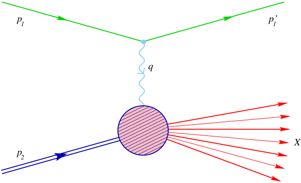
Figure 1.1: DIS: $p_{1}$ ($p_{1}^{\prime}$) represents the incoming (scattered) electron, $p_{2}$ the incoming proton, $q$ the exchanged virtual photon and $X$ the hadronic shower.

If the target proton has no spin polarization, the differential cross section can be parametrized by two Lorentz-invariant dimensionless structure functions according to App. A:

$${{\rm d}\sigma\over{\rm d}x\,{\rm d}Q^{2}}={2\pi\alpha^{2}\over xQ^{4}}\left\{[1+(1-y)^{2}]F_{2}(x,Q^{2})-y^{2}F_{L}(x,Q^{2})\right\}\;.$$ (1.4)

What can we say about the structure functions? Even if the final state is inclusive as far as the hadrons are concerned and we limit ourselves to sufficiently high transferred momenta $Q^{2}$, long distance effects are important in this kind of reaction. This is due to the fact that, in the initial state, a particular hadron (the proton) is recorded by measuring its momentum and therefore the process is not completely inclusive — it belongs to the second-type ones described in the previous section.

Suppose anyhow to undertake the perturbative calculation by assuming the proton composed of some quarks and gluons. At tree level, the calculation is lead back to the computation of the electron-quark Born cross section, but as soon as one consider 1-loop corrections, gluons set in and IR singularities (besides the UV ones) appear giving infinite cross sections.

Let’s stop for a while and try to understand what’s happening by looking at scattering in the center of mass (CM) frame. At high energy $\sqrt{s}\gg M$, the fast motion causes the proton to be Lorentz contracted in the direction of the collision and its internal interaction are time-dilated. Thus, the lifetime of any virtual partonic state is lengthened and the time it takes the electron to traverse the proton is shortened. When the latter is much shorter than the former, the proton will be in a single virtual state characterized by a definite number of partons during the entire time the electron takes to cross it. Since the partons in practice do not interact during this time, each one may be thought of as carrying a definite fraction $z$ of the proton’s momentum.

Furthermore, if we consider large momentum transfers $Q^{2}\gg M^{2}$, then the resolving power of the virtual photon is much smaller than the transverse size of the proton and the electron will be able to interact with only a single parton (provided the density of partons is not too high).

Under these conditions, the electron-parton amplitudes contribute incoherently, hence the scattering probability on the proton is given by the sum of the probabilities of scattering on the partons. The latter, in turn, can be thought to be inside the proton with certain probability distributions.

We have finally the following simple probabilistic interpretation: the electron-proton cross section is given by the sum over partons of the probabilities for electron-parton scattering, each of them weighted with the density distribution of that parton to be found inside the proton. This is the essence of the factorization theorem of collinear singularities [6] which, for the structure function, states

$$F_{i}^{(H)}(x,Q^{2})=\sum_{\text{\sf a}}\int_{x}^{1}{\rm d}z\;f^{(\text{\sf a}/H)}(z,Q^{2})\,\hat{F}_{i}^{(\text{\sf a})}\big{(}{x\over z},\alpha_{\mathrm{s}}(Q^{2})\big{)}\qquad(i=L,2)\;.$$ (1.5)

Here $f^{(\text{\sf a}/H)}(z,Q^{2}){\rm d}z$ is interpreted as the probabilityto find a parton of type a (= gluon, $u,\bar{u},d,\bar{d},s,\dots$) in a hadron of type $H$ carrying a fraction $z$ to $z+{\rm d}z$ of the hadron’s momentum ($p_{2}\equiv p$ in the following), while $\hat{F}_{i}^{(\text{\sf a})}(\hat{x}{},\alpha_{\mathrm{s}}(Q^{2}))$ is the partonic structure function (for the process $e\,\text{\sf a}\to e\,X$) with respect to the rescaled Bjorken variable

$$\hat{x}{}\,\raisebox{0.37pt}{:}={Q^{2}\over 2(zp)\cdot q}={x\over z}\;.$$

Note that the partonic distribution functions (PDF) have an explicit $Q^{2}$-dependence. In our intuitive picture this is due to the fact that additional partons — generated by virtual processes — can be resolved by increasing the value of $Q^{2}$.

1.5 The parton model

If we completely neglect interactions among partons, the parton content of the proton is fixed, i.e., independent of $Q^{2}$, since virtual processes are absent. Furthermore, the virtual photon can be absorbed only elastically by quarks, as depicted in Fig. 1.2.

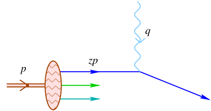
Figure 1.2: Elastic scattering of a quark by absorption of a virtual photon.

Since partons are considered massless objects in DIS, it holds

$$0=(zp+q)^{2}=(zp)^{2}+q^{2}+2z\,pq=z\,2pq-Q^{2}$$

or, equivalently

$$z={Q^{2}\over 2pq}=x\quad\Longrightarrow\quad\hat{x}{}={x\over z}=1\;.$$

This means that the Bjorken variable $x$ coincides with the momentum fraction of the active quark and that the partonic SF are proportional to $\delta(1-\hat{x}{})$. The explicit calculation of the partonic SF yields (omitting the hadron suffix $H$ hereafter)

$$\hat{F}_{2}^{(\text{\sf a})}(\hat{x}{},\alpha_{\mathrm{s}}=0) =e_{\text{\sf a}}^{2}\delta(1-\hat{x}{})\;,$$ (1.6a)

$$\hat{F}_{L}^{(\text{\sf a})}(\hat{x}{},\alpha_{\mathrm{s}}=0) =0\;,$$ (1.6b)

$e_{\text{\sf a}}$ being the EM charge (in unit of the electron charge) of type a partons.

The last equation (Callan-Gross relation) follows from the fact that a longitudinally polarized vector boson cannot be absorbed by a spin-$1/2$ quark (cfr. App. A). However the QCD corrections provide a non-zero coupling between longitudinal virtual photons and partons, so that $F_{L}={\mathcal{O}}(\alpha_{\mathrm{s}})$. The SF measurements show that $F_{L}\ll F_{2}$ (see Fig.1.3), confirming the spin $1/2$ property of quarks.

Figure 1.3: The longitudinal proton structure function $F_{L}$ data compared with the $F_{2}$ structure function fit (the black line).

Because of the $Q^{2}$-independence of both the PDF and the partonic SF, the SF depend only on the dimensionless variable $x$, as one would expect from a simple dimensional analysis. This is the so called scaling behavior [7]. The $Q^{2}$ dependence of $F_{2}$ for various values of $x$ is reported in Fig. 1.4. Approximate scaling is visible, especially around $x\simeq 0.2$. Anyway, scaling violations are also evident, and their origin is the subject of the next sections.

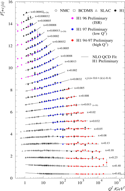
Figure 1.4: The proton structure function $F_{2}$ versus $Q^{2}$ for various values of $x$.

1.6 Scaling Violations

Historically, the first approach to next-to-leading order (NLO) corrections for DIS made use of the OPE. Even if a clear interpretation of the underlying physics will be available in the parton model picture, this formal approach will be useful in order (i) to classify the main contributions to scaling violations (by means of the so called twist index); (ii) to show explicitly the connection between anomalous dimensions of certain composite operators and evolution kernels for partonic distributions; (iii) to provide a first explanation of factorization of perturbative and non perturbative effects in strong interactions.

1.6.1 Operator product expansion (OPE)

Starting from the expression (A.4b) for the hadronic tensor

$$W_{\mu\nu}(p,q)={1\over 4\pi}\int{\rm d}^{4}z\;{\rm e}^{{\rm i}qz}\,{1\over 2}\sum_{\lambda=\text{spin}}\langle p,\lambda|[J_{\mu}(z),J_{\nu}(0)]|p,\lambda\rangle\;,$$ (1.7)

we note that the commutator of the EM currents vanishes for $z^{2}<0$. Furthermore, in the Bjorken limit $Q^{2}\to\infty$, $x$ fixed, the dominant domain of integration turns out to be $0\leqslant z^{2}\lesssim\text{const}/Q^{2}$, i.e., a thin sheet upon the forward light cone.

Notice that the product of two local operators at light-like distances is singular. Nevertheless, these singularities can be embodied in c-number functions by mean of the OPE [8] that near the light-cone takes the form

$$J(z)J(0)=\sum_{\omega=0}^{\infty}\sum_{\text{\sf j}}C_{\omega}^{(\text{\sf j})}(z^{2})\,z^{\mu_{1}}\cdots z^{\mu_{\omega}}\,O_{\mu_{1}\cdots\mu_{\omega}}^{(\text{\sf j})}\;,$$ (1.8)

where the c-number coefficient functions $C_{\omega}^{(\text{\sf j})}(z^{2})$ are eventually singular at $z^{2}=0$ and the composite operators $O_{\mu_{1}\cdots\mu_{\omega}}^{(\text{\sf j})}$ are well-defined objects, apart from the renormalization infinities. Anyhow, the singular behaviour in coordinate space is entirely carried by the coefficient functions.

In the Bjorken limit, all the masses can be neglected and the only dimensional variables in configuration space are the coordinates. A naïve dimensional analysis of Eq. (1.8) shows that, near the light-cone, the behaviour of the coefficient functions should be

$$C_{\omega}^{(\text{\sf j})}(z^{2})\simeq(z^{2})^{-3+\mbox{\small$\frac{1}{2}$}(d_{\omega}^{\text{\sf j}}-\omega)}\quad,\quad z^{2}\sim 0\;,$$ (1.9)

where $3=[J]$ and $d_{\omega}^{\text{\sf j}}=[O_{\mu_{1}\cdots\mu_{\omega}}^{(\text{\sf j})}]$ are the natural dimensions of the EM current and of the composite operators respectively.

In the non interacting theory the conformal invariance would require such a simple power-like behaviour. However in the interacting theory the above simple argument does not hold and in general logarithmic corrections to Eq. (1.9) develop after the renormalization procedure.

We see from Eq. (1.9) that, the smaller the twist value $d_{\omega}^{\text{\sf j}}-\omega$ is, the more singular $C_{\omega}^{(\text{\sf j})}$ will be, and then the dominant terms as $z^{2}\to 0$ ($Q^{2}\to\infty$) are controlled by the lowest twist operators, higher twists being suppressed by powers of $Q^{2}$.

There are two kinds of leading twist operators (twist $=2$) occurring in the OPE (1.8) for DIS:

$$O_{\mu_{1}\cdots\mu_{\omega}}^{(\text{\sf g})} =F_{\mu_{1}\lambda}{\cal D}_{\mu_{2}}\cdots{\cal D}_{\mu_{\omega-1}}F_{\mu_{\omega}}{}^{\lambda}\;,$$ (1.10a)

$$O_{\mu_{1}\cdots\mu_{\omega}}^{(\text{\sf f})} =\bar{\psi}{}^{(\text{\sf f})}\gamma_{\mu_{1}}{\mathcal{D}}_{\mu_{2}}\cdots{\mathcal{D}}_{\mu_{\omega}}\psi^{(\text{\sf f})}\quad,\quad(\text{\sf f}=1,\dots,N_{\!f})\;,$$ (1.10b)

$N_{\!f}$ being the number of (massless) flavours and ${\cal D}$ (${\mathcal{D}}$) the covariant derivative for gluons (quarks). The former are gluonic operators and the latter are quark operators.

It is to be stressed that the composite operators of Eqs. (1.10) appearing in the OPE do not depend on the hard probe (photon, weak boson, gluon, etc.) coupled to the hadronic tensor, and their hadronic matrix elements $A^{(\text{\sf j})}_{\omega}$ (cfr. Eq. (1.13)) describe only the partonic content of the initial particle $H$. In this sense, they are universal, i.e., the same for any hard reaction involving the same hadron $H$. However, the composite operators describe the long distance properties of the particles and therefore they cannot be calculable within perturbative QCD and their ignorance have to be compensated by some modellistic assumption or, better, by experimental measurements.

The coupling to the probe is accounted for by the coefficient functions, which are process dependent. They contains the informations of the short distance interactions between the exchanged boson and the constituents of the hadron as well as of high transfer momentum processes among partons. The following analysis will show how the former part of these short distance processes corresponds to the partonic SF and the latter one can be included in the PDF which acquire a (logarithmic) dependence on the virtuality $Q^{2}$ of the probe.

What is needed to derive the $Q^{2}$-dependence of the SF is

• to relate the objects of the OPE to the SF;

• to determine the $Q^{2}$-dependence of the coefficient functions (the composite operators being independent of $z$ and hence of $Q^{2}$).

The relations between OPE and SF have been derived in [9] and express the moments (i.e. the Mellin transforms) of the SF

$$F_{\omega}(Q^{2})\,\raisebox{0.37pt}{:}=\int_{0}^{1}{{\rm d}x\over x}\;x^{\omega}\,F(x,Q^{2})$$ (1.11)

in terms of the Fourier transforms of the coefficient functions

$$(Q^{2})^{\omega}\int{\rm d}^{4}z\;{\rm e}^{{\rm i}qz}\,z^{\mu_{1}}\cdots z^{\mu_{\omega}}\,C_{\omega}^{(\text{\sf j})}(z^{2})=\raisebox{0.37pt}{:}\hskip 3.0ptq^{\mu_{1}}\cdots q^{\mu_{\omega}}\,\widetilde{C}_{\omega-1}^{(\text{\sf j})}(Q^{2})$$ (1.12)

and of the matrix elements

$${1\over 2}\sum_{\lambda}\langle p,\lambda|O_{\mu_{1}\cdots\mu_{\omega}}^{(\text{\sf j})}|p,\lambda\rangle=A_{\omega-1}^{(\text{\sf j})}\,p_{\mu_{1}}\cdots p_{\mu_{\omega}}+\text{terms containing }g_{\mu_{i}\mu_{k}}$$ (1.13)

in the famous moment sum rules

$$F_{\omega}(Q^{2})=\sum_{\text{\sf j}}A_{\omega}^{(\text{\sf j})}\,C_{\omega}^{(\text{\sf j})}(Q^{2})\;.$$ (1.14)

The determination of the coefficient function dependence on $Q^{2}$ can be done by using the RG technique[10]. The renormalization procedure, necessary to handle the infinities stemming from the perturbative expansion, requires the introduction of a mass parameter $\mu$ (the renormalization scale) not present in the original lagrangian. As $\mu$ is an artificial parameter, the physical quantities — in our case the SF — do not depend on it. This constraint determine the $\mu$-dependence of the coefficient functions, of the composite operators and of the coupling as well.

In addition, the dimensionless coefficient functions and the coupling can depend on the massive parameter $Q^{2}$ and $\mu$ only through the ratio $Q^{2}/\mu^{2}$. Therefore, their $Q^{2}$-dependence is completely calculable within perturbative QCD and, by means of Eq. (1.14), we obtain the $Q^{2}$ dependence of the SF.

In particular, the RG equation for the coefficient function is

$$\left[\left(\mu{\partial\over\partial\mu}+2\beta(\alpha_{\mathrm{s}}){\partial\over\partial\alpha_{\mathrm{s}}}\right)\delta^{\text{\sf j}\text{\sf k}}+({\boldsymbol{\gamma}}_{\omega})^{\text{\sf j}\text{\sf k}}\right]\widetilde{C}_{\omega}^{(\text{\sf k})}\big{(}Q^{2}/\mu^{2},\alpha_{\mathrm{s}}(\mu^{2})\big{)}=0\qquad\forall\;\text{\sf j}\;,$$ (1.15)

where the indices j and k label the different types of operators in Eqs. (1.10) and ${\boldsymbol{\gamma}}_{\omega}$ is (the opposite of) their anomalous dimension matrix:

$${\boldsymbol{\gamma}}_{\omega} \,\raisebox{0.37pt}{:}=-\boldsymbol{Z}_{\omega}^{-1}\left(\mu{\partial\over\partial\mu}\boldsymbol{Z}_{\omega}\right)\quad,\quad O_{\mu_{1}\cdots\mu_{\omega}}^{(\text{\sf j}),\text{bare}}=\left[\boldsymbol{Z}_{\omega}\right]^{\text{\sf j}\text{\sf k}}O_{\mu_{1}\cdots\mu_{\omega}}^{(\text{\sf k}),\text{renormalized}}\;,$$ (1.16)

$${\boldsymbol{\gamma}}_{\omega} =\raisebox{0.37pt}{:}\hskip 3.0pt\alpha_{\mathrm{s}}\,\overset{\mbox{\text{\tiny(1)}}}{{\boldsymbol{\gamma}}}{}_{\omega}+\alpha_{\mathrm{s}}^{2}\,\overset{\mbox{{\tiny(2)}}}{{\boldsymbol{\gamma}}}{}_{\omega}+\cdots\;.$$ (1.17)

The solution of Eq. (1.15) is found by introducing the running coupling function of Eq. (1.1) and can be written as a path-ordered exponential

$$\widetilde{C}_{\omega}^{(\text{\sf j})}(Q^{2}/\mu^{2},\alpha_{\mathrm{s}}(\mu^{2}))=\mathbb{T}\exp\left\{\int_{\alpha_{\mathrm{s}}(\mu^{2})}^{\alpha_{\mathrm{s}}(Q^{2})}{{\boldsymbol{\gamma}}_{\omega}(\alpha)\over\beta(\alpha)}\;{\rm d}\alpha\right\}^{\text{\sf j}\text{\sf k}}\widetilde{C}_{\omega}^{(\text{\sf k})}\big{(}1,\alpha_{\mathrm{s}}(Q^{2})\big{)}\;,$$ (1.18)

showing that the coefficient functions depend on $Q^{2}$ only through the running coupling $\alpha_{\mathrm{s}}(Q^{2})$.

1.6.2 The “running” parton distribution functions

The formal results (1.14) and (1.18) can be given a simple and elegant interpretation in terms of PDF which depend upon $Q^{2}$: we can write at LO in $\ln Q^{2}$

$$F_{i,\omega}(Q^{2})=\sum_{\text{\sf j},\text{\sf k}}A_{\omega}^{(\text{\sf j})}\left[{\alpha_{\mathrm{s}}(\mu^{2})\over\alpha_{\mathrm{s}}(Q^{2})}\right]^{\overset{\mbox{\text{\tiny(1)}}}{{\boldsymbol{\gamma}}}\!{}_{\omega}/b_{0}}_{\;\text{\sf j}\text{\sf k}}\widetilde{C}_{i,\omega}^{(\text{\sf k})}(1,0)\;\times\;\left[1+{\mathcal{O}}(1/\ln Q^{2})\right]\;.$$ (1.19)

First of all, switch off for a minute the strong interaction, so that $\alpha_{\mathrm{s}}(Q^{2})=\alpha_{\mathrm{s}}(\mu^{2})=0$ and

$$F_{i,\omega}(Q^{2})=F_{i,\omega}=\sum_{\text{\sf j}}A_{\omega}^{(\text{\sf j})}\,\widetilde{C}_{i,\omega}^{(\text{\sf j})}(1,0)\;.$$ (1.20)

If we take the Mellin transform of Eq. (1.5) by defining

$$\hat{F}_{i,\omega}^{(\text{\sf a})}\big{(}\alpha_{\mathrm{s}}(Q^{2})\big{)} \,\raisebox{0.37pt}{:}=\int_{0}^{1}{{\rm d}x\over x}\;x^{\omega}\,\hat{F}_{i}^{(\text{\sf a})}\big{(}x,\alpha_{\mathrm{s}}(Q^{2})\big{)}\;,$$ (1.21)

$$f_{\omega}^{(\text{\sf a})}(Q^{2}) \,\raisebox{0.37pt}{:}=\int_{0}^{1}{\rm d}x\;x^{\omega}\,f^{(\text{\sf a})}(x,Q^{2})\;,$$ (1.22)

the moments of the SF turns out to be simply

$$F_{i,\omega}=\sum_{\text{\sf a}}f_{\omega}^{(\text{\sf a})}(Q^{2})\,\hat{F}_{i,\omega}^{(\text{\sf a})}(0)\;.$$ (1.23)

In this situation it is natural to identify the short distance and long distance factors as

$$\widetilde{C}_{i,\omega}^{(\text{\sf a})}(1,0) \longleftrightarrow\hat{F}_{i,\omega}^{(\text{\sf a})}(0)\;,$$ (1.24)

$$A_{\omega}^{(\text{\sf a})} \longleftrightarrow f_{\omega}^{(\text{\sf a})}(Q^{2})=f_{\omega}^{(\text{\sf a})}\;.$$ (1.25)

Equivalently, one can obtain the parton model picture (1.5) by performing the inverse Mellin transform of Eq. (1.20) by suitably identifying PDF and partonic SF.

We can go further by applying the same reasoning in the interacting case, in which we use again Eq. (1.24) — because at LO the partonic SF are $Q^{2}$-independent — together with the new identification

$$\sum_{\text{\sf a}}A_{\omega}^{(\text{\sf a})}\left[{\alpha_{\mathrm{s}}(\mu^{2})\over\alpha_{\mathrm{s}}(Q^{2})}\right]^{\overset{\mbox{\text{\tiny(1)}}}{{\boldsymbol{\gamma}}}\!{}_{\omega}/b_{0}}_{\;\text{\sf a}\text{\sf b}}\longleftrightarrow f_{\omega}^{(\text{\sf b})}(Q^{2})\;.$$ (1.26)

in such a way that the $Q^{2}$-dependence is incorporated in the PDF.

At this point we differentiate the above relation with respect to $\ln Q^{2}$ and, taking into account Eqs. (1.1) and (1.3), we end up with the evolution equation for the moments of the PDF

$${{\rm d}\over{\rm d}\ln Q^{2}}f_{\omega}^{(\text{\sf a})}(Q^{2})=\sum_{\text{\sf b}}\alpha_{\mathrm{s}}(Q^{2})[\overset{\mbox{\text{\tiny(1)}}}{{\boldsymbol{\gamma}}}\!{}_{\omega}]^{\text{\sf a}\text{\sf b}}f_{\omega}^{(\text{\sf b})}(Q^{2})\quad,\quad\text{\sf a}=\text{\sf f},\bar{\text{\sf f}},\text{\sf g}\;.$$ (1.27)

This set of $2N_{\!f}+1$ coupled differential equations can be diagonalized by analysing the properties of the PDF under flavour symmetry — which is an exact symmetry if quark masses are neglected.

Clearly, the gluon density $f^{(\text{\sf g})}$ is invariant under flavour transformations, as well as the “modulus” of the quark vector

$$f^{(\Sigma)}(x,Q^{2})\,\raisebox{0.37pt}{:}=\sum_{\text{\sf f}}f^{(\text{\sf f})}(x,Q^{2})+f^{(\bar{\text{\sf f}})}(x,Q^{2})$$ (1.28)

called quark singlet density.

The non-singlet (NS) components of the quark densities, transforming according to the adjoint representation of $SU(N_{\!f})$, are constructed by subtracting from the various fermionic PDF the common singlet component:

$$f^{(\text{NS},\text{\sf f})}(x,Q^{2})\,\raisebox{0.37pt}{:}=f^{(\text{\sf f})}(x,Q^{2})-{1\over 2N_{\!f}}f^{(\Sigma)}(x,Q^{2})\;.$$ (1.29)

Since the NS quark densities carries different quantum numbers (flavours) they don’t mix and renormalize independently. Furthermore, the flavour group commutes with the colour group, so all NS densities evolve with the same quark-to-quark anomalous dimension $\gamma^{\text{\sf q}\text{\sf q}}$

$${{\rm d}\over{\rm d}\ln Q^{2}}f_{\omega}^{(\text{NS},\text{\sf f})}(Q^{2})=\alpha_{\mathrm{s}}(Q^{2})\,\overset{\mbox{\text{\tiny(1)}}}{\gamma}{}^{\text{\sf q}\text{\sf q}}_{\omega}\,f_{\omega}^{(\text{NS},\text{\sf f})}(Q^{2})\;.$$ (1.30)

Only quark singlet and gluon operators mix in the renormalization and require a $2\times 2$ anomalous dimension matrix such that

$${{\rm d}\over{\rm d}\ln Q^{2}}\begin{pmatrix}f_{\omega}^{(\Sigma)}(Q^{2})\\ f_{\omega}^{(\text{\sf g})}(Q^{2})\end{pmatrix}=\alpha_{\mathrm{s}}(Q^{2})\begin{pmatrix}\overset{\mbox{\text{\tiny(1)}}}{\gamma}{}^{\text{\sf q}\text{\sf q}}_{\omega}&2N_{\!f}\,\overset{\mbox{{\tiny(1)}}}{\gamma}{}^{\text{\sf q}\text{\sf g}}_{\omega}\\ \overset{\mbox{{\tiny(1)}}}{\gamma}{}^{\text{\sf g}\text{\sf q}}_{\omega}&\overset{\mbox{{\tiny(1)}}}{\gamma}{}^{\text{\sf g}\text{\sf g}}_{\omega}\end{pmatrix}\begin{pmatrix}f_{\omega}^{(\Sigma)}(Q^{2})\\ f_{\omega}^{(\text{\sf g})}(Q^{2})\end{pmatrix}\;.$$ (1.31)

Using Eq. (1.22) and the splitting functions implicitly defined by

$$\gamma_{\omega}^{\text{\sf a}\text{\sf b}}=\raisebox{0.37pt}{:}\hskip 3.0pt{\alpha_{\mathrm{s}}(Q^{2})\over 2\pi}\int_{0}^{1}{\rm d}z\;z^{\omega}\,P^{\text{\sf a}\text{\sf b}}(z)\;,$$ (1.32)

we can invert Eqs. (1.30) and (1.31) in $x$ space and reproduce the famous Dokshitzer-Gribov-Lipatov-Altarelli-Parisi (DGLAP) equations [11]

$${{\rm d}\over{\rm d}\ln Q^{2}}f^{(\text{NS},\text{\sf f})}(x,Q^{2}) ={\alpha_{\mathrm{s}}(Q^{2})\over 2\pi}\int_{x}^{1}{\rm d}z\;\overset{\mbox{{\tiny(1)}}}{P}{}^{\text{\sf q}\text{\sf q}}\big{(}{x\over z}\big{)}\,f^{(\text{NS},\text{\sf f})}(z,Q^{2})\;,$$ (1.33a)

$${{\rm d}\over{\rm d}\ln Q^{2}}f^{(\Sigma)}(x,Q^{2}) ={\alpha_{\mathrm{s}}(Q^{2})\over 2\pi}\int_{x}^{1}{\rm d}z\;\overset{\mbox{{\tiny(1)}}}{P}{}^{\text{\sf q}\text{\sf q}}\big{(}{x\over z}\big{)}\,f^{(\Sigma)}(z,Q^{2})+2N_{\!f}\overset{\mbox{{\tiny(1)}}}{P}{}^{\text{\sf q}\text{\sf g}}\big{(}{x\over z}\big{)}\,f^{(\text{\sf g})}(z,Q^{2})\;,$$ (1.33b)

$${{\rm d}\over{\rm d}\ln Q^{2}}f^{(\text{\sf g})}(x,Q^{2}) ={\alpha_{\mathrm{s}}(Q^{2})\over 2\pi}\int_{x}^{1}{\rm d}z\;\overset{\mbox{{\tiny(1)}}}{P}{}^{\text{\sf g}\text{\sf q}}\big{(}{x\over z}\big{)}\,f^{(\Sigma)}(z,Q^{2})+\overset{\mbox{{\tiny(1)}}}{P}{}^{\text{\sf g}\text{\sf g}}\big{(}{x\over z}\big{)}\,f^{(\text{\sf g})}(z,Q^{2})\;.$$ (1.33c)

It is also possible to diagonalize the anomalous dimension matrix of the singlet sector by determining the eigenvalues

$$\gamma_{\omega}^{\pm}={1\over 2}\left(\gamma^{\text{\sf q}\text{\sf q}}_{\omega}+\gamma^{\text{\sf g}\text{\sf g}}_{\omega}\pm\sqrt{(\gamma^{\text{\sf q}\text{\sf q}}_{\omega}-\gamma^{\text{\sf g}\text{\sf g}}_{\omega})^{2}+8N_{\!f}\gamma^{\text{\sf q}\text{\sf g}}_{\omega}\gamma^{\text{\sf g}\text{\sf q}}_{\omega}}\right)$$ (1.34)

and the eigenvectors

$$f_{\omega}^{(\pm)}=f_{\omega}^{(\text{\sf g})}+{\gamma_{\omega}^{\pm}-\gamma^{\text{\sf g}\text{\sf g}}_{\omega}\over 2N_{\!f}\gamma^{\text{\sf q}\text{\sf g}}_{\omega}}f_{\omega}^{(\Sigma)}(Q^{2})\;,$$ (1.35)

so that

$${{\rm d}\over{\rm d}\ln Q^{2}}f_{\omega}^{(\pm)}(Q^{2})=\alpha_{\mathrm{s}}(Q^{2})\gamma_{\omega}^{\pm}f_{\omega}^{(\pm)}(Q^{2})\;.$$ (1.36)

b $\leftarrow$ a	$\overset{\mbox{{\tiny(1)}}}{P}{}^{\text{\sf b}\text{\sf a}}(z)$	$2\pi\overset{\mbox{{\tiny(1)}}}{\gamma}{}_{\omega}^{\text{\sf b}\text{\sf a}}$
q   q	$\displaystyle{C_{F}\left(\frac{1+z^{2}}{1-z}\right)_{\!\!{}_{+}}}$	$\displaystyle{C_{F}\left[{3\over 2}+{1\over(\omega+1)(\omega+2)}+2\psi(1)-2\psi(\omega+2)\right]}$
g   q	$\displaystyle{C_{F}\left[\frac{1+(1-z)^{2}}{z}\right]}$	$\displaystyle{C_{F}\,{\omega^{2}+3\omega+4\over\omega(\omega+1)(\omega+2)}}$
q   g	$\displaystyle{T_{R}\left[z^{2}+(1-z)^{2}\right]}$	$\displaystyle{T_{R}\,{\omega^{2}+3\omega+4\over(\omega+1)(\omega+2)(\omega+3)}}$
g   g	$\displaystyle{2C_{A}\left[\frac{1-z}{z}+\frac{z}{(1-z)_{{}_{+}}}+z(1-z)\right]+\delta(1-z)}$	$\displaystyle{\left[{11C_{A}\over 6}-{N_{\!f}\over 3N_{c}^{2}}\right]}\;$
		$\displaystyle{2C_{A}\left[{11\over 12}+{1\over\omega(\omega+1)}+{1\over(\omega+2)(\omega+3)}+\psi(1)-\psi(\omega+2)\right]-{N_{\!f}\over 3N_{c}^{2}}}$
		$\displaystyle{C_{A}=N_{c}\;,\;C_{F}={N_{c}^{2}-1\over 2N_{c}}\;,\;T_{R}={1\over 2}\;,\quad\int_{x}^{1}f(z)g_{+}(z){\rm d}z:=\int_{x}^{1}[f(z)-f(1)]g(z)\,{\rm d}z-f(1)\int_{0}^{x}g(z)\,{\rm d}z}$

Table 1.1: The 1-loop partonic splitting functions and anomalous dimensions.

To summarize the results of the previous sections, we have shown that a certain number of observables of hard inclusive processes can be expressed as a convolution of process dependent, perturbative calculable, partonic cross sections and universal, non perturbative, partonic distribution functions inside hadrons whose dependence on the virtuality $Q^{2}$ of the hard probe is however computable within the framework of perturbative QCD. This means that we are not in such a position to say what the value of $F_{2}(x=0.1,Q^{2}=10\;\text{GeV}^{2})$ is, but if we measure with enough accuracy the $x$-dependence of a sufficient number of structure functions at a certain value of $Q^{2}\gg\Lambda^{2}$, we can predict their behaviour at higher $Q^{2}$ values. Furthermore, the consequent knowledge of the PDF allows us to predict absolute values of cross sections for completely different hadronic processes. This is very important as a test of the theory as well as experimentally, in order to check normalization on the cross sections, to estimate the occurrence of yet unobserved phenomena, etc..

1.7 The improved parton model

In the following, we shall show an alternative approach for dealing with scaling violations in DIS. This method presents several advantages with respect to the OPE shown before.

On one hand, there are very few reactions where one can justify the use of the OPE. It is therefore of great importance to rephrase the physics in the language of a very general QCD-improved parton model by which we can study a larger variety of phenomena.

On the other hand the improved parton model gives the LO results in a much more intuitive and economical way and permits, with reasonable efforts, to perform NLO calculations (e.g., the NLO anomalous dimensions).

In addition, — and this is the main reason of this lengthy discussion — the partonic framework clarifies the connection between general field-theoretical predictions, such as factorization and OPE, and the resummation of certain classes of Feynman diagrams. A very similar formalism will be very useful when dealing with high energy reactions, where Regge theory, BFKL dynamics, high energy factorization and RG constraints meet in describing semi-hard processes. Also in this case the partonic picture turns out to be of fundamental importance to extend the calculation to next-to-leading level and to take into account a whole series of sub-leading contributions to all orders, which is the central purpose of the present thesis.

1.7.1 Next-to-leading order parton model

Having convinced ourselves of the factorization properties splitting strong coupling from perturbative physics, we are going to attack the problem from another point of view. We assume the hadron undergoing DIS to be composed of several partons $\text{\sf a}=\text{\sf f},\bar{\text{\sf f}},\text{\sf g}$ with distribution densities $f^{(\text{\sf a})}(\xi)$, $\xi$ being the longitudinal momentum fraction of the parton. We assume also that parton-photon and parton-parton interactions can be treated perturbatively. The validity conditions and consequences of these hypotheses are what we wish to present.

Since among partons only quarks carry EM charge, the partonic interaction at Born level is represented uniquely by the diagram in Fig. 1.5, where $\hat{p}{}=\xi p$ is the incoming quark momentum. The ensuing partonic tensor reads

$$\hat{W}{}_{\mu\nu}^{(\text{\sf a},0)}(\hat{p}{},q) =e_{\text{\sf a}}^{2}\delta(1-\hat{x}{})\Gamma_{\mu\nu}(\hat{p}{},q)$$ (1.37a)

$$\Gamma_{\mu\nu}(\hat{p}{},q) =-{1\over 2}\left(g_{\mu\nu}-{q_{\mu}q_{\nu}\over q^{2}}\right)+{1\over\hat{p}{}q}\left(\hat{p}{}_{\mu}-{\hat{p}{}q\over q^{2}}q_{\mu}\right)\left(\hat{p}{}_{\nu}-{\hat{p}{}q\over q^{2}}q_{\nu}\right)\;,$$ (1.37b)

whose longitudinal and transverse projections give the partonic SF of Eqs. (1.6).

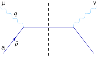
Figure 1.5: The diagram representing the partonic tensor $\hat{W}{}_{\mu\nu}^{(\text{\sf a},0)}$ at Born level. a labels the incoming quark flavour an $\hat{p}{}$ its momentum.

At NLO, we should take into account all the insertions of a gluonic line in Fig. 1.5 such as Fig. 1.6a and also gluon-photon coupling via a quark-loop like in Fig. 1.6b.

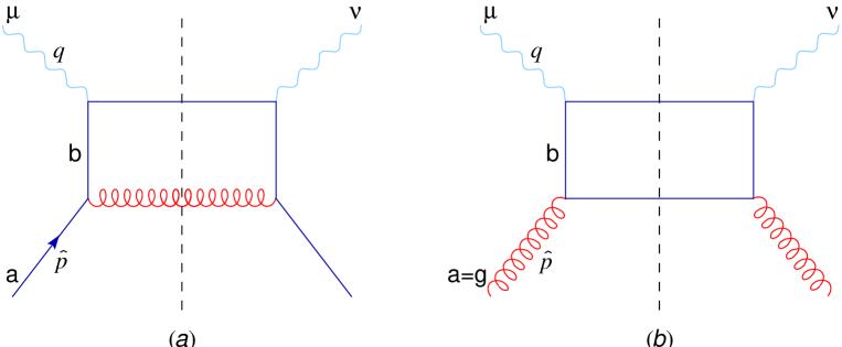
Figure 1.6: Examples of 1-loop couplings: quark-photon (a) and gluon-photon (b).

Let’s start computing the real emission diagram of Fig. 1.6a in the kinematic regime $Q^{2}\gg M^{2}$ and $x,1-x$ not too small, where we expect scaling violations. In this regime, quarks can be considered massless, but in so doing the integration over the internal momenta $k$ diverges when the transverse component ${\boldsymbol{k}}$ vanishes, i.e., when the internal quark and the outgoing gluon are emitted collinearly (collinear singularity). In our notations, all boldface transverse vectors have to be considered $D-2$ dimensional vectors with euclidean components, such that ${\boldsymbol{k}}^{2}>0$.

By means of a suitable regularization, by introducing for instance a (small) cutoff $\lambda$, we end up with a finite result which has the interesting feature of containing a term proportional to $\ln Q^{2}/\lambda^{2}$. The same behaviour is shown by the diagram in Fig. 1.6b.

This logarithmic factor comes from the ${\boldsymbol{k}}$-integration

$$\int_{|{\boldsymbol{k}}|_{\text{min}}}^{|{\boldsymbol{k}}|_{\text{max}}}{{\rm d}^{2}{\boldsymbol{k}}\over{\boldsymbol{k}}^{2}}\propto\ln{Q^{2}\over\lambda^{2}}\quad;\quad{\boldsymbol{k}}_{\text{min}}^{2}=\lambda^{2}\quad;\quad{\boldsymbol{k}}_{\text{max}}^{2}=Q^{2}{1-\hat{x}{}\over 4\hat{x}{}}=\text{(small const)}Q^{2}\;.$$ (1.38)

It is crucial to note that to the IR logarithmic collinear singularity corresponds a $\ln Q^{2}$ term arising from the hard ${\boldsymbol{k}}$ component of the emitted quark. This is obvious from a simple dimensional analysis, $Q^{2}$ being the only dimensional scale which can accompany the cutoff $\lambda^{2}$ in the logarithm. Conversely, to each $\ln Q^{2}$ is in fact associated a collinear logarithmic singularity so that one can investigate the structure of the latter for determining the former. Here resides the intimate connection between collinear singularities and scaling violations.

The presence of a large $\ln Q^{2}$ at ${\mathcal{O}}(\alpha_{\mathrm{s}})$ should warn us as far as the convergence of the perturbative series is concerned. In fact, taking for $\alpha_{\mathrm{s}}$ its running value $\alpha_{\mathrm{s}}(Q^{2})\sim 1/\ln Q^{2}$, the NLO correction $\sim\alpha_{\mathrm{s}}(Q^{2})\ln Q^{2}\sim 1$ may be large even for small coupling. This is exactly what happens at higher orders, where in the ${\mathcal{O}}(\alpha_{\mathrm{s}}^{n})$ contribution we find terms proportional to $\alpha_{\mathrm{s}}^{n}(Q^{2})\ln^{n}(Q^{2})\sim 1$. Therefore the relative importance of all the sub-leading corrections may be the same, and in order to provide quantitative estimates, all of them ought to be taken into account through a suitable resummation procedure.

The first step of a resummation procedure consists in rearranging the perturbative series according to a new hierarchy, the first term of which is formed by the “largest” contributions $\sim[\alpha_{\mathrm{s}}\ln Q^{2}]^{n}:n=0,1,\cdots$ (leading logarithmic (LL) approximation), the second one containing one power of $\alpha_{\mathrm{s}}$ more than the first one, i.e., $\sim\alpha_{\mathrm{s}}[\alpha_{\mathrm{s}}\ln Q^{2}]^{n}$ (next-to-leading logarithmic (NLL) approximation), the third one (NNLL) $\sim\alpha_{\mathrm{s}}^{2}[\alpha_{\mathrm{s}}\ln Q^{2}]^{n}$ and so on.

The second step requires the determination of all the LL terms in the perturbative series by identifying an iterating common structure — typically an integral kernel — representing the building block of the corresponding Feynman diagrams.

In the third step one expresses the unknown resummed object by means of an equation — typically an integro-differential one — whose basic ingredient is the iterating structure previously mentioned.

Finally, one has to solve the resumming equation as best as he or she (or the computer) can, to check its consistency, to try to fit the data and, possibly, restarting from the beginning in the next logarithmic approximation.

In this section we are dealing with the real emission, 1-loop correction to SF at leading $\ln Q^{2}$ level. For both 1.6a and b processes, the logarithmic term stems from the integration over the internal quark transverse momentum (Eq. (1.38)). The link with the collinear singularity tells us that the coefficient of $\ln Q^{2}$ is given by the residue of the $1/{\boldsymbol{k}}^{2}$ pole.

What about other real emission diagrams? Following the resummation program, we have to identify the diagrams furnishing the LL terms we are looking for. It turns out that, adopting axial gauges, i.e., including only physical transverse polarizations in the gluon propagators, only the diagrams 1.6a and b contributes in the LL approximation.

It is convenient to introduce the Sudakov parametrization

$$k=z\hat{p}{}+\bar{z}q^{\prime}+{\boldsymbol{k}}\quad,\quad q^{\prime}\,\raisebox{0.37pt}{:}=q+\hat{x}{}\hat{p}{}\quad,\quad\hat{x}{}\,\raisebox{0.37pt}{:}={-q^{2}\over 2\hat{p}{}\cdot q}\;,$$ (1.39)

which are nothing but the components of $k$ with respect to the light-like vectors $\hat{p}{}$ and $q^{\prime}$ plus the transverse component. In our notations, $k^{2}=2z\bar{z}\,\hat{p}{}\cdot q^{\prime}-{\boldsymbol{k}}^{2}$ and ${\boldsymbol{k}}^{2}>0$. For vanishingly small values of ${\boldsymbol{k}}$, the mass-shell constraints of the outgoing partons force $\bar{z}\simeq 0$ and $z\simeq\hat{x}{}$ so that the only relevant variable (upon which the residue depends) is the momentum fraction $\hat{x}{}$ of $k$ with respect to $\hat{p}{}$.

The residue of the collinear singularities of Figs. 1.6.a and b turns out to be respectively

$${\alpha_{\mathrm{s}}\over 2\pi}P^{\text{\sf b}\text{\sf f}}(z) ={\alpha_{\mathrm{s}}\over 2\pi}\delta^{\text{\sf b}\text{\sf f}}P^{\text{\sf q}\text{\sf q}}(z)\;,$$ (1.40a)

$${\alpha_{\mathrm{s}}\over 2\pi}P^{\text{\sf b}\text{\sf g}}(z) ={\alpha_{\mathrm{s}}\over 2\pi}P^{\text{\sf q}\text{\sf g}}(z)\;,$$ (1.40b)

where q denotes a generic quark or antiquark and the quark-to-quark and gluon-to-quark splitting functions read

$$P^{\text{\sf q}\text{\sf q}}(z) =C_{F}{1+z^{2}\over 1-z}\;,$$ (1.41)

$$P^{\text{\sf q}\text{\sf g}}(z) =T_{R}[z^{2}+(1-z)^{2}]\;.$$ (1.42)

The partonic tensor $\hat{W}{}_{\mu\nu}^{(\text{\sf a})}$ at first order in $\alpha_{\mathrm{s}}$ assumes then the form ($\hat{p}{}=\xi p$)

$$\left[\hat{W}{}_{\mu\nu}^{(0)}+\alpha_{\mathrm{s}}\hat{W}{}_{\mu\nu}^{(1)}\right]^{(\text{\sf a})}(\hat{p}{},q) =e_{\text{\sf a}}^{2}\delta(1-\hat{x}{})\Gamma_{\mu\nu}(\hat{p}{},q)+\sum_{\text{\sf b}}e_{\text{\sf b}}^{2}{\alpha_{\mathrm{s}}\over 2\pi}\ln{Q^{2}\over\lambda^{2}}\,P^{\text{\sf b}\text{\sf a}}(\hat{x}{})\Gamma_{\mu\nu}(\hat{x}{}\hat{p}{},q)$$

$$=\sum_{\text{\sf b}}\int_{0}^{\xi}{{\rm d}u\over u}\;\hat{W}{}_{\mu\nu}^{(\text{\sf b},0)}(up,q)\left[\delta^{\text{\sf b}\text{\sf a}}\delta\big{(}1-{u\over\xi}\big{)}+{\alpha_{\mathrm{s}}\over 2\pi}\ln{Q^{2}\over\lambda^{2}}\,P^{\text{\sf b}\text{\sf a}}\big{(}{u\over\xi}\big{)}\right]\;.$$ (1.43)

It is tempting to suppose that the hadronic tensor $W_{\mu\nu}(p,q)$ could be obtained by summing up the partonic ones $\hat{W}{}_{\mu\nu}^{(\text{\sf a})}(\xi p,q)$ weighted with the parton densities $f^{(\text{\sf a})}(\xi)$. Including the $1/\xi$ flux factor for compensate the fractional momentum of the incoming parton with respect to the proton, we try writing

$$W_{\mu\nu}(p,q) =\sum_{\text{\sf a}}\int_{x}^{1}{{\rm d}\xi\over\xi}\;\hat{W}{}_{\mu\nu}^{(\text{\sf a})}(\xi p,q)f^{(\text{\sf a})}(\xi)$$ (1.44)

$$=\sum_{\text{\sf b}}\int_{x}^{1}{{\rm d}u\over u}\;\hat{W}{}_{\mu\nu}^{(\text{\sf b},0)}(up,q)\left[\left(\boldsymbol{1}+{\alpha_{\mathrm{s}}\over 2\pi}\ln{Q^{2}\over\lambda^{2}}\,P\right)\otimes f\right]^{(\text{\sf a})}\!\!(u)\;,$$ (1.45)

where in the last equality we have changed the order of integration $\xi\leftrightarrow u$ and introduced the shorthand notation for convolutions

$$\big{[}f\otimes g\big{]}(u)\,\raisebox{0.37pt}{:}=\int_{u}^{1}{{\rm d}\xi\over\xi}\;f(\xi)g\big{(}{u\over\xi}\big{)}\;,$$ (1.46)

in which a sum over partonic indices is eventually understood.

A couple of remarks are in order:

• we are still in presence of the IR singularity $\lambda\to 0$ which prevents us from interpreting Eq. (1.45) as a reliable expression for $W_{\mu\nu}$;

• we have used perturbative theory in the (strong coupling) IR region $k^{2}\simeq-{\boldsymbol{k}}^{2}\to 0$ without being allowed to. $\alpha_{\mathrm{s}}$ is not yet running, but can we expect to have obtained the right answer?

The way to handle and to eliminate these drawbacks is easily explained. Let $\mu_{F}\gg\Lambda$ be a sufficiently hard mass scale, called factorization scale. We believe perturbation theory for $|k^{2}|\simeq{\boldsymbol{k}}^{2}\geqslant\mu_{F}^{2}$, while we cannot say anything for ${\boldsymbol{k}}^{2}<\mu_{F}^{2}$. However, the bare parton densities are completely unknown, so if we insert the non perturbative contribution $\lambda^{2}\leqslant{\boldsymbol{k}}^{2}<\mu_{F}^{2}$ in $f$ redefining the partonic distributions, we don’t introduce any new uncertainty in Eq. (1.45). Furthermore, in so doing the new partonic distributions absorb the collinear singularities which do not affect $W_{\mu\nu}$ anymore. In practice, we write, at ${\mathcal{O}}(\alpha_{\mathrm{s}})$ accuracy,

$$\left(\boldsymbol{1}+{\alpha_{\mathrm{s}}\over 2\pi}\ln{Q^{2}\over\lambda^{2}}\,P\right)\otimes f=\left(\boldsymbol{1}+{\alpha_{\mathrm{s}}\over 2\pi}\ln{Q^{2}\over\mu_{F}^{2}}\,P\right)\otimes\left(\boldsymbol{1}+{\alpha_{\mathrm{s}}\over 2\pi}\ln{\mu_{F}^{2}\over\lambda^{2}}\,P\right)$$ (1.47)

and define

$$f^{(\text{\sf a})}(\xi,\mu_{F}^{2})\,\raisebox{0.37pt}{:}=\left[\left(\boldsymbol{1}+{\alpha_{\mathrm{s}}\over 2\pi}\ln{\mu_{F}^{2}\over\lambda^{2}}\,P\right)\otimes f\right]^{(\text{\sf a})}\!\!(\xi)\;,$$ (1.48)

to be considered as an input parameter.

By writing the $W$ tensors in terms of (partonic) structure functions, Eq. (1.45) yields

$$F_{i}(x,Q^{2})=\sum_{\text{\sf a}}\int_{x}^{1}{\rm d}z\;\hat{F}{}_{i}^{(\text{\sf a})}\big{(}{x\over z}\big{)}\left[\left(\boldsymbol{1}+{\alpha_{\mathrm{s}}\over 2\pi}\ln{Q^{2}\over\mu_{F}^{2}}\,P\right)\otimes f_{\mu_{F}^{2}}\right]^{(\text{\sf a})}\!\!(z)\qquad(i=2,L)\;.$$ (1.49)

Obviously, the RHS of the above equation cannot depend on the artificial parameter $\mu_{F}$.

It is natural to define the $Q^{2}$-dependent PDF as

$$f^{(\text{\sf a})}(z,Q^{2})\,\raisebox{0.37pt}{:}=f^{(\text{\sf a})}(z,\mu_{F}^{2})+{\alpha_{\mathrm{s}}\over 2\pi}\ln{Q^{2}\over\mu_{F}^{2}}\sum_{\text{\sf b}}\int_{z}^{1}{{\rm d}\xi\over\xi}\;P^{\text{\sf a}\text{\sf b}}\big{(}{z\over\xi}\big{)}f^{(\text{\sf b})}(\xi,\mu_{F}^{2})$$ (1.50)

ending up with the desired factorization formula

$$F_{i}(x,Q^{2})=\sum_{\text{\sf a}}\int_{x}^{1}{\rm d}z\;f^{(\text{\sf a})}(z,Q^{2})\,\hat{F}{}_{i}^{(\text{\sf a})}\big{(}{x\over z}\big{)}\;.$$ (1.51)

Our complete ignorance of $f^{(\text{\sf a})}(z,\mu_{F}^{2})$ prevents us from determining the PDF $f^{(\text{\sf a})}(z,Q^{2})$ at a given value of $Q^{2}$. Nevertheless, their full $Q^{2}$-dependence is contained into the logarithmic factor of Eq. (1.50). Taking the derivative with respect to $\ln Q^{2}$ yields

$${{\rm d}\over{\rm d}\ln Q^{2}}f^{(\text{\sf a})}(z,Q^{2}) ={\alpha_{\mathrm{s}}\over 2\pi}\sum_{\text{\sf b}}\int_{z}^{1}{{\rm d}\xi\over\xi}\;P^{\text{\sf a}\text{\sf b}}\big{(}{z\over\xi}\big{)}\,f^{(\text{\sf b})}(\xi,\mu_{F}^{2})$$

$$={\alpha_{\mathrm{s}}\over 2\pi}\sum_{\text{\sf b}}\int_{z}^{1}{{\rm d}\xi\over\xi}\;P^{\text{\sf a}\text{\sf b}}\big{(}{z\over\xi}\big{)}\,f^{(\text{\sf b})}(\xi,Q^{2})+{\mathcal{O}}(\alpha_{\mathrm{s}}^{2})\;.$$ (1.52)

The identification of the splitting functions $P^{\text{\sf a}\text{\sf b}}$ in Eqs. (1.33) and (1.52) is straightforward. We are not far from completing the bridge connecting OPE and improved parton model.

Before embarking in virtual corrections and higher order diagrams, let’s derive — for future reference — the solutions of the AP equations in this fixed-coupling situation. In moment space Eq. (1.52) reads

$${{\rm d}\over{\rm d}\ln Q^{2}}f^{(\text{\sf a})}_{\omega}(Q^{2})=\alpha_{\mathrm{s}}\sum_{\text{\sf b}}\gamma_{\omega}^{\text{\sf a}\text{\sf b}}f^{(\text{\sf b})}_{\omega}(Q^{2})\qquad(\text{\sf a}=\text{\sf f},\bar{\text{\sf f}},\text{\sf g})\;.$$ (1.53)

This set of $2N_{\!f}+1$ coupled differential equations can be diagonalized as usual by introducing the “non-singlet” , “plus” and “minus” components for PDF and anomalous dimensions $\gamma_{\omega}$. The solutions are then readily obtained:

$$f^{(a)}_{\omega}(Q^{2})=\left(Q^{2}\right)^{\alpha_{\mathrm{s}}\gamma_{\omega}^{a}}\,C_{\omega}^{(a)}\qquad a=\text{NS},+,-\;.$$ (1.54)

The 1-loop virtual correction diagrams contributing with $\ln Q^{2}$ (Fig. 1.7) are both UV and IR divergent.

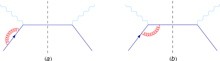
Figure 1.7: 1-loop virtual diagrams: (a) self-energy and (b) vertex correction.

The UV divergences are regulated with the introduction of the running coupling constant whose argument has to be of the order of the virtuality of the probing particle (the photon).

The IR divergences, on the other hand, originate when the incoming quark emits a gluon with vanishing 4-momentum (soft singularity), i.e., $z=1$, $\bar{z}=0$ and ${\boldsymbol{k}}=0$ in the quark Sudakov variables, or when the quark emits a collinear gluon. A corresponding term proportional to $\delta(1-z)$ has to be added to the quark-to-quark splitting function in Eq. (1.41)

$$P^{\text{\sf q}\text{\sf q}}(z)=C_{F}\left[{1+z^{2}\over 1-z}-\delta(1-z)\int_{0}^{1}{\rm d}y\;{1+y^{2}\over 1-y}\right]\;,$$ (1.55)

which reproduces the quark-to-quark splitting function in Tab. 1.1.

1.7.2 All order resummation of leading logarithms

To complete the resummation program, we should determine the LL contributions to all order in $\alpha_{\mathrm{s}}$. An accurate analysis of higher order diagrams shows that:

• in axial gauges, the real emission diagrams contributing in LL approximation are the ladder type ones like in Fig. 1.8;

• the phase space region generating large $\ln Q^{2}$ corresponds, in the Sudakov variables of the internal particles

  $$k_{i}=z_{i}\hat{p}{}+\bar{z}_{i}q^{\prime}+{\boldsymbol{k}}_{i}\;,$$ (1.56)

  to ordered transverse momenta

  $$Q^{2}>{\boldsymbol{k}}_{1}^{2}>{\boldsymbol{k}}_{2}^{2}>\cdots{\boldsymbol{k}}_{n}^{2}>\lambda^{2}\;,$$ (1.57)

  in fact, the $j$-th internal parton plays the role of the virtual photon in regard to the lower part of the diagram, so that the arguments of Sec. 1.7.1 can be repeated showing that the integration for ${\boldsymbol{k}}_{j+1}^{2}>{\boldsymbol{k}}_{j}^{2}$ is suppressed;

• the virtual contributions in LL approximation corresponds to vertex and self-energy corrections to the ladder diagrams;

• in addition to $\text{\sf g}\to\text{\sf q}$ and $\text{\sf q}\to\text{\sf q}$ splitting, we find $\text{\sf g}\to\text{\sf g}$ and $\text{\sf q}\to\text{\sf g}$ processes involving collinear singularities;

• the mass-shell constraints of the outgoing partons forces the $z_{j}$ variables to be ordered along the ladder:

  $$\hat{x}{}\simeq z_{1}<z_{2}<\cdots<z_{n}<1\;,$$ (1.58)

  while the $\bar{z}_{i}$ components in the ordered transverse momenta region (1.57) are very small.

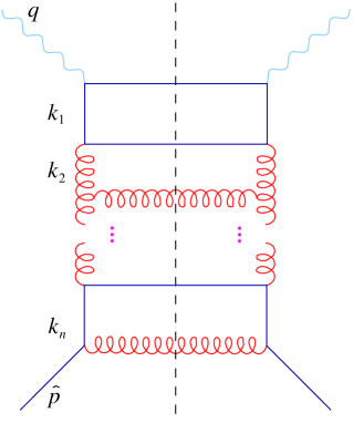
Figure 1.8: Ladder-type diagram contributing to DIS in the leading logarithmic approximation.

The $n$-loop contribution to the partonic tensor is

$$\alpha_{\mathrm{s}}^{n}\hat{W}{}_{\mu\nu}^{(\text{\sf a},n)}(\hat{p}{},q)= \sum_{\text{\sf a}_{1}}e_{\text{\sf a}_{1}}^{2}\Gamma_{\mu\nu}(\hat{x}{}\hat{p}{},q)\,A^{(n)}(Q^{2})\,{1\over\hat{x}{}}B^{(\text{\sf a}_{1}\text{\sf a},n)}(\hat{x}{})$$ (1.59a)

$$A^{(n)}(Q^{2})\,\raisebox{0.37pt}{:}= \int_{\lambda^{2}}^{Q^{2}}{{\rm d}{\boldsymbol{k}}_{1}^{2}\over{\boldsymbol{k}}_{1}^{2}}\alpha_{\mathrm{s}}({\boldsymbol{k}}_{1}^{2})\int_{\lambda^{2}}^{{\boldsymbol{k}}_{1}^{2}}{{\rm d}{\boldsymbol{k}}_{2}^{2}\over{\boldsymbol{k}}_{2}^{2}}\alpha_{\mathrm{s}}({\boldsymbol{k}}_{2}^{2})\cdots\int_{\lambda^{2}}^{{\boldsymbol{k}}_{n-1}^{2}}{{\rm d}{\boldsymbol{k}}_{n}^{2}\over{\boldsymbol{k}}_{n}^{2}}\alpha_{\mathrm{s}}({\boldsymbol{k}}_{n}^{2})$$ (1.59b)

$${1\over\hat{x}{}}B^{(\text{\sf a}_{1}\text{\sf a},n)}(\hat{x}{})\,\raisebox{0.37pt}{:}= \sum_{\text{\sf a}_{2}\cdots\text{\sf a}_{n}}\int_{0}^{1}{{\rm d}z_{1}\over z_{1}}\delta\big{(}1-{\hat{x}{}\over z_{1}}\big{)}\left[\prod_{j=2}^{n}\int_{z_{j-1}}^{1}{{\rm d}z_{j}\over z_{j}}\;{1\over 2\pi}P^{\text{\sf a}_{j-1}\text{\sf a}_{j}}\big{(}{z_{j-1}\over z_{j}}\big{)}\right]{1\over 2\pi}P^{\text{\sf a}_{n}\text{\sf a}}(z_{n})$$ (1.59c)

By summing over all $n\in{\mathbb{N}}$ and integrating over $\xi$ with the partonic densities just like in Eq. (1.44) we obtain, for the SF,

$$F_{i}(x,Q^{2})=\sum_{\text{\sf a},\text{\sf a}_{1}}\hat{F}_{i,\omega}^{(\text{\sf a}_{1})}\int_{0}^{1}{\rm d}\xi\;\sum_{n=0}^{\infty}A^{(n)}(Q^{2})B^{(\text{\sf a}_{1}\text{\sf a},n)}\big{(}{x\over\xi}\big{)}f^{(\text{\sf a})}(\xi)\qquad(i=2,L)\;,$$ (1.60)

where, from Eqs. (1.6) and (1.21), $\hat{F}_{2,\omega}^{(\text{\sf a}_{1})}=e_{\text{\sf a}_{1}}^{2}$ and $\hat{F}_{L,\omega}^{(\text{\sf a}_{1})}=0$.

The integral over transverse momenta can be performed by introducing the variable

$$L(Q^{2})\,\raisebox{0.37pt}{:}=\int_{\lambda^{2}}^{Q^{2}}{{\rm d}k^{2}\over k^{2}}\;\alpha_{\mathrm{s}}(k^{2})={1\over b_{0}}\ln{\alpha_{\mathrm{s}}(\lambda^{2})\over\alpha_{\mathrm{s}}(Q^{2})}$$ (1.61)

and gives

$$A^{(n)}(Q^{2})={1\over n!}L^{n}(Q^{2})\;.$$ (1.62)

By performing a Laplace transformation with respect to L, we obtain

$$A^{(n)}_{\rho}\,\raisebox{0.37pt}{:}=\int_{0}^{\infty}{\rm d}\rho\;A^{(n)}(L){\rm e}^{-\rho L}={1\over\rho^{n+1}}\;.$$ (1.63)

The integral over $z_{j}$ variables is easily evaluated in Mellin space by defining

$$B_{\omega}^{(\text{\sf a}_{1}\text{\sf a},n)}\,\raisebox{0.37pt}{:}= \int_{0}^{1}{\rm d}z\;z^{\omega-1}\,B^{(\text{\sf a}_{1}\text{\sf a},n)}(z)$$

$$= \sum_{\text{\sf a}_{2}\cdots\text{\sf a}_{n}}\gamma^{\text{\sf a}_{1}\text{\sf a}_{2}}_{\omega}\cdots\gamma^{\text{\sf a}_{n-1}\text{\sf a}_{n}}_{\omega}\gamma^{\text{\sf a}_{n}\text{\sf a}}_{\omega}=\big{[}{\boldsymbol{\gamma}}_{\omega}^{n}\big{]}^{\text{\sf a}_{1}\text{\sf a}}\;,$$ (1.64)

so that

$$F_{i,\omega,\rho}= \sum_{\text{\sf a},\text{\sf a}_{1}}\hat{F}_{i,\omega}^{(\text{\sf a}_{1})}\sum_{n=0}^{\infty}A^{(n)}_{\rho}B^{(\text{\sf a}_{1}\text{\sf a},n)}_{\omega}f^{(\text{\sf a})}_{\omega}$$

$$= \sum_{\text{\sf a},\text{\sf a}_{1}}\hat{F}_{i,\omega}^{(\text{\sf a}_{1})}\sum_{n=0}^{\infty}{1\over\rho}\left({{\boldsymbol{\gamma}}_{\omega}\over\rho}\right)^{n}_{\text{\sf a}_{1}\text{\sf a}}f^{(\text{\sf a})}_{\omega}$$

$$= \sum_{\text{\sf a},\text{\sf a}_{1}}\hat{F}_{i,\omega}^{(\text{\sf a}_{1})}\big{[}(\rho-{\boldsymbol{\gamma}}_{\omega})^{-1}\big{]}^{\text{\sf a}_{1}\text{\sf a}}f^{(\text{\sf a})}_{\omega}\;.$$ (1.65)

In $(\omega,\rho)$-space, the above results can be summarized in the following diagrammatic rules:

By inverting the Laplace transform we obtain

$$F_{i,\omega}(Q^{2})\,\raisebox{0.37pt}{:}=\int_{c-{\rm i}\infty}^{c+{\rm i}\infty}{{\rm d}\rho\over 2\pi{\rm i}}\;{\rm e}^{\rho L}\,F_{i,\omega,\rho}=\sum_{\text{\sf a},\text{\sf a}_{1}}\hat{F}_{i,\omega}^{(\text{\sf a}_{1})}\exp\{{\boldsymbol{\gamma}}_{\omega}L\}^{\text{\sf a}_{1}\text{\sf a}}f^{(\text{\sf a})}_{\omega}\;.$$ (1.66)

By splitting the exponential factor

$$\exp\{{\boldsymbol{\gamma}}L\}=\left[{\alpha_{\mathrm{s}}(\lambda^{2})\over\alpha_{\mathrm{s}}(Q^{2})}\right]^{{\boldsymbol{\gamma}}/b_{0}}=\left[{\alpha_{\mathrm{s}}(\mu_{F}^{2})\over\alpha_{\mathrm{s}}(Q^{2})}\right]^{{\boldsymbol{\gamma}}/b_{0}}\left[{\alpha_{\mathrm{s}}(\lambda^{2})\over\alpha_{\mathrm{s}}(\mu_{F}^{2})}\right]^{{\boldsymbol{\gamma}}/b_{0}}$$ (1.67)

and redefining the bare parton densities

$$f_{\omega}^{(\text{\sf a})}(\mu_{F}^{2})\,\raisebox{0.37pt}{:}=\sum_{\text{\sf b}}\left[{\alpha_{\mathrm{s}}(\lambda^{2})\over\alpha_{\mathrm{s}}(\mu_{F}^{2})}\right]^{{\boldsymbol{\gamma}}/b_{0}}_{\text{\sf a}\text{\sf b}}f_{\omega}^{(\text{\sf b})}\;,$$ (1.68)

we get an expression for the SF free of singularities which is the $\omega$-space analogue of Eq. (1.49). The moments of the $Q^{2}$-dependent PDF are defined by

$$f_{\omega}^{(\text{\sf a})}(Q^{2})\,\raisebox{0.37pt}{:}=\sum_{\text{\sf b}}\left[{\alpha_{\mathrm{s}}(\mu_{F}^{2})\over\alpha_{\mathrm{s}}(Q^{2})}\right]^{{\boldsymbol{\gamma}}/b_{0}}_{\text{\sf a}\text{\sf b}}f_{\omega}^{(\text{\sf b})}(\mu_{F}^{2})\;,$$ (1.69)

in terms of which we finally obtain

$$F_{i,\omega}(Q^{2})=\sum_{\text{\sf a}}\hat{F}_{i,\omega}^{(\text{\sf a})}\,f_{\omega}^{(\text{\sf a})}(Q^{2})\;,$$ (1.70)

i.e., in $x$-space, Eq. (1.51).

The evolution equation for the PDF, obtained by differentiating Eq. (1.69) with respect to $\ln Q^{2}$ reads

$${{\rm d}\over{\rm d}\ln Q^{2}}f^{(\text{\sf a})}_{\omega}(Q^{2})=\alpha_{\mathrm{s}}(Q^{2})\sum_{\text{\sf b}}\gamma_{\omega}^{\text{\sf a}\text{\sf b}}f^{(\text{\sf b})}_{\omega}(Q^{2})\qquad(\text{\sf a}=\text{\sf f},\bar{\text{\sf f}},\text{\sf g})\;.$$ (1.71)

The main differences of the resummed formula (1.71) with respect to the 1-loop one (1.52) are that (i) it has been obtained without approximations apart from the LL restrictions, (ii) the coupling is running and (iii) the evolution equation is extended to the gluon densities where $\gamma^{\text{\sf g}\text{\sf q}}$ and $\gamma^{\text{\sf g}\text{\sf g}}$ anomalous dimensions are present.

Chapter 2 Small-$\boldsymbol{x}$ hard processes

The coming of high energy colliders is making it possible to investigate strong interaction processes in very peculiar kinematic regimes, where the CM energy is much larger both than the hadronic masses and of the transferred momenta.

From a theoretical point of view, this new class of phenomena is of great importance by testing the asymptotic behaviour of cross sections in the high energy limit on one side and to check QCD theory in a much wider kinematic domain on the other side.

From the phenomenological point of view, the discovery of a marked rise of structure functions at HERA [12] has increased the interest of physicists for understanding the high energy features of QCD. What is actually observed (Fig. 2.1) is a surprising growth of the $F_{2}$ structure function towards low values of $x$. Note that $1/x$ is nearly proportional to the CM energy squared of the virtual photon-proton system

$$W^{2}\simeq{Q^{2}\over x}(1-x)\;\to\;{Q^{2}\over x}\qquad(x\ll 1)\;.$$

The growth is particularly marked for large values of $Q^{2}$, but it is also evident down to very low values (Fig. 2.2).

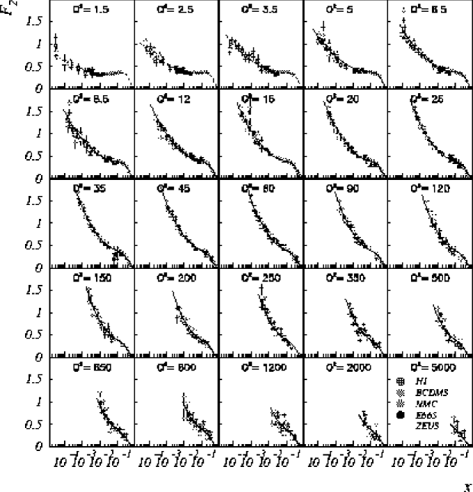
Figure 2.1: $x$-dependence of the $F_{2}$ structure function at different values of $Q^{2}$, showing the steep rise towards small-$x$ for all values of $Q^{2}$.

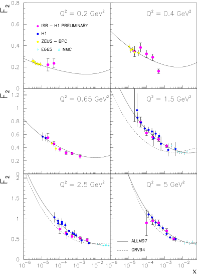
Figure 2.2: Small-$x$ rise of $F_{2}$ for very low values of $Q^{2}$.

In this chapter, after a brief introduction to Regge theory, we expose the general framework of the perturbative treatment of high energy inclusive strong interactions.

2.1 Regge behaviour

Before a fundamental theory for strong interactions — such as QCD — was established, the study of scattering of hadronic particles relied basically on rather general assumptions on the scattering matrix, such as Lorentz invariance, crossing symmetry, unitarity, causality, analyticity, asymptotic states etc.. The subsequent development led essentially to what is known as Regge theory [13], which determines the asymptotic behaviour of cross sections in the high energy limit regardless the strength of the coupling, i.e., independently of perturbation theory.

In this section we outline some important results of Regge theory which will be useful for our study on semi-hard processes. Keeping in mind our interest in high-energy inclusive reactions, unitarity allows us to relate the total cross section for the scattering of two initial particles “1” and “2” to the elastic scattering amplitude of the same particles. More precisely, by denoting with ${\mathcal{M}}^{\text{\sf a}_{1}\text{\sf a}_{1}^{\prime}}_{\text{\sf a}_{2}\text{\sf a}_{2}^{\prime}}(s,t)$ the scattering amplitude for the $s$-channel ($s>0,-s\leqslant t\leqslant 0$) process

$$(p_{1},\text{\sf a}_{1})+(p_{2},\text{\sf a}_{2})\to(p_{1}^{\prime},\text{\sf a}_{1}^{\prime})+(p_{2}^{\prime},\text{\sf a}_{2}^{\prime})\quad;\quad s\,\raisebox{0.37pt}{:}=(p_{1}+p_{2})\;,\;t\,\raisebox{0.37pt}{:}=(p_{1}-p_{1}^{\prime})\;,$$

($\text{\sf a}_{j}$ labelling the discrete quantum numbers) the optical theorem states that

$$\sigma_{\text{tot}}^{\text{\sf a}_{1},\text{\sf a}_{2}}(p_{1},p_{2})(s)={1\over s}\operatorname{\Im\text{m}}{\mathcal{M}}^{\text{\sf a}_{1}\text{\sf a}_{1}}_{\text{\sf a}_{2}\text{\sf a}_{2}}(s,t=0)\;.$$ (2.1)

Consider on the contrary the $t$-channel ($t>0,-t\leqslant s\leqslant 0$) process

$$(p_{1},\text{\sf a}_{1})+(-p_{1}^{\prime},\bar{\text{\sf a}}{}_{1}^{\prime})\to(-p_{2},\bar{\text{\sf a}}_{2})+(p_{2}^{\prime},\text{\sf a}_{2}^{\prime})\;,$$

where the antiparticle $\bar{\text{\sf a}}_{2}$ of “2” is now outgoing and the antiparticle $\bar{\text{\sf a}}{}_{1}^{\prime}$ of “1${}^{\prime}\,$” is incoming. By exploiting the crossing symmetry and the analyticity properties of the amplitude, we can say that the corresponding amplitude is given by the same function ${\mathcal{M}}^{\text{\sf a}_{1}\text{\sf a}_{1}^{\prime}}_{\text{\sf a}_{2}\text{\sf a}_{2}^{\prime}}(s,t)$, or better, by its analytic continuation from the $s$-channel to the $t$-channel region.

In the $t$-channel CM frame ($\vec{p}_{1}-\vec{p}_{1}{}^{\prime}=0$), the scattering angle $\theta$ between $\vec{p}_{1}$ and $-\vec{p}_{2}$ is given by

$$\cos\theta=1+{2s\over t}\quad;\quad-1\leqslant\cos\theta\leqslant 1\;.$$ (2.2)

By expressing the scattering amplitude by means of $(\cos\theta,t)$ instead of $(s,t)$, it is easy to perform the expansion in series of Legendre functions

$${\mathcal{M}}(s,t)=M(\cos\theta,t)=16\pi\sum_{l=0}^{\infty}(2l+1)M_{l}(t)P_{l}(\cos\theta)$$ (2.3)

which is called the partial wave series for ${\mathcal{M}}$.

We know from quantum mechanics that $P_{l}(\cos\theta)$ is the emission pattern of a state whose total angular momentum (in the CM system) is $l$. Hence we interpret the partial wave amplitude $M_{l}(t)$ as the contribution to the total amplitude corresponding to the $l^{\text{th}}$ angular momentum component.

Coming back to the $s$-channel domain, $|\cos\theta|>1$ loses its physical meaning. Nonetheless, thanks to analyticity, the contribution from the $l^{\text{th}}$ partial wave amplitude is still

$$16\pi(2l+1)M_{l}(t)P_{l}\big{(}1+{2s\over t}\big{)}\;.$$

In the high energy limit $s\gg|t|$ it holds

$$P_{l}\big{(}1+{2s\over t}\big{)}\to{\Gamma(2l+1)\over 2^{l}\Gamma^{2}(l+1)}\left({s\over t}\right)^{l}$$ (2.4)

which indicates a power-like behaviour in $s$ for the elastic scattering amplitude whose power equals the angular momentum of the state mediating the interaction. Moreover, the leading contribution to the amplitude will be given by the highest spin intermediate state allowed in the $t$-channel process.

As far as the differential cross section is concerned, we have ($Q^{2}=-t$)

$${{\rm d}\sigma\over{\rm d}Q^{2}}={1\over 16\pi}{|{\mathcal{M}}(s,-Q^{2})|^{2}\over s^{2}}\sim s^{2l-2}\;.$$ (2.5)

At this point we can anticipate that, in QCD, the leading contributions to cross sections will be given by gluon exchanges in the $t$-channel. In fact, $s$ and $u$ channel exchanges are suppressed by the large denominators $1/s$ and $1/u$ of the virtual particle propagators with respect to $t$-channel ones which involve $1/t$ ($s\simeq|u|\gg|t|$); the highest spin field in the QCD Lagrangian is the spin 1 gluon which, according to Eq. (2.5) is responsible of nearly constant differential cross sections.

What we have sketched are nothing but rough estimates, which give us an idea about the “order of magnitude” of the phenomena we are investigating. It is possible to push further the partial wave analysis in a beautiful mathematical description where the amplitudes $M_{l}(t)$ are analytically continued to complex values of the angular momentum variable $l$.

The complex functions $l\mapsto M_{l}(t)$ may present poles or branch cuts whose positions $\alpha_{i}(t)$ are smooth functions of $t$. Having in mind the $t$-channel process ($t>0$), we expect the amplitude to have a pole corresponding to the exchange of a physical particle of spin $J$ and mass $m$, thus $\exists i:\alpha_{i}(m^{2})=J$. It turns out that the functions $t\mapsto\alpha_{i}(t)$, which are called Regge trajectories, assume physical (semi)integer values when $t$ equals the squared mass of a particle or of a resonance. For each set of quantum numbers (except spin!) there is a definite Regge trajectory along which hadronic particles carrying those quantum numbers lie.

However also non-physical value of $\alpha_{i}(t)$ are important: each Regge trajectory contributes to the scattering amplitude in the $s$-channel. The kind of contribution depends on the particular nature of the singularity associated to the trajectory, e.g.,

$$M_{l}(t)\sim{1\over[l-\alpha(t)]^{\beta(t)}}\;\longleftrightarrow\;{\mathcal{M}}(s,t)\sim s^{\alpha(t)}[\ln s]^{\beta(t)-1}\;.$$ (2.6)

as if a particle of “effective spin” $\alpha(t)$ were exchanged. We are not surprised to encounter logarithmic corrections to the naïve power-like estimates: these are normal features in interacting theories.

According to the optical theorem, we argue the total cross section to be expressed — apart from logarithmic corrections — as a sum of powers of $s$ involving the intercepts of the various Regge trajectories:

$$\sigma_{\text{tot}}(s)=\sum_{i}c_{i}\,s^{\alpha_{i}(0)-1}\;\overset{s\to\infty}{\sim}\;c_{M}s^{\alpha_{M}(0)-1}\;,$$ (2.7)

where $\alpha_{M}(0)$ is the largest among the intercepts.

A careful analysis carried out from Froissart, based on general grounds and which assumes a small range force (as the strong interaction is) shows that unitarity limits the asymptotic behaviour of the scattering amplitude, setting an upper bound on the largest $s$-growth exponent: $\alpha_{M}(0)-1\leqslant 0$, i.e., the total cross section of any reaction cannot grow faster than some power of $\ln s$.

In this connection the phenomenological analysis seems to present a sort of puzzle: a Regge inspired fit like Eq. (2.7) with two terms ($i=1,2$), as performed by Donnachie and Landshoff [14], describe very well the experimental data, with the same Reggeon intercepts $\alpha_{\mathbb{R}}(0)-1=-0.45$ and $\alpha_{\mathbb{P}}(0)-1=0.08$ for different processes (see Fig. 2.3). However, the latter clearly violates the Froissart bound. The answer to this apparent paradox has to be found in the kinematic domain so far investigated which is evidently outside the regime where unitarity effects become important.

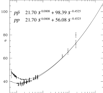
Figure 2.3: The Donnachie-Landshoff fit to (a) proton-proton and antiproton-proton and (b) to photon-proton total cross section.

Anyway, there is evidence of a dominance of Regge-particles in the high energy region so far investigated. The lower Regge trajectory $\alpha_{\mathbb{R}}$ corresponds to the family of particles including the $\rho$, $\omega$, etc. mesons, and has odd parity and charge conjugation. This is the reason of the different coefficient $c_{\mathbb{R}}$ in the $pp$ and $p\bar{p}$ cross sections.

The upper trajectory does not distinguish charge conjugated particles — it has the quantum number of the vacuum — and does not correspond to any particle till now observed. This elusive particle has been given the name of pomeron and is the responsible of the high energy behaviour of cross sections, at least before the unitarity regime, where pomeron self-interactions are no longer negligible.

Is perturbative QCD able to describe the pomeron? and, in general, the high energy processes? These are the questions we wish to give an answer.

2.2 Perturbative analysis of DIS in leading $\boldsymbol{\ln 1/x}$
approximation

We are ready to start the analysis of DIS in the high energy limit $s\gg Q^{2}\gg\Lambda^{2}$, i.e., from Eq. (A.13), $xy\ll 1$. In particular, we are interested in the kind of process where $x\ll 1$ and $y\ll 1$.

The large virtuality $Q^{2}\gg\Lambda^{2}$ of the virtual photon should justify the use of perturbation theory, regardless of the value of $s$. However, in this regime where there are two very different hard scales, the QCD perturbative expansion is affected by large coefficients which, to order $\alpha_{\mathrm{s}}^{n}$ and for inclusive observables, are ${\mathcal{O}}[(\ln W^{2}/Q^{2})^{m}]\sim\ln^{m}1/x:m\leqslant n$. We have to face again a resummation problem, this time with respect to the effective expansion parameter $\alpha_{\mathrm{s}}\ln 1/x$ which can be of the order of unity for small values of $x$ even if $\alpha_{\mathrm{s}}\ll 1$. The leading $\ln 1/x$ (L$x$) approximation consists in taking into account all the perturbative terms of order $[\alpha_{\mathrm{s}}\ln 1/x]^{n}$, the next-to-leading $\ln 1/x$ (NL$x$) considers all contributions like $\alpha_{\mathrm{s}}[\alpha_{\mathrm{s}}\ln 1/x]^{n}$ and so on.

In order to resum the leading logarithms of $x$ a technique is usually adopted which is in certain aspects similar to the one employed in the resummation of the leading $\ln Q^{2}$. First of all, the collinear factorization formula for SF has to be replaced with a corresponding high energy (${\boldsymbol{k}}$-dependent) factorization [15]. The latter should take into account the larger phase space available and should generalize the former. The second step is to calculate the evolution (in $x$-space) of the “parton density” factor which obey an equation obtained by Balitskiĭ, Fadin, Kuraev and Lipatov (BFKL) [16]. By performing the transverse-space integration of the parton densities with the partonic cross section, which can be explicitly evaluated, one obtains a factorized expression for the high energy (small-$x$) SF where both partonic SF and PDF are resummed.

2.2.1 High energy factorization

As we noticed in Sec. 2.1 and we shall show in more detail in Sec. 2.3, the terms contributing to the L$x$ approximation arise from gluon exchanges in the $t$-channel. Since gluons can couple to the (virtual) photon only via quarks, we are led to consider diagrams where single gluon (Fig. 2.4a) and multiple gluon (Fig. 2.4b) exchanges are possible.

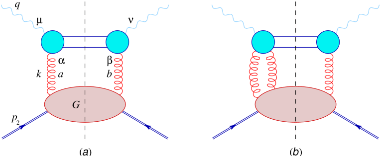
Figure 2.4: Single (a) and multiple (b) gluon exchanges in the high energy limit of photon-proton total cross section.

If we work in axial gauges, the multiple gluon exchange diagrams are suppressed by powers of $\alpha_{\mathrm{s}}(Q^{2})$, because the gluons’ endpoints have a very large relative velocity, the upper one being nearly collinear to $p_{1}$ and the lower one nearly collinear to $p_{2}$ (see Eq. (2.13)).

Single $t$-channel gluon exchanges in L$x$ approximation are then factorizable as we will briefly explain in the following. According to Eq. (A.4), the contribution to the hadronic tensor from Fig. 2.4a can be written

$$W^{\mu\nu}(p_{2},q)={1\over 4\pi}\int{{\rm d}^{4}k\over(2\pi)^{4}}\;\overset{ab}{A}{}^{\mu\nu}_{\alpha\beta}(q,k)\,\overset{ab}{G}{}^{\alpha\beta}(p_{2},k)$$ (2.8)

(summation over colour indices $a,b$ is understood) where

$$\overset{ab}{A}{}^{\mu\nu}_{\alpha\beta}(q,k)\,\raisebox{0.37pt}{:}=\int{\rm d}\Phi(p_{3},p_{4})\;\overset{\;a}{{\mathcal{M}}}{}^{\mu}_{\alpha}(q,k,p_{3},p_{4})\overset{\;b}{{\mathcal{M}}}{}^{\nu}_{\beta}(q,k,p_{3},p_{4})^{*}$$ (2.9)

denotes the lowest order $\text{\sf q}\bar{\text{\sf q}}$ contribution to the $\gamma^{*}\text{\sf g}^{*}\to\gamma^{*}\text{\sf g}^{*}$ absorptive part (Fig. 2.5) integrated over the final particle phase space and $\overset{ab}{G}{}^{\alpha\beta}(p_{2},k)$ is the full $p\text{\sf g}^{*}\to p\text{\sf g}$ absorptive part, including the gluon propagator.

$\overset{\;a}{{\mathcal{M}}}{}^{\mu}_{\alpha}\quad=\quad$

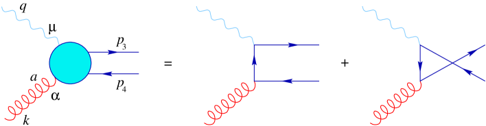
Figure 2.5: Feynman diagrams for photon-gluon coupling at lowest order in $\alpha_{\mathrm{s}}$.

In the high energy, small-$y$ regime, the differential cross section is essentially given by the $F_{2}$ structure function, and can be obtained by the eikonal approximation at the electron-photon vertex. The eikonal approximation can be applied when the components of the transferred momentum $q$ are much smaller than that of the external momenta $p_{1}$ and $p_{1}^{\prime}$; it consists in the replacement of the helicity conserving vertex $\bar{u}_{\sigma}(p_{1}^{\prime})\gamma^{\mu}u_{\sigma}(p_{1})\simeq 2p_{1}^{\mu}$ and neglecting the non conserving one, i.e., to approximate the leptonic tensor (A.3)

$$L_{\mu\nu}(p_{1},q)\simeq 2p_{1\mu}2p_{1\nu}\;.$$ (2.10)

After contraction with the hadronic tensor we obtain

$$2p_{1\mu}2p_{1\nu}\,W^{\mu\nu}=-Q^{2}F_{1}+2s{(1+y/2)^{2}\over y}F_{2}\simeq{2s\over y}F_{2}\qquad(y\ll 1)$$ (2.11)

and hence, using Eq. (A.13),

$$F_{2}\simeq 2x\big{(}{y\over Q}p_{1\mu}\big{)}\big{(}{y\over Q}p_{1\nu}\big{)}\int{{\rm d}^{4}k\over(2\pi)^{4}}\;\overset{ab}{A}{}^{\mu\nu}_{\alpha\beta}(q,k)\,{1\over 4\pi}\overset{ab}{G}{}^{\alpha\beta}(p_{2},k)$$ (2.12)

By adopting the Sudakov parametrization

$$q =yp_{1}+\bar{y}p_{2}+{\boldsymbol{q}}$$ (2.13a)

$$k =\bar{z}p_{1}+zp_{2}+{\boldsymbol{k}}$$ (2.13b)

the high energy limit constrains $\bar{y}\ll y\ll 1$ and it turns out that the dominant integration region in the $k$ variable is the one with fixed ${\boldsymbol{k}}^{2}$, $\bar{z}\ll z\ll 1$ and $|k^{2}|\simeq{\boldsymbol{k}}^{2}={\mathcal{O}}(yzs)={\mathcal{O}}({Q^{2}})$.

The next step is to show that only a single gluon polarization contributes in the diagram of Fig. 2.4a. Since the amplitude $\overset{\;a}{{\mathcal{M}}}{}^{\mu}_{\alpha}=\raisebox{0.37pt}{:}\hskip 3.0pt{\mathcal{M}}^{\mu}_{\alpha}\overset{a}{T}{}$ involves a colourless object (the photon), the tensor $\overset{ab}{A}{}^{\mu\nu}_{\alpha\beta}=\raisebox{0.37pt}{:}\hskip 3.0ptA^{\mu\nu}_{\alpha\beta}\delta^{ab}$ satisfies the Ward identities of electrodynamics

$$k^{\alpha}A^{\mu\nu}_{\alpha\beta}=k^{\beta}A^{\mu\nu}_{\alpha\beta}=0$$ (2.14)

and thus the following decomposition holds:

$$A_{\alpha\beta}\,\raisebox{0.37pt}{:}= \big{(}{y\over Q}p_{1\mu}\big{)}\big{(}{y\over Q}p_{1\nu}\big{)}A^{\mu\nu}_{\alpha\beta}(q,k)$$ (2.15a)

$$= A_{1}\left({k_{\alpha}k_{\beta}\over k^{2}}-g_{\alpha\beta}\right)-A_{2}{1\over k^{2}}\left(k_{\alpha}-{k^{2}\over qk}q_{\alpha}\right)\left(k_{\beta}-{k^{2}\over qk}q_{\beta}\right)$$ (2.15b)

where the dimensionless Lorentz invariant functions $A_{i}$ depends on $Q^{2}$, ${\boldsymbol{k}}^{2}$, $2qk\simeq yzs$, $2(yp_{1})k=yzs$ or, equivalently, on the rescaled variables $x/z$ and $Q^{2}/{\boldsymbol{k}}^{2}$.

In the kinematic regime mentioned above, the amplitudes $A_{1}$ and $A_{2}$ satisfy

$$A_{1}\simeq A_{2}\simeq{\mathcal{O}}\big{(}{x\over z}\big{)}$$

for fixed values of ${\boldsymbol{k}}^{2}/zs$ (they are exactly equal when $k^{2}=0$ in order to cancel the spurious pole at $k^{2}=0$ in Eq. (2.15)). This is due to the fact that the corresponding diagrams Fig. 2.5 involve quark (spin $1/2$) exchanges, vanishing like $s^{-1}\sim x$ for increasing energy (see Eq. (2.5)). Therefore, the dominant contribution in Eq. (2.12) is obtained for fixed values of $x/z={\mathcal{O}}(1)$ and hence $z\to 0$. On the other hand, when $z\to 0$, $k^{2}\simeq-{\boldsymbol{k}}^{2}$ and ${\boldsymbol{k}}^{2}/zs$ is fixed, the polarization tensor in front of $A_{2}$ can be replaced with

$$4\;{{\boldsymbol{k}}^{2}\over zs}\,{p_{1\alpha}p_{1\beta}\over s}\,{1\over z}\left[1+{\mathcal{O}}\big{(}z,{|{\boldsymbol{k}}|\over s}\big{)}\right]\;,$$ (2.16)

which clearly shows an $1/z$ enhancement factor with respect to the $A_{1}$ one and a “selection” of the gluon polarization along $p_{2}$.

By using Eqs. (2.15) and (2.16), Eq. (2.12) can be rewritten as

$$F_{2}=2x\int_{0}^{1}{{\rm d}z\over z}\int{\rm d}^{2}{\boldsymbol{k}}\int{{\rm d}k^{2}\over 2(2\pi)^{4}}\;{4{\boldsymbol{k}}^{2}\over z^{2}s^{2}}p_{1\alpha}p_{1\beta}\,A_{2}\,\delta^{ab}{\overset{ab}{G}{}^{\alpha\beta}\over 4\pi}\;.$$ (2.17)

By defining the off-shell partonic cross section

$$\hat{\sigma}_{2}\big{(}{x\over z},{Q^{2}\over{\boldsymbol{k}}^{2}}\big{)}\,\raisebox{0.37pt}{:}={2x\over z}A_{2}\big{(}{x\over z},{Q^{2}\over{\boldsymbol{k}}^{2}}\big{)}\simeq{2xz\over{\boldsymbol{k}}^{2}}p_{2}^{\alpha}p_{2}^{\beta}A_{\alpha\beta}$$ (2.18)

and the unintegrated gluon density

$$\mathcal{F}(z,{\boldsymbol{k}})\,\raisebox{0.37pt}{:}=\int{{\rm d}k^{2}\over(2\pi)^{5}}\;{{\boldsymbol{k}}^{2}\over zs^{2}}p_{1\alpha}p_{1\beta}\sum_{a}\overset{aa}{G}{}^{\alpha\beta}(p_{2},k)$$ (2.19)

the high energy, ${\boldsymbol{k}}$-dependent, factorization formula is established [15]:

$$F_{2}(x,Q^{2})=\int_{0}^{1}{{\rm d}z\over z}\int{\rm d}^{2}{\boldsymbol{k}}\;\hat{\sigma}_{2}\big{(}{x\over z},{Q^{2}\over{\boldsymbol{k}}^{2}}\big{)}\mathcal{F}(z,{\boldsymbol{k}})\;.$$ (2.20)

Eq. (2.18) shows that the hard partonic cross section $\hat{\sigma}_{2}$ is given by the diagram in Fig. (2.5) where the soft ($z\to 0$) off-shell gluon is coupled to an external fast quark (or gluon) with an eikonal vertex $p_{2}^{\alpha}$. It is important to note that $\hat{\sigma}_{2}$ is a gauge invariant object, despite the off-shellness of the “incoming” virtual gluon $k$. The reason for this is that the eikonal coupling induces physical polarization for the incoming gluon.

The formula (2.20) can be written in diagonal form in Mellin space. With the definitions of Eqs. (C.19) we get

$$F_{2,\omega}(Q^{2})=\int{\rm d}^{2}{\boldsymbol{k}}\;\hat{\sigma}_{\omega}\big{(}{Q^{2}\over{\boldsymbol{k}}^{2}}\big{)}\,{\mathcal{F}}_{\omega}({\boldsymbol{k}})$$ (2.21)

or, equivalently,

$$F_{2,\omega}(\gamma)=\hat{\sigma}_{\omega}(\gamma)\,{\mathcal{F}}_{\omega}(\gamma)\;.$$ (2.22)

2.2.2 Relation with the collinear factorization

The high energy factorization formula (2.20) is a generalization of the collinear one (1.5) which holds not only for $s\sim Q^{2}\gg\Lambda^{2}$ but also in the semi-hard regime $s\gg Q^{2}\gg\Lambda^{2}$. This can be easily seen if we remember that, for $s\sim Q^{2}$, the leading contributions to the cross section arise from emission of partons whose transverse momenta are strongly ordered. In particular, the integration over ${\boldsymbol{k}}$ is important only for ${\boldsymbol{k}}^{2}\ll Q^{2}$, where the hard cross section assume the typical form of collinear emission

$$\hat{\sigma}\big{(}\hat{x}{},{Q^{2}\over{\boldsymbol{k}}^{2}}\big{)}\simeq\sum_{\text{\sf a}\in\{\text{partons}\}}e_{\text{\sf a}}^{2}\,{{\alpha_{\mathrm{s}}\over 2\pi}}\ln{Q^{2}\over{\boldsymbol{k}}^{2}}\,\hat{x}{}P^{\text{\sf a}\text{\sf g}}(\hat{x}{})\qquad({\boldsymbol{k}}^{2}\ll Q^{2})\;.$$ (2.23)

In $\omega$-space this means that

$$F_{2,\omega}(Q^{2})=(\sum_{\text{\sf a}}e_{\text{\sf a}}^{2})\int^{Q^{2}}{\rm d}^{2}{\boldsymbol{k}}\;\alpha_{\mathrm{s}}\gamma^{\text{\sf q}\text{\sf g}}_{\omega}\ln{Q^{2}\over{\boldsymbol{k}}^{2}}{\mathcal{F}}_{\omega}({\boldsymbol{k}})\;.$$ (2.24)

Since ${1\over 2N_{\!f}}\sum_{\text{\sf a}}e_{\text{\sf a}}^{2}$ is just the partonic structure function for the quark singlet density, we identify

$$f_{\omega}^{(\Sigma)}(Q^{2})=\int^{Q^{2}}{\rm d}^{2}{\boldsymbol{k}}\;\alpha_{\mathrm{s}}\,2N_{\!f}\gamma^{\text{\sf q}\text{\sf g}}_{\omega}\ln{Q^{2}\over{\boldsymbol{k}}^{2}}{\mathcal{F}}_{\omega}({\boldsymbol{k}})\;.$$ (2.25)

Taking the derivative with respect to $\ln Q^{2}$ yields

$${{\rm d}\over{\rm d}\ln Q^{2}}f_{\omega}^{(\Sigma)}(Q^{2})= \alpha_{\mathrm{s}}\,2N_{\!f}\gamma^{\text{\sf q}\text{\sf g}}_{\omega}\int^{Q^{2}}{\rm d}^{2}{\boldsymbol{k}}\;{\mathcal{F}}_{\omega}({\boldsymbol{k}})$$ (2.26)

$$= \alpha_{\mathrm{s}}\,2N_{\!f}\gamma^{\text{\sf q}\text{\sf g}}_{\omega}f_{\omega}^{(\text{\sf g})}(Q^{2})$$

once we have made the further identification

$$f_{\omega}^{(\text{\sf g})}(Q^{2})=\int^{Q^{2}}{\rm d}^{2}{\boldsymbol{k}}\;{\mathcal{F}}_{\omega}({\boldsymbol{k}})\;.$$ (2.27)

In conclusion, ${\mathcal{F}}_{\omega}({\boldsymbol{k}})$ represents the unintegrated gluon density in ${\boldsymbol{k}}$-space which is related to the usual gluon PDF by Eq. (2.27). The former gives the most important contribution to the quark singlet density in the framework of high energy factorization.

However, when $s\gg Q^{2}$ we cannot exploit the collinear picture to describe the $Q^{2}$ evolution of the singlet density, since $\hat{\sigma}$ does not necessarily contain a leading $\ln Q^{2}$. Rather, $\hat{\sigma}$ has to be considered the ${\mathcal{O}}(\alpha_{\mathrm{s}})$ coefficient of the gluon density contributing to $F_{2}$. The ${\boldsymbol{k}}$-convolution of $\hat{\sigma}$ with the unintegrated gluon density provides the resummation of the large $\ln 1/x$ in the coefficient function, as we shall see in Sec. 2.3.3.

2.3 Resummation of $\boldsymbol{\ln 1/x}$ in the leading approximation

The high energy factorization formula (2.20) shows that the leading high energy contribution to semi-hard DIS is governed by the unintegrated gluon density for small values of the gluon momentum fraction $z$. As one can easily realize, it is not possible to determine perturbatively the gluon density, since long distance effects are unavoidable when dealing with hadrons. Nevertheless, in a particular regime (to be specified soon), the perturbative analysis allows us to extract information about the dependence of the unintegrated gluon density on the “hard” variables $z$ and ${\boldsymbol{k}}$ involved in the hard gluon-photon vertex. This is done by means of an evolution equation in $z$-space obtained more than twenty years ago by the russian school.

In this section we will go over the road that led to the BFKL equation [16]. The latter resums all the leading logarithmic ($\ln s$) coefficients of the $\alpha_{\mathrm{s}}$ perturbative series for inclusive semi-hard processes. The following presentation will be useful in order to identify the basic physical quantities (in connection with the DGLAP ones) and to fix the framework for the NL$x$ formulation of the BFKL equation (Cap. 3) and for its subsequent improvement (Chap. 4).

Following the idea of factorization of non perturbative effects, we can guess that the probability to find a gluon with momentum fraction $z$ with respect to the parent proton and transverse momentum ${\boldsymbol{k}}$ should be given by a convolution of bare partonic densities $f^{(\text{\sf a})}$ with a perturbative calculable function ${\mathcal{G}}^{(\text{\sf a})}$ which embodies all kinds of intermediate processes between the bare parton a and the hard gluon. At high energies, only gluon exchanges in the $t$-channel contribute in the L$x$ approximation. Therefore we assume a sort of factorized expression for the unintegrated gluon density of the form

$${\mathcal{F}}_{\omega}({\boldsymbol{k}})\simeq\int{\rm d}^{2}{\boldsymbol{k}}_{0}\;f_{\omega}^{(\text{\sf g})}({\boldsymbol{k}}_{0})\,{\mathcal{G}}_{\omega}({\boldsymbol{k}},{\boldsymbol{k}}_{0})$$ (2.28)

which stresses again the relevance of the transverse degrees of freedom. Here $f_{\omega}^{(\text{\sf g})}({\boldsymbol{k}}_{0})$ denotes the Mellin transform of the probability density of finding a gluon with transverse momentum ${\boldsymbol{k}}_{0}$ inside the proton; it is to be considered as an unknown input function to be eventually specified in particular phenomenological applications.

The function ${\mathcal{G}}_{\omega}({\boldsymbol{k}},{\boldsymbol{k}}_{0})$ is the basic object we wish to investigate; it will be extensively studied throughout this thesis.

2.3.1 Leading $\boldsymbol{\ln 1/x}$ BFKL equation

The function ${\mathcal{G}}_{\omega}({\boldsymbol{k}},{\boldsymbol{k}}_{0})$ represents the set of gluon exchanges contributing in L$x$ approximation to high energy scattering of two strong interacting objects. Also high energy scattering of colourless particles is governed by gluon exchanges: in this case the coupling to gluons occurs via quark or EW boson intermediate states.

In order to determine ${\mathcal{G}}_{\omega}$, the simplest situation we can consider is high energy scattering of two partons a and b.

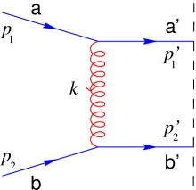
Figure 2.6: The lowest order Feynman diagram contributing to leading L$x$ order.

At Born level, the cross section is dominated by one gluon exchange in the $t$-channel (Fig. 2.6) corresponding to the amplitude

$${\mathcal{M}}_{2\to 2}^{(0)}=-{\rm i}\,2s\,\Gamma_{\text{\sf a}^{\prime}\text{\sf a}}^{r}\,{1\over t}\,\Gamma_{\text{\sf b}^{\prime}\text{\sf b}}^{r}\quad,\quad s=(p_{1}+p_{2})^{2}\quad,\quad t=(p_{1}-p_{1}^{\prime})^{2}$$ (2.29)

where summation over repeated colour indices is understood and the parton-gluon vertices are

$$\Gamma_{\text{\sf a}^{\prime}\text{\sf a}}^{r}\,\raisebox{0.37pt}{:}=g\,\delta_{\lambda_{\text{\sf a}^{\prime}}\lambda_{\text{\sf a}}}\,f^{a^{\prime}ra}\qquad(\text{\sf a}=\text{\sf g}=\text{gluon})\;,$$ (2.30a)

$$\Gamma_{\text{\sf a}^{\prime}\text{\sf a}}^{r}\,\raisebox{0.37pt}{:}=-{\rm i}g\,\delta_{\lambda_{\text{\sf a}^{\prime}}\lambda_{\text{\sf a}}}\,\overset{r}{T}{}_{\rm a^{\prime}a}\qquad(\text{\sf a}=\text{\sf q}=\text{quark})\;.$$ (2.30b)

Since gluon exchanges do not affect the flavour of the quarks and the polarization/helicity $\lambda_{\text{\sf a}^{\prime}}=\lambda_{\text{\sf a}}$ is conserved, only colour degrees of freedom and kinematics have to be taken into account. Note also that the longitudinal variables corresponding to the Sudakov decomposition $k=zp_{1}+\bar{z}p_{2}+{\boldsymbol{k}}$ are small in the high energy regime: $z=|\bar{z}|=|t|/s\ll 1$.

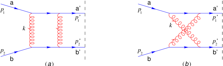
Figure 2.7: The two particle final states virtual correction diagrams contributing at leading L$x$ order. Iteration of gluon exchange in the $s$-channel (a) and in the $u$-channel (b).

The 1-loop virtual corrections to the elastic amplitude give rise to a $\ln s$ coefficient. In covariant gauges, only the “box” and “crossed” diagrams of Fig. 2.7 contributes with logarithms of $s$. These amplitudes can be projected in the subspaces of the irreducible representations of $8\otimes 8$ where the couple of exchanged gluon lives. In other words, a given amplitude can be considered as a sum of terms representing the exchange in the $t$-channel of colour structures belonging to the various $8\otimes 8$ irreducible representations. When summing the amplitudes ${\mathcal{M}}^{(1,s)}_{2\to 2}$ and ${\mathcal{M}}^{(1,u)}_{2\to 2}$ of Fig. 2.7a and b respectively, which kinematically corresponds to the replacement $s\leftrightarrow u$, only the octet representation of the antisymmetric part $(8\otimes 8)_{A}=1\oplus 8\oplus 10\oplus\overline{10}$ interferes constructively. For this reason the colour factors can be well represented by the parton-gluon vertices of Eqs. (2.30).

The octet part of ${\mathcal{M}}^{(1,s)}_{2\to 2}$ reads

$${\mathcal{M}}^{(1,s)}_{2\to 2}\cong g^{2}s^{2}N_{c}\,\Gamma_{\text{\sf a}^{\prime}\text{\sf a}}^{r}\,I(s,t)\,\Gamma_{\text{\sf b}^{\prime}\text{\sf b}}^{r}$$ (2.31)

where the loop integral $I$ yields

$$I(s,t)\simeq -{{\rm i}\over(2\pi)^{2}\,s\,t}\ln\big{(}-{s\over s_{0}}\big{)}\Omega^{(0)}(-t)$$ (2.32a)

$$\Omega^{(0)}({\boldsymbol{k}}^{2})\,\raisebox{0.37pt}{:}= -{{\boldsymbol{k}}^{2}\over 4\pi}\int{{\rm d}{\boldsymbol{q}}\over{\boldsymbol{q}}^{2}({\boldsymbol{k}}-{\boldsymbol{q}})^{2}}$$ (2.32b)

The logarithmic factor stems from integration over the longitudinal variables of $k$. In the massless theory the scale of the energy $s_{0}$ is of the order of the transverse momentum squared of the outgoing particles. In the L$x$ approximation, however, the choice of $s_{0}$ is irrelevant, because with an other choice $s^{\prime}_{0}$ the difference $\ln s/s_{0}-\ln s/s_{0}^{\prime}=\ln s^{\prime}_{0}/s_{0}$ is independent on $s$ and therefore subleading.

The coefficient $\Omega(-t)$ of the logarithmic term is an IR divergent two-dimensional integral. The IR divergence will cancel when considering real emission correction to the Born amplitude (see App. C.1).

We note that among the subleading 1-loop corrections we have neglected there are the self-energy and vertex-correction diagrams which determine the running of the coupling constant. Accordingly, in a L$x$ treatment of the radiative corrections, $\alpha_{\mathrm{s}}$ must be regarded as fixed.

By collecting Eqs. (2.29), (2.31) and (2.32) the full 1-loop expression for the elastic amplitude results

$$[{\mathcal{M}}^{(0)}+{\mathcal{M}}^{(1)}]_{2\to 2}=-{\rm i}\,2s\,\Gamma_{\text{\sf a}^{\prime}\text{\sf a}}^{r}\,{1+\bar{\alpha}_{\mathrm{s}}\Omega(-t)\ln(s/s_{0})\over t}\,\Gamma_{\text{\sf b}^{\prime}\text{\sf b}}^{r}\;.$$ (2.33)

Eq. (2.33) is intriguing, since the logarithmic correction looks like the $\bar{\alpha}_{\mathrm{s}}$ truncation of $(s/s_{0})^{\bar{\alpha}_{\mathrm{s}}\Omega(-t)}$ which would correspond to Regge behaviour. The 2-loop correction has been computed [16] and confirms this assumption. In conclusion, we make the ansatz that, in L$x$ approximation, the amplitude for elastic scattering with the gluon quantum numbers in the $t$-channel is

$${\mathcal{M}}_{2\to 2}=-{\rm i}\,2s\,\Gamma_{\text{\sf a}^{\prime}\text{\sf a}}^{r}\,{(s/s_{0})^{\bar{\alpha}_{\mathrm{s}}\Omega(-t)}\over t}\,\Gamma_{\text{\sf b}^{\prime}\text{\sf b}}^{r}$$ (2.34)

which states the reggeization of the gluon.

Upon colour averaging and by using the phase space measure for two particle final states (including the flux factor $(2s)^{-1}$)

$${\rm d}\phi^{(2)}=\frac{1}{(4\pi)^{2}}\,\frac{1}{s^{2}}\,{\rm d}{\boldsymbol{k}}\;,$$ (2.35)

Eq. (2.34) yields the two-particle final state contribution to the differential cross section

$${\rm d}\sigma_{\text{\sf a}\text{\sf b}\to 2}=h_{\text{\sf a}}^{(0)}({\boldsymbol{k}})\left({s\over s_{0}}\right)^{\bar{\alpha}_{\mathrm{s}}2\Omega(-t)}h_{\text{\sf b}}^{(0)}({\boldsymbol{k}})\,{\rm d}{\boldsymbol{k}}$$ (2.36)

in terms of the Born impact factors

$$h_{\text{\sf a}}^{(0)}({\boldsymbol{k}})\,\raisebox{0.37pt}{:}={2\alpha_{\mathrm{s}}C_{\text{\sf a}}\over\sqrt{N_{c}^{2}-1}}\,{1\over{\boldsymbol{k}}^{2}}\quad;\quad C_{\text{\sf g}}=C_{A}\quad;\quad C_{\text{\sf q}}=C_{F}\;.$$ (2.37)

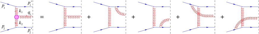
Figure 2.8: The Lipatov effective vertex for the emission of a real gluon: the blob represents gluon emission both from the exchanged gluon and from the external particles.

Let’s now consider the 1-loop order real emission corrections. At L$x$ level, the high-energy kinematics favours the emission of an additional gluon (Fig. 2.8) of momentum $q_{1}$ and polarization $\epsilon$ in the central region $q_{1}^{+}\sim q_{1}^{-}\sim|{\boldsymbol{q}}_{1}|$ . The corresponding amplitude is

$${\mathcal{M}}^{(0)}_{2\to 3}= -{\rm i}\,2s\,\Gamma_{\text{\sf a}^{\prime}\text{\sf a}}^{r_{1}}\,{1\over t_{1}}\Upsilon^{c}_{r_{1}r_{2}}{1\over t_{2}}\,\Gamma_{\text{\sf b}^{\prime}\text{\sf b}}^{r_{2}}\;,$$ (2.38)

$$\Upsilon^{c}_{r_{1}r_{2}}(k_{1},k_{2})\,\raisebox{0.37pt}{:}=\,{\rm i}g\,f^{r_{1}c\,r_{2}}\,\overset{*}{\epsilon}{}_{\mu}(q_{1})J^{\mu}(k_{1},k_{2})\;,$$ (2.39)

where $q_{1}^{\mu}=k_{1}^{\mu}-k_{2}^{\mu}$, $t_{i}=k_{i}^{2}\simeq-{\boldsymbol{k}}_{i}^{2}$ and

$$J^{\mu}(k_{1},k_{2})=-({\boldsymbol{k}}_{1}+{\boldsymbol{k}}_{2})^{\mu}+p_{1}^{\mu}\left({2p_{2}k_{1}\over s}+{{\boldsymbol{k}}_{1}^{2}\over p_{1}k_{2}}\right)+p_{2}^{\mu}\left({2p_{1}k_{2}\over s}+{{\boldsymbol{k}}_{2}^{2}\over p_{2}k_{1}}\right)$$ (2.40)

is the Lipatov effective vertex.

The 1-loop virtual corrections contributing to the three-particle final states in L$x$ approximation can be computed, and their final effect — according to gluon reggeization — consists simply in the replacement of the propagators

$${1\over t_{i}}\;\longrightarrow\;{1\over t_{i}}\left({s_{i}\over s_{0}}\right)^{\bar{\alpha}_{\mathrm{s}}\Omega(-t_{i})}\quad,\quad s_{i}=(q_{i}+q_{i-1})^{2}\qquad(i=1,2)\;.$$ (2.41)

in the amplitude (2.38).

After polarization and colour averaging, by using the three-body phase space measure ($z_{1}$ being the momentum fraction of $k_{1}$ with respect to $p_{1}$)

$${\rm d}\phi^{(3)}=\frac{1}{\pi(4\pi)^{4}}\,\frac{{\rm d}z_{1}\,{\rm d}{\boldsymbol{k}}_{1}\,{\rm d}{\boldsymbol{k}}_{2}}{s^{2}z_{1}}$$ (2.42)

and the properties of the $J$ vertex

$$q^{\mu}J_{\mu}(k_{1},k_{2})=0\quad\Longrightarrow\quad\sum_{\lambda}\overset{*}{\epsilon}{}^{\mu}_{\lambda}\epsilon^{\nu}_{\lambda}J_{\mu}J_{\nu}=-J^{2}=4{{\boldsymbol{k}}_{1}^{2}{\boldsymbol{k}}_{2}^{2}\over{\boldsymbol{q}}^{2}}$$ (2.43)

we obtain the three-particle final state contribution to the differential cross section

$${\rm d}\sigma_{\text{\sf a}\text{\sf b}\to 3}=h_{\text{\sf a}}({\boldsymbol{k}}_{1})\left({s_{1}\over s_{0}}\right)^{\bar{\alpha}_{\mathrm{s}}2\Omega(-t_{1})}\frac{\bar{\alpha}_{\mathrm{s}}}{\pi{\boldsymbol{q}}^{2}}\left({s_{2}\over s_{0}}\right)^{\bar{\alpha}_{\mathrm{s}}2\Omega(-t_{2})}h_{\text{\sf b}}({\boldsymbol{k}}_{2})\,{{\rm d}z_{1}\over z_{1}}\,{\rm d}{\boldsymbol{k}}_{1}\,{\rm d}{\boldsymbol{k}}_{2}$$ (2.44)

whose leading logarithmic character follows from the $z_{1}$ integration with infrared boundary $z_{1}>s_{0}/s$ (pure phase space would yield $\frac{{\boldsymbol{q}}^{2}}{s}<z_{1}<1-\frac{{\boldsymbol{k}}_{1}^{2}}{s}$).

To summarize the results till now obtained

• the huge part of the cross section arise from $t$-channel small virtualities gluon exchanges;

• the longitudinal phase space grows logarithmically with $s$ and the differential cross section is almost independent of the longitudinal variables (apart in the proximity of their upper boundary) whose integration yields just the $\ln s$ term;

• most of the longitudinal phase space corresponds to small values of the $z_{i}$ Sudakov variables;

• the mass-shell conditions of the outgoing particles causes the transverse momenta of the exchanged (reggeized) gluons to be the only relevant degrees of freedom for the amplitudes, furthermore $k_{i}^{2}\simeq-{\boldsymbol{k}}_{i}^{2}$.

Going to higher order in $\bar{\alpha}_{\mathrm{s}}$ is then straightforward.

Figure 2.9: The $n+2$ final particle gluon ladder contributing at L$x$ to high energy scattering. The thick wavy line represents reggeized gluon exchanges.

The scattering amplitude with $2+n$ particles in the final state receives its L$x$ contribution in the phase space region where the outgoing particles are strongly ordered in rapidity. At tree level, this corresponds to (half) a gluon ladder (Fig. 2.9) in multi-Regge kinematics (MRK):

$$k_{i}=z_{i}p_{1}+\bar{z}_{i}p_{2}+{\boldsymbol{k}}_{i}\qquad(i=1,\dots,n+1)$$ (2.45a)

$$1\equiv z_{0}\gg z_{1}\gg\cdots\gg z_{n+1}={-t_{n+1}\over s}$$ (2.45b)

$${t_{1}\over s}=\bar{z}_{1}\ll\bar{z}_{2}\ll\cdots\ll\bar{z}_{n+1}\ll 1$$ (2.45c)

where the squared transferred momenta $t_{i}=k_{i}^{2}\simeq-{\boldsymbol{k}}_{i}^{2}$ are of the same order and much smaller than $s$. Because of the mass-shell constraints and total momentum conservation, we can take $\{z_{i}:i=1,\dots,n\}$ and $\{{\boldsymbol{k}}_{j}:j=1,\cdots,n+1\}$ as independent variables; accordingly the phase space measure reads

$${\rm d}\phi^{(2+n)}={1\over s^{2}\,(4\pi)^{2n+2}\pi^{n}}\prod_{i=1}^{n}{{\rm d}z_{i}\over z_{i}}\prod_{j=1}^{n+1}{\rm d}{\boldsymbol{k}}_{j}\;.$$ (2.46)

The real emission amplitude is nothing but the generalization of Eq. (2.38), where outgoing gluons are coupled to internal lines by the effective vertex (2.40). Finally, the virtual corrections provides the reggeization of the exchanged gluons with the replacement of the propagators as in Eq. (2.41), yielding [16, 17]

$${\mathcal{M}}_{2\to 2+n}=-{\rm i}\,2s\,\Gamma_{\text{\sf a}^{\prime}\text{\sf a}}^{r_{1}}\,{(s_{1}/s_{0})^{\bar{\alpha}_{\mathrm{s}}\Omega_{1}}\over t_{1}}\Upsilon^{c_{1}}_{r_{1}r_{2}}{(s_{2}/s_{0})^{\bar{\alpha}_{\mathrm{s}}\Omega_{2}}\over t_{2}}\cdots\Upsilon^{c_{n}}_{r_{n}r_{n+1}}{(s_{n+1}/s_{0})^{\bar{\alpha}_{\mathrm{s}}\Omega_{n+1}}\over t_{n+1}}\,\Gamma^{r_{n+1}}_{\text{\sf b}{}^{\prime}\text{\sf b}}$$ (2.47)

with the shorthand notation $\Omega_{i}\equiv\Omega(-t_{i})$.

Having so obtained the $2+n$ particle differential cross section

$${\rm d}\sigma_{\text{\sf a}\text{\sf b}\to 2+n}=h_{\text{\sf a}}({\boldsymbol{k}}_{1})h_{\text{\sf b}}({\boldsymbol{k}}_{n+1})\left({\bar{\alpha}_{\mathrm{s}}\over\pi}\right)^{n}{(s_{1}/s_{0})^{\bar{\alpha}_{\mathrm{s}}2\Omega_{1}}\cdots(s_{n+1}/s_{0})^{\bar{\alpha}_{\mathrm{s}}2\Omega_{n+1}}\over{\boldsymbol{q}}_{1}^{2}\cdots{\boldsymbol{q}}_{n}^{2}}\prod_{i=1}^{n}{{\rm d}z_{i}\over z_{i}}\prod_{j=1}^{n+1}{\rm d}{\boldsymbol{k}}_{j}$$ (2.48)

there remains to sum up over all values of $n$ from 0 to infinity. This is easily done in Mellin space with respect to the $\omega$ variable conjugated to $s$ by defining

$$\sigma^{\omega}_{\text{\sf a}\text{\sf b}}\,\raisebox{0.37pt}{:}=\int_{s_{0}}^{\infty}{{\rm d}s\over s}\;\left(s\over s_{0}\right)^{-\omega}\sum_{n=0}^{\infty}\sigma_{\text{\sf a}\text{\sf b}\to 2+n}(s)\;.$$ (2.49)

By using the multi-Regge kinematic relations

$$s_{i}\simeq{z_{i-1}\over z_{i}}{\boldsymbol{q}}_{i}^{2}\quad(i=1,\dots,n+1)\quad,\quad z_{n+1}\simeq{{\boldsymbol{q}}_{n+1}^{2}\over s}\quad,\quad s={s_{1}\cdots s_{n+1}\over{\boldsymbol{q}}_{1}^{2}\cdots{\boldsymbol{q}}_{n}^{2}}\;,$$ (2.50)

we can perform the change of variables $\{s,z_{i}\}\to\{s_{i}\}$ such that

$${{\rm d}s\over s}{{\rm d}z_{1}\over z_{1}}\dots{\rm d}z_{n}\over z_{n}={{\rm d}s_{1}\over s_{1}}\dots{\rm d}s_{n+1}\over s_{n+1}\;$$ (2.51)

and, after integration over the sub-energies $s_{i}\in[s_{0},\infty[$, we obtain

$${{\rm d}\sigma_{\text{\sf a}\text{\sf b}}^{\omega}\over{\rm d}{\boldsymbol{k}}{\rm d}{\boldsymbol{k}}_{0}} =h_{\text{\sf a}}({\boldsymbol{k}})h_{\text{\sf b}}({\boldsymbol{k}}_{0})$$ (2.52)

$$\quad\times\sum_{n=0}^{\infty}\int{\rm d}{\boldsymbol{k}}_{2}\cdots{\rm d}{\boldsymbol{k}}_{n}\;{1\over\omega-\bar{\alpha}_{\mathrm{s}}2\Omega_{1}}\;{\bar{\alpha}_{\mathrm{s}}\over\pi{\boldsymbol{q}}_{1}^{2}}\;{1\over\omega-\bar{\alpha}_{\mathrm{s}}2\Omega_{2}}\cdots{\bar{\alpha}_{\mathrm{s}}\over\pi{\boldsymbol{q}}_{n}^{2}}\;{1\over\omega-\bar{\alpha}_{\mathrm{s}}2\Omega_{n+1}}\;,$$

where ${\boldsymbol{k}}=-{\boldsymbol{k}}_{1}$ and ${\boldsymbol{k}}_{0}={\boldsymbol{k}}_{n+1}$ are the transverse momenta of the scattered partons $\text{\sf a}^{\prime}$ and $\text{\sf b}^{\prime}$. The sum on the RHS is just the series expansion of the operator

$${\mathcal{G}}_{\omega}={1\over\omega-{\mathcal{K}}^{(\text{V})}-{\mathcal{K}}^{(\text{R})}}={1\over\omega-{\mathcal{K}}^{(\text{V})}}+{1\over\omega-{\mathcal{K}}^{(\text{V})}}{\mathcal{K}}^{(\text{R})}{1\over\omega-{\mathcal{K}}^{(\text{V})}}+\cdots$$ (2.53)

where the real and virtual BFKL kernels are

$${\mathcal{K}}^{(\text{R})}({\boldsymbol{k}},{\boldsymbol{k}}^{\prime}) \,\raisebox{0.37pt}{:}={\bar{\alpha}_{\mathrm{s}}\over\pi\,({\boldsymbol{k}}-{\boldsymbol{k}}^{\prime})^{2}}$$ (2.54a)

$${\mathcal{K}}^{(\text{V})}({\boldsymbol{k}},{\boldsymbol{k}}^{\prime}) \,\raisebox{0.37pt}{:}=\bar{\alpha}_{\mathrm{s}}2\Omega({\boldsymbol{k}}^{2})\delta^{2}({\boldsymbol{k}}-{\boldsymbol{k}}^{\prime})\;.$$ (2.54b)

It is evident that the distribution ${\mathcal{G}}_{\omega}({\boldsymbol{k}},{\boldsymbol{k}}_{0})$, determining the cross section apart from the impact factors $h_{\text{\sf a}}$ and $h_{\text{\sf b}}$, represents all exchanges and emissions stemming from the two gluons that couples directly to the incoming partons. Therefore, we identify ${\mathcal{G}}_{\omega}({\boldsymbol{k}},{\boldsymbol{k}}_{0})$ as the function introduced in Eq. (2.28) and representing the evolution of the unintegrated gluon density at high energy.

Finally, we can invert the Mellin transform (2.49) to $s$-space and represent the L$x$ partonic differential cross section as

$${{\rm d}\sigma_{\text{\sf a}\text{\sf b}}(s)\over{\rm d}{\boldsymbol{k}}\,{\rm d}{\boldsymbol{k}}_{0}}=\int{{\rm d}\omega\over 2\pi{\rm i}}\;\left({s\over s_{0}}\right)^{\omega}h_{\text{\sf a}}({\boldsymbol{k}}){\mathcal{G}}_{\omega}({\boldsymbol{k}},{\boldsymbol{k}}_{0})h_{\text{\sf b}}({\boldsymbol{k}}_{0})\;.$$ (2.55)

The parton-parton cross section just analized, due to the chromatic nature of the scattering particles, suffers severe Coulomb singularities, since the impact factors $h({\boldsymbol{k}})\sim({\boldsymbol{k}}^{2})^{-1}$ prevent the definition of a total cross section for coloured objects.

On the other hand, by high energy factorization, Eq. (2.55) is valid as well for scattering of colourless particles, provided the corresponding impact factors are employed. For instance, in the case of virtual photons, the ensuing impact factors — depending on the virtuality $Q^{2}$ of the photon — assume the form

$$h_{\text{\sf a}}^{(0)}=h_{\text{\sf a},\omega}^{(0)}(Q,{\boldsymbol{k}})={1\over Q^{2}}f_{\omega}^{\text{\sf a}}\big{(}{Q^{2}\over{\boldsymbol{k}}^{2}}\big{)}$$ (2.56)

which is non singular for ${\boldsymbol{k}}^{2}\to 0$ and hence provide, upon ${\boldsymbol{k}}$ and ${\boldsymbol{k}}_{0}$ integration in Eq. (2.55), a finite total cross section (see Sec. 3.2.3).

The identity

$$[\omega-({\mathcal{K}}^{(\text{R})}+{\mathcal{K}}^{(\text{V})})]{\mathcal{G}}_{\omega}=\boldsymbol{1}$$ (2.57)

suggests that ${\mathcal{G}}_{\omega}$ is the solution of the Green function equation

$$\omega{\mathcal{G}}_{\omega}({\boldsymbol{k}},{\boldsymbol{k}}_{0})=\delta^{2}({\boldsymbol{k}}-{\boldsymbol{k}}_{0})+\int{\rm d}{\boldsymbol{k}}^{\prime}\;{\mathcal{K}}({\boldsymbol{k}},{\boldsymbol{k}}^{\prime}){\mathcal{G}}_{\omega}({\boldsymbol{k}}^{\prime},{\boldsymbol{k}}_{0})$$ (2.58)

where ${\mathcal{K}}={\mathcal{K}}^{(\text{R})}+{\mathcal{K}}^{(\text{V})}$ is the L$x$ BFKL kernel.

The gluon Green’s function (GGF) ${\mathcal{G}}_{\omega}$ can be determined once a complete set of eigenfunctions for the integral operator ${\mathcal{K}}$ is found. In App. C it is shown that the functions

$$f_{\gamma,m}({\boldsymbol{k}})=({\boldsymbol{k}}^{2})^{\gamma-1}\;{{\rm e}^{{\rm i}m\phi}\over\sqrt{\pi}}\qquad,\quad\gamma=\mbox{\small$\frac{1}{2}$}+{\rm i}\nu\quad,\quad\nu\in\mathbb{R}\quad,\quad m\in\mathbb{Z}$$ (2.59)

form a complete set of eigenfunctions for ${\mathcal{K}}$ whose eigenvalue is $\bar{\alpha}_{\mathrm{s}}\chi(\gamma,m)$ where

$$\chi(\gamma,m)=2\psi(1)-\psi\big{(}\gamma+{|m|\over 2}\big{)}-\psi\big{(}1-\gamma+{|m|\over 2}\big{)}\;.$$ (2.60)

The finite expression of $\chi(\gamma,m)$ confirms the cancellation of the IR divergencies of the real and virtual kernels.

The GGF can be expressed by the spectral representation

$${\mathcal{G}}_{\omega}({\boldsymbol{k}},{\boldsymbol{k}}_{0})=\sum_{m\in\mathbb{Z}}\int_{{1\over 2}-{\rm i}\infty}^{{1\over 2}+{\rm i}\infty}{{\rm d}\gamma\over 2\pi{\rm i}}\;{f_{\gamma,m}({\boldsymbol{k}})f^{*}_{\gamma,m}({\boldsymbol{k}}_{0})\over\omega-\bar{\alpha}_{\mathrm{s}}\chi(\gamma,m)}$$ (2.61)

which, by deforming the contour of integration to the left for ${\boldsymbol{k}}^{2}>{\boldsymbol{k}}_{0}^{2}$, can be evaluated by the residue method.

2.3.2 Resummation of the anomalous dimension

The full determination of the L$x$ GGF permits the high energy resummation of both the gluon anomalous dimension [16] and of the coefficient function [15] (at L$x$ level).

First of all, let’s note that the unintegrated gluon density (2.28) satisfies the BFKL equation

$$\omega{\mathcal{F}}_{\omega}({\boldsymbol{k}})=\omega{\mathcal{F}}_{\omega}^{(0)}({\boldsymbol{k}})+\int{\rm d}{\boldsymbol{k}}\;{\mathcal{K}}({\boldsymbol{k}},{\boldsymbol{k}}_{0})\,{\mathcal{F}}_{\omega}^{(0)}({\boldsymbol{k}}_{0})$$ (2.62)

where an $\omega$ has been factorized in the inhomogeneous term $\omega{\mathcal{F}}_{\omega}^{(0)}({\boldsymbol{k}})=f_{\omega}^{(\text{\sf g})}({\boldsymbol{k}})$ for later convenience.

If we adopt an azimuthally symmetric input function ${\mathcal{F}}_{\omega}^{(0)}$, then only the $m=0$ subset of eigenfunctions $f_{\gamma,m}$ contributes to the expansion of ${\mathcal{F}}_{\omega}^{(0)}$ and ${\mathcal{F}}_{\omega}$. In this case the spectral representation corresponds to the Mellin transformation with respect to ${\boldsymbol{k}}^{2}$ in $\gamma$-space (App. C.2), where Eq. (2.62) reduces to the simple algebraic equation

$${\mathcal{F}}_{\omega}(\gamma)={{\mathcal{F}}_{\omega}^{(0)}(\gamma)\over 1-{\bar{\alpha}_{\mathrm{s}}\over\omega}\chi(\gamma)}\;.$$ (2.63)

By inverting Eq. (2.22) in favour of the $Q^{2}$ variable, we get

$$F_{2,\omega}(Q^{2})=\int_{{1\over 2}-{\rm i}\infty}^{{1\over 2}+{\rm i}\infty}{{\rm d}\gamma\over 2\pi{\rm i}}\;\left({Q^{2}\over\Lambda^{2}}\right)^{\gamma}{{\mathcal{F}}_{\omega}^{(0)}(\gamma)\hat{\sigma}_{\omega}(\gamma)\over 1-{\bar{\alpha}_{\mathrm{s}}\over\omega}\chi(\gamma)}\;.$$ (2.64)

Since we are interested to $Q^{2}\gg\Lambda^{2}$, we displace the contour of integration to the left so as to enclose all the singularities whose real part is less than $1/2$. Provided a smooth input function ${\mathcal{F}}_{\omega}^{(0)}$ has been adopted, the singularities in the integrand of Eq. (2.64) can arise either from the hard cross section $\hat{\sigma}_{\omega}(\gamma)$ or from a vanishing denominator.

$\hat{\sigma}_{\omega}(\gamma)$ has poles both at $\gamma=0$ — corresponding to its collinear behaviour for $Q^{2}\gg{\boldsymbol{k}}^{2}$ — and $\gamma=1$ ($Q^{2}\ll{\boldsymbol{k}}^{2}$) [15]. We explicitly show the former by writing

$$\hat{\sigma}_{\omega}(\gamma)=\raisebox{0.37pt}{:}\hskip 3.0pt{1\over\gamma}h_{\omega}(\gamma)\;.$$ (2.65)

In the denominator of Eq. (2.64) we have zeroes corresponding to spectral points of ${\mathcal{G}}_{\omega}$, i.e., when $\omega=\bar{\alpha}_{\mathrm{s}}\chi(\gamma)$. The symmetry, hermiticity and boundedness properties of ${\mathcal{K}}$ causes $\chi(\gamma)$ to assume real values only for $\gamma-1/2\in\mathbb{I}$ (the imaginary axis) where $\chi(\gamma)\leqslant\chi_{m}\,\raisebox{0.37pt}{:}=\chi(1/2)=4\ln 2$ and for $\gamma\in\mathbb{R}$.

If $\omega>\bar{\alpha}_{\mathrm{s}}\chi_{m}$ then the rightmost singularity $\gamma_{\textsc{l}}$ in the half plane $\operatorname{\Re\text{e}}\gamma<1/2$ — governing the high-$Q^{2}$ behaviour of $F_{2}$ — is a simple pole determined by the conditions

$$\omega=\bar{\alpha}_{\mathrm{s}}\chi(\gamma_{\textsc{l}})\quad,\quad 0<\gamma_{\textsc{l}}<{1\over 2}\quad,\quad\gamma_{\textsc{l}}=\gamma_{\textsc{l}}\big{(}{\bar{\alpha}_{\mathrm{s}}\over\omega}\big{)}\;.$$ (2.66)

The other singularities to the left of $\gamma_{\textsc{l}}$ give terms which are suppressed as (almost integer) powers of $Q^{2}$ (higher twist) and will not be considered in the following. Anyhow, they may be important in moderate and intermediate-$Q^{2}$ regimes.

By applying the residue theorem to Eq. (2.64) yields

$$F_{2,\omega}(Q^{2})=\left({Q^{2}\over\Lambda^{2}}\right)^{\gamma_{\textsc{l}}}{{\mathcal{F}}_{\omega}^{(0)}(\gamma_{\textsc{l}})\over\gamma_{\textsc{l}}{\bar{\alpha}_{\mathrm{s}}\over\omega}|\chi^{\prime}(\gamma_{\textsc{l}})|}h_{\omega}(\gamma_{\textsc{l}})\;.$$ (2.67)

In order to extract the anomalous dimension, we note that in the $\alpha_{\mathrm{s}}\to 0$ limit

$$\gamma_{\textsc{l}}{\bar{\alpha}_{\mathrm{s}}\over\omega}|\chi^{\prime}(\gamma_{\textsc{l}})|\to 1\quad,\quad{\mathcal{F}}_{\omega}^{(0)}(\gamma_{\textsc{l}})\to{\mathcal{F}}_{\omega}^{(0)}(0)\quad,\quad h_{\omega}(\gamma_{\textsc{l}})\to h_{\omega}(0)$$ (2.68)

and both $F_{\omega}^{(0)}(0)$ and $h_{\omega}(0)$ are finite.

By comparing Eq. (2.67) with Eq. (1.54), which gives — up to a constant coefficient function factor — the $Q^{2}$ dependence of the SF in the fixed-$\alpha_{\mathrm{s}}$ formulation, we identify $\gamma_{\textsc{l}}(\bar{\alpha}_{\mathrm{s}}/\omega)$ as the L$x$ gluon anomalous dimension. $\gamma_{\textsc{l}}$ resums all the leading $\bar{\alpha}_{\mathrm{s}}/\omega$ terms of the gluon anomalous dimension

$$\gamma_{\textsc{l}}\big{(}{\bar{\alpha}_{\mathrm{s}}\over\omega}\big{)}={\bar{\alpha}_{\mathrm{s}}\over\omega}\sum_{n=0}^{\infty}c_{n}\left({\bar{\alpha}_{\mathrm{s}}\over\omega}\right)^{n}={\bar{\alpha}_{\mathrm{s}}\over\omega}+2\zeta(3)\left({\bar{\alpha}_{\mathrm{s}}\over\omega}\right)^{4}+2\zeta(5)\left({\bar{\alpha}_{\mathrm{s}}\over\omega}\right)^{6}+{\mathcal{O}}\big{(}{\bar{\alpha}_{\mathrm{s}}\over\omega}\big{)}^{7}$$ (2.69)

or, in $x$-space, the $\bar{\alpha}_{\mathrm{s}}\ln 1/x$ terms of the gluon splitting function

$${\alpha_{\mathrm{s}}\over 2\pi}P^{\text{\sf g}\text{\sf g}}(x)={\bar{\alpha}_{\mathrm{s}}\over x}\sum_{n=0}^{\infty}c_{n}\left(\bar{\alpha}_{\mathrm{s}}\ln{1\over x}\right)^{n}\;.$$ (2.70)

Outside the anomalous dimension regime, i.e. for $\omega<\bar{\alpha}_{\mathrm{s}}\chi_{m}$, the function $\gamma_{\textsc{l}}$ develop a branch-cut singularity at $\bar{\alpha}_{\mathrm{s}}/\omega=1/\chi_{m}$ corresponding to local non-invertibility of the eigenvalue function: $\chi^{\prime}(\gamma_{\textsc{l}}=1/2)=0$.

2.3.3 Resummation of the coefficient function

By applying the same complex integration techniques to the integrated gluon density whose Mellin transform is

$$\int{{\rm d}Q^{2}\over Q^{2}}\;\left({Q^{2}\over\Lambda^{2}}\right)^{-\gamma}\int^{Q^{2}}{\rm d}{\boldsymbol{k}}\,{\mathcal{F}}_{\omega}({\boldsymbol{k}})={{\mathcal{F}}_{\omega}(\gamma)\over\gamma}={1\over\gamma}\,{{\mathcal{F}}_{\omega}^{(0)}(\gamma)\,\over 1-{\bar{\alpha}_{\mathrm{s}}\over\omega}\chi(\gamma)}\;,$$ (2.71)

it is easy to see that, in the anomalous dimension regime $\omega>\bar{\alpha}_{\mathrm{s}}\chi_{m}$,

$$f_{\omega}^{(\text{\sf g})}(Q^{2})=\left({Q^{2}\over\Lambda^{2}}\right)^{\gamma_{\textsc{l}}}{{\mathcal{F}}_{\omega}^{(0)}(\gamma_{\textsc{l}})\over\gamma_{\textsc{l}}{\bar{\alpha}_{\mathrm{s}}\over\omega}|\chi^{\prime}(\gamma_{\textsc{l}})|}\;,$$ (2.72)

The expression (2.67) is then consistent with the standard QCD factorization theorem in which the remaining factor $h_{\omega}\big{(}\gamma_{\textsc{l}}(\bar{\alpha}_{\mathrm{s}}/\omega)\big{)}$ represents the L$x$ gluon coefficient function [15] for $F_{2}$. The resummed effect is incorporated through the $\bar{\alpha}_{\mathrm{s}}/\omega$ dependence of $\gamma_{\textsc{l}}$ of Eq. (2.69) and the $\gamma$-dependence of $h_{\omega}$.

2.4 High energy behaviour of the structure functions

The inverse Mellin transformation in $\omega$-space of Eq. (2.67) allows us to determine the small-$x$ behaviour of $F_{2}$ according to the BFKL resummation of the leading $\ln x$.

Regarded as a function of $\omega$, $F_{2,\omega}(Q^{2})$ in Eq. (2.67) presents its rightmost singularity at

$$\omega=\omega_{\mathbb{P}}(\bar{\alpha}_{\mathrm{s}})\,\raisebox{0.37pt}{:}=\bar{\alpha}_{\mathrm{s}}\chi_{m}=\bar{\alpha}_{\mathrm{s}}\,4\ln 2$$ (2.73)

both for the presence of the branch-cut of $\gamma_{\textsc{l}}(\bar{\alpha}_{\mathrm{s}}/\omega)$ and for the vanishing of $\chi^{\prime}(\gamma_{\textsc{l}})$ in the denominator. By assuming $F^{(0)}$ and $h$ not too strong dependent on $\omega$ and $\gamma$ around $\omega_{\mathbb{P}}$ and $\gamma_{\textsc{l}}=1/2$ respectively, we have

$$F_{2,\omega}(Q^{2})\simeq{H_{\omega_{\mathbb{P}}}x^{-\omega_{\mathbb{P}}}\over a\chi^{\prime\prime}_{m}}\left({Q^{2}\over\Lambda^{2}}\right)^{1/2}\int_{-{\rm i}\infty}^{{\rm i}\infty}{{\rm d}\Delta\over 2\pi{\rm i}}\;{x^{-\Delta}{\rm e}^{-at\Delta^{1/2}}\over\Delta^{1/2}}$$ (2.74)

where $\Delta=\omega-\omega_{\mathbb{P}}$, $\chi^{\prime\prime}_{m}=\chi^{\prime\prime}(1/2)=28\zeta(3)$, $H_{\omega_{\mathbb{P}}}=4{\mathcal{F}}^{(0)}_{\omega_{\mathbb{P}}}(1/2)h_{\omega_{\mathbb{P}}}(1/2)$ and

$$a=\sqrt{2\over\bar{\alpha}_{\mathrm{s}}\chi^{\prime\prime}_{m}}\quad,\quad\gamma_{\textsc{l}}\big{(}{\bar{\alpha}_{\mathrm{s}}\over\omega}\big{)}\simeq\mbox{\small$\frac{1}{2}$}-a\Delta^{1/2}\quad,\quad t=\ln{Q^{2}\over\Lambda^{2}}\;.$$ (2.75)

The integration in the complex $\Delta$-plane can be performed explicitly and gives

$$F_{2,\omega}(Q^{2})\simeq H_{\omega_{\mathbb{P}}}\sqrt{\bar{\alpha}_{\mathrm{s}}\over 2\pi\chi^{\prime\prime}_{m}}\,{x^{-\omega_{\mathbb{P}}}\over\sqrt{\ln{1/x}}}\left({Q^{2}\over\Lambda^{2}}\right)^{1/2}\exp\left\{-{\ln^{2}Q^{2}/\Lambda^{2}\over 2\bar{\alpha}_{\mathrm{s}}\chi^{\prime\prime}_{m}\ln 1/x}\right\}\;.$$ (2.76)

Several facts can be learned from the last expression:

• at high energy the leading anomalous dimension $\gamma_{\textsc{l}}$ saturates at the value $1/2$;

• correspondingly the coefficient function $h_{\omega}(\gamma_{\textsc{l}})$ undergoes a large enhancement with respect to its “collinear” value where $\gamma_{\textsc{l}}\simeq 0$ since $h_{\omega}(1/2)$ is usually much larger than $h_{\omega}(0)$ because of the singularity of $h_{\omega}$ at $\gamma=1$;

• apart from small logarithmic terms, the $F_{2}$ structure function — and hence the total cross section — presents a power-like rise towards small values of $x$.

As explained in Sec. 2.1, the last point is in disagreement with the general results of Regge theory: the Froissart bound $\sigma_{\text{tot}}\leqslant\text{const}(\ln s)^{2}$ is violated. The reason is that the $s$-channel unitarity constraints for scattering amplitudes are not fulfilled in L$x$ approximation. Nevertheless, a power-like growth in $x$, or equivalently, in $s$, has been observed for the structure functions. The agreement of the L$x$ prediction (2.76) is only qualitatively (power-like growth), the small-$x$ exponent $\omega_{\mathbb{P}}=\bar{\alpha}_{\mathrm{s}}4\ln 2$ being too large to fit the data, but the order of magnitude is OK. $\alpha_{\mathrm{s}}$ is not yet running, NL$x$ corrections have to be taken into account…

Does that mean that we are on the right track?

Chapter 3 High energy processes in next-to-leading $\boldsymbol{\ln 1/x}$ approximation

The analysis of high energy scattering in QCD by means of the high energy factorization and of the BFKL approach has clarified the mechanisms of logarithmic enhancement of the cross sections and has provided a powerful tool for the resummation of the large coefficients of the perturbative series in the L$x$ approximation. Nevertheless, we have remarked that the BFKL equation, at L$x$ accuracy, is not satisfactory both from the theoretical and from the phenomenological point of view.

Concerning the last point, the small-$x$ rise of $F_{2}$ shown in Figs. 2.1 and 2.2 is compatible with a power-like growth

$$F_{2}(x,Q^{2})\simeq C(Q^{2})x^{-\lambda(Q^{2})}\;.$$ (3.1)

Figs. 3.1 show the measured value of $\lambda(Q^{2})$. Note that $\lambda(Q^{2})$ is larger than the pomeron intercept $\omega_{\mathbb{P}}\simeq 0.08$ but the former joins smootly the latter for $Q^{2}<1\text{ GeV}^{2}$.

Figure 3.1: Small-$x$ growth exponent for the $F_{2}$ structure function versus $Q^{2}$.

The small-$x$ growth exponent appear to be much smaller than the L$x$ BFKL result $\omega_{\mathbb{P}}\big{(}\bar{\alpha}_{\mathrm{s}}(Q^{2})\big{)}\simeq 2.77\bar{\alpha}_{\mathrm{s}}(Q^{2})$ (where the running coupling replaces the fixed one). In fact, for a typical value of $Q^{2}\simeq 30\text{ GeV}^{2}$ so that $\bar{\alpha}_{\mathrm{s}}\simeq 0.2$, the experimental exponent is $\lambda(Q^{2})\simeq 0.3$, definitely smaller than $\omega_{\mathbb{P}}(0.2)\simeq 0.55$.

Furthermore, $\lambda(Q^{2})$ increases with $Q^{2}$, while $\omega_{\mathbb{P}}\big{(}\bar{\alpha}_{\mathrm{s}}(Q^{2})\big{)}$ decreases. The DGLAP equations, on the contrary, provide an accurate description of the $Q^{2}$ rise of $\lambda(Q^{2})$.

The rise of $\lambda(Q^{2})$ is a consequence of scaling violations, and one can roughly understand the underlying mechanism by observing that

$$\begin{matrix}\hskip 19.34787pt\gamma^{\text{\sf q}\text{\sf q}}_{\omega}+\gamma^{\text{\sf g}\text{\sf q}}_{\omega}\\ 2N_{\!f}\gamma^{\text{\sf q}\text{\sf g}}_{\omega}+\gamma^{\text{\sf g}\text{\sf g}}\end{matrix}\quad\left\{\begin{matrix}\geqslant 0\text{ for }\omega\leqslant 1\\ \leqslant 0\text{ for }\omega\geqslant 1\end{matrix}\right.\;,$$ (3.2)

so that the $Q^{2}$-evolution enrich the low-$x$ ($\omega\to 0$) content of the PDF at the expenses of their large-$x$ ($\omega\to+\infty$) one.

Indeed the HERA small-$x$ $F_{2}$ data are very well described by NLL DGLAP fits (see Figs. 2.1,2.2), provided suitable parton distributions are taken at the beginning of the $Q^{2}$-evolution. In particular, nearly constant (in $x$) PDF at very small $Q_{0}^{2}\simeq 0.35\text{ GeV}^{2}$ are able to take into account the observed behaviour for the SF [18]. As an example, consider the singlet density — governing the high energy regime — $f^{(+)}(x,t)$, $t\,\raisebox{0.37pt}{:}=\ln Q^{2}/\Lambda^{2}$, whose small-$x$ behaviour is controlled by the singular part of the gluon anomalous dimension

$$\gamma^{+}_{\omega}\simeq{\bar{\alpha}_{\mathrm{s}}\over\omega}={1\over b\omega t}\;.$$ (3.3)

The DGLAP equation, for a flat starting density

$${{\rm d}\over{\rm d}t}f_{\omega}^{(+)}(t) ={1\over b\omega t}f_{\omega}^{(+)}(t)\;,$$ (3.4a)

$$f^{(+)}(x,t_{0}) =\text{const}\;,$$ (3.4b)

has the simple solution

$$f_{\omega}^{(+)}(t)=\text{const}\times\exp\left\{{1\over b\omega}\ln{t\over t_{0}}\right\}\;.$$ (3.5)

The $x$-distribution is then given by

$$f^{(+)}(x,t)=\int{{\rm d}\omega\over 2\pi{\rm i}}\;x^{\omega}\,f_{\omega}^{(+)}(t)$$ (3.6)

which, by a saddle point evaluation, gives the asymptotic solution

$$f^{(+)}(x,t)\simeq\text{const}\;{(\ln t/t_{0})^{1/4}\over(\ln 1/x)^{3/4}}\exp\left\{\sqrt{{4\over b}\ln{t\over t_{0}}\ln{1\over x}}\right\}\;.$$ (3.7)

Eq. (3.7) shows essentially the $t$-evolution obeyed by the SF. The $x$-dependence is however incomplete, because of the crude approximation (3.4b).

Since the DGLAP approach is based on a purely perturbative ground, we may wonder whether we are allowed to start the evolution at so a small value of $Q_{0}^{2}$ as a fraction of GeV². The same evolution for $F_{2}$ is obtained with power-like behaved input PDF [19]

$$f(x,Q^{2})\propto x^{-0.17}\quad\text{for}\quad Q_{0}^{2}\simeq 4\text{ GeV}^{2}\;.$$ (3.8)

This is a reasonable starting point for apply perturbation theory.

Can perturbative QCD explain the power-like shape (3.8) for the PDF? In principle it should, since $\alpha_{\mathrm{s}}(4\text{ GeV}^{2})\simeq 0.3$ should be enough small. Of course, the high energy regime involved at small-$x$ requires the resummation of the logarithms of $1/x$ so that BFKL appears to be the most natural approach. On the other hand, we should not expect BFKL to give a reasonable answer at higher values of $Q^{2}$, since it ignores the $\ln Q^{2}$ resummation.

The natural field of applicability of BFKL evolution is the class of processes with two hard scales. We can mention $\gamma^{*}\gamma^{*}$ scattering [20], which occurs, e.g., in double DIS (Fig. 3.2a), the two hard scales being the (large) virtualities of the photons. Another two-scales process being studied concerns the so called forward jet (Fig. 3.2b), where the two hard scales are the photon virtuality and the jet transverse energy. By selecting large rapidity differences between the two observed objects we demand a large BFKL evolution, since we allow strong ordering in longitudinal space along the ladder. On the contrary, we require the two extreme transverse scales to be as close as possible, so as to suppress DGLAP evolution.

Figure 3.2: Examples of two-scale processes: (a) double DIS: two highly virtual photons couples to a gluon ladder by quark loops; (b) a high $E_{T}$ jet is emitted in the forward region with respect to the incoming proton.

While $\gamma^{*}\gamma^{*}$ measurements are not entering the small-$x$ domain yet [21], the forward jet analysis is affected by rather large uncertainties mainly concerning hadronization phenomena and limited statistics, giving consistent but not very significant agreement with BFKL resummation[22].

We will not deal with unitarity corrections, which are hopefully not too important for the perturbative indices that we shall determine. On the other hand, their study for the full ”pomeron” behaviour is outside the scope of the present thesis, and we refer to the available literature on the subject [23].

On the contrary, we are going to extensively study the next-to-leading $\ln 1/x$ (NL$x$) corrections to the BFKL equation and to the resummed anomalous dimensions in semi-hard processes with one or more hard scales.

In this chapter we present a formula which generalizes at NL$x$ level the factorization properties already determined at L$x$ accuracy by Eq. (2.55) and we compute on one hand the NL$x$ BFKL kernel [24, 25], which is supposed to be independent of the external probes, and on the other hand the impact factors [26, 27], which characterize the probe.

The separation of impact factors and kernel is made on the basis of high-energy ${\boldsymbol{k}}$-dependent factorization (Sec. 2.2.1) which is therefore to be extended at NL$x$ level [26, 25].

Particular care has to be taken in the use of a proper factorization scheme, because the separation of the cross section in impact factor contributions and gluon Green’s function suffers of some ambiguity, analogous to the one between coefficient functions and anomalous dimensions in collinear factorization. In fact, the subtraction of the leading $\ln s$ terms involves a prescription which is not unique, not only for choosing the scale of $s$, which is undetermined in L$x$ approximation, but also for the form of ${\mathcal{G}}_{\omega}$ at finite energies. Therefore, some probe-independent NL$x$ terms can be attributed to either the impact factors or to the Green’s function, depending on the scheme being adopted.

First of all, we shall introduce a definition of impact factors on the basis of a proper scale choice in such a way to prevent the presence of spurious infrared divergences. The definition, carried out for partonic particles in a first time, will be generalized to the case of colourless probes, which is the most important one for applications to DIS and to heavy quark processes.

Secondly, we shall proceed to the determination of the NL$x$ part of the BFKL kernel, discussing at length the relevance of the choice of the energy-scale $s_{0}$.

Finally, we shall extract the physical quantity, i.e., the resummed anomalous dimension and the hard pomeron intercept stemming from the NL calculation, by discussing also the running coupling features. By pointing out the large size of the NL$x$ corrections, we will prepare the ground for the next chapter, where a further improvement of the BFKL equation will cure a lot of pathologies of the $\ln 1/x$ hierarchy.

3.1 Next-to-leading high energy factorization

In the calculation of the L$x$ cross section, two basic properties have led us to the factorized form (2.55):

• the dominance, in multi Regge kinematics (MRK), of the amplitude with the gluon quantum numbers in the $t$-channel (only for them there is no cancellation between $s$ and $u$ channel contributions);

• the gluon reggeization, which determines in each $t$-channel gluon exchange the correction to the propagator (2.41) coming from all order leading virtual contributions.

The above properties holds also in the NL$x$ approximation, as the explicit calculations show.

In conclusion, we will assume the factorization formula (2.55) to be valid also at NL$x$ level, with appropriate NL$x$ impact factors and GGF. This assumption has to be checked “a posteriori”, and we anticipate that this is actually the case, even though the GGF has not a simple resolvent structure as in Eq. (2.53).

3.2 Impact factors

Among the ambiguities concerning the definition of the NL$x$ impact factors and kernel, the most important is due to the dependence of some NL$x$ features on the determination of the energy-scale $s_{0}$ in the $\ln s$ dependence of the cross section.

In hard processes like DIS, the scale of $s$ is taken to be $Q^{2}$, the virtuality of the photon or EW boson involved. Thus the SF are basically dependent on the Bjorken scaling variable $x\simeq Q^{2}/s$, with scaling violations induced by $\alpha_{\mathrm{s}}(Q^{2})$. Similar considerations can be made for double DIS [20] of quarkonium production, where two hard scale are present.

On the other hand, the computation of cross sections in process where the probe doesn’t couple directly to the gluons involves diagrams with at least one loop more than the ones with partonic probes. For this reason, the high energy cluster expansion (see Sec. 3.5.1) needed for the definition of the NL$x$ kernel has been mostly investigated in the case of parton-parton scattering, in which no physical hard scale is present.

While the total cross section of this process has severe power-like Coulomb singularities, it is hoped that by fixing the transverse momenta ${\boldsymbol{k}}$ and ${\boldsymbol{k}}_{0}$ of the fragmentation jets (corresponding to the virtualities of the exchanged gluons, Fig. 3.3, one is able to define a two-scale hard process. A similar but not identical procedure was devised by Mueller and Navelet [28] in hadron-hadron scattering (cfr. Sec. 3.3).

We then consider high energy scattering of two partons $\text{\sf a},\text{\sf b}=$ quark (q) or gluon (g) with momenta $p_{1}$ and $p_{2}$ and we factorize it in impact factors and GGF contribution as in Fig. 3.3.

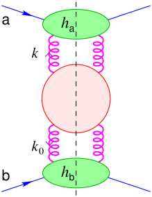
Figure 3.3: High energy factorization diagram for parton-parton scattering in dijet production.

Formally, we can write the colour and polarization averaged differential cross section

$${{\rm d}\sigma_{\text{\sf a}\text{\sf b}}\over{\rm d}{\boldsymbol{k}}\,{\rm d}{\boldsymbol{k}}_{0}}=\int{{\rm d}\omega\over 2\pi{\rm i}}\;\left({s\over s_{0}({\boldsymbol{k}},{\boldsymbol{k}}_{0})}\right)^{\omega}h_{\text{\sf a}}({\boldsymbol{k}})\,{\mathcal{G}}_{\omega}({\boldsymbol{k}},{\boldsymbol{k}}_{0})\,h_{\text{\sf b}}({\boldsymbol{k}}_{0})\;.$$ (3.9)

By assuming the GGF to be the resolvent of a NL$x$ kernel ${\mathcal{G}}_{\omega}=[\omega-{\mathcal{K}}]^{-1}$ and by expanding in $\bar{\alpha}_{\mathrm{s}}$ the impact factors and the kernel

$$h({\boldsymbol{k}}) =h^{(0)}({\boldsymbol{k}})+\bar{\alpha}_{\mathrm{s}}h^{(1)}({\boldsymbol{k}})+\cdots$$ (3.10)

$${\mathcal{K}}({\boldsymbol{k}},{\boldsymbol{k}}^{\prime}) =\bar{\alpha}_{\mathrm{s}}K^{(0)}({\boldsymbol{k}},{\boldsymbol{k}}^{\prime})+\bar{\alpha}_{\mathrm{s}}^{2}K^{(1)}({\boldsymbol{k}},{\boldsymbol{k}}^{\prime})+\cdots\;,$$ (3.11)

we obtain, after $\omega$-integration, the 1-loop expansion of (3.9)

$${{\rm d}\sigma_{\text{\sf a}\text{\sf b}}\over{\rm d}{\boldsymbol{k}}\,{\rm d}{\boldsymbol{k}}_{0}}=h_{\text{\sf a}}^{(0)}h_{\text{\sf b}}^{(0)}+\bar{\alpha}_{\mathrm{s}}\left[h_{\text{\sf a}}^{(0)}K^{(0)}h_{\text{\sf b}}^{(0)}\ln{s\over s_{0}}+h_{\text{\sf a}}^{(1)}h_{\text{\sf b}}^{(0)}+h_{\text{\sf a}}^{(0)}h_{\text{\sf b}}^{(1)}\right]+\cdots\;.$$ (3.12)

It is easy to recognize, in the second term of the above expansion, the leading $\ln s$ term whose coefficient provides the L$x$ BFKL kernel, whilst the constant (in $s$) ones yields the impact factor corrections. However, the ambiguity in the energy scale $s_{0}$ affects the definition of the impact factor correction, and a “scale fixing” prescription has to be introduced.

We define the impact factors by the following factorization procedure [26, 27]:

• subtract the leading term with a reference scale, consistently with the IR and collinear properties of the process;

• interpret the remaining constant at single-${\boldsymbol{k}}$ factorization level as the 1-loop correction $h^{(1)}$.

The definition of the impact factor correction $h^{(1)}$ can be accomplished by the 1-loop calculation of the differential cross section, which involves the known [29] particle-particle-reggeon (PPR) vertex at virtual level (the reggeon trajectory correction giving a L$x$ contribution) and require an accurate treatment of the squared matrix element for one particle production in the fragmentation regions of the incoming particles [26, 27].

Because of the UV singularities stemming from the loop integrals in the virtual correction diagrams, we adopt dimensional regularization in $D=4+2\varepsilon$ space-time dimensions. In this way we regularize at the same time the IR singularities when considering real and virtual emission separately. Definitions and details are deferred to App. B.

3.2.1 Quark impact factor

Let’s start by considering quark-quark scattering in which an additional gluon g of momentum $q$ is produced. According to the Sudakov parametrization

$$k_{1} =z_{1}p_{1}+\bar{z}_{1}p_{2}+{\boldsymbol{k}}_{1}\qquad({\boldsymbol{k}}_{1}=-{\boldsymbol{k}}) \bar{z}_{1} =-{{\boldsymbol{k}}_{1}^{2}\over(1-z_{1})s}\;,$$ (3.13a)

$$k_{2} =z_{2}p_{1}+\bar{z}_{2}p_{2}+{\boldsymbol{k}}_{2}\qquad({\boldsymbol{k}}_{2}={\boldsymbol{k}}_{0}) z_{2} =-{{\boldsymbol{k}}_{2}^{2}\over(1-\bar{z}_{2})s}\;,$$ (3.13b)

we define the “rapidity” of the gluon $y\,\raisebox{0.37pt}{:}=\ln(z_{1}\sqrt{s}/|{\boldsymbol{q}}|)$ which can assume the values $y\in[-Y,Y]$ where $Y\,\raisebox{0.37pt}{:}=\ln(\sqrt{s}/|{\boldsymbol{q}}|)$.

In the central region, corresponding to $|y|\ll Y$, the squared matrix element is correctly obtained by the amplitude

$${{\rm d}\sigma_{\text{\sf q}\text{\sf q}\to\text{\sf q}\text{\sf g}\text{\sf q}}^{(\text{L}x)}\over{\rm d}z_{1}\,{\rm d}{\boldsymbol{k}}_{1}{\rm d}{\boldsymbol{k}}_{2}}=h_{\text{\sf q}}^{(0)}({\boldsymbol{k}}_{1})\,{1\over z_{1}}\,{\bar{\alpha}_{\mathrm{s}}\over\pi_{\varepsilon}{\boldsymbol{q}}^{2}}\,h_{\text{\sf q}}^{(0)}({\boldsymbol{k}}_{2})\quad,\quad\pi_{\varepsilon}\,\raisebox{0.37pt}{:}=\pi^{1+\varepsilon}\Gamma(1-\varepsilon)\mu^{2\varepsilon}$$ (3.14)

which is nothing but Eq. (2.44) without reggeization of the gluon.

Outside the central region ($|y|\gg 1$), Eq. (3.14) does not hold at NL$x$ accuracy. The real emission amplitude, assuming the gluon in the a quark fragmentation region, can be computed by means of high energy factorization

$$\overline{|{\mathcal{M}}_{\text{\sf q}\text{\sf q}\to\text{\sf q}\text{\sf g}\text{\sf q}}|^{2}}={1\over N_{c}^{2}-1}g_{\varepsilon}^{2}C_{F}{1\over(k_{2}^{2})^{2}}\sum_{c,d,\lambda}|\overset{*}{\epsilon}{}_{(\lambda)}^{\mu}\,2p_{2}^{\nu}\,A_{\mu\nu}^{cd}|^{2}\;,$$ (3.15)

i.e., by coupling the fragmentation tensor $A_{\mu\nu}^{cd}$ of Fig. 3.4 to the b quark with an eikonal vertex, because of the strong ordering between the sub-energies $s_{1}\,\raisebox{0.37pt}{:}=(p^{\prime}_{1}+q)^{2}\ll s_{2}\,\raisebox{0.37pt}{:}=(q+p_{2}^{\prime})^{2}$.

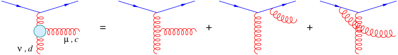
Figure 3.4: Quark-to-gluon fragmentation tensor $A_{\mu\nu}^{cd}$.

By using the three-body phase space at NL$x$ accuracy (B.4) we get

$$\frac{{\rm d}\sigma_{\text{\sf q}\text{\sf q}\to\text{\sf q}\text{\sf g}\text{\sf q}}^{(\text{NL}x)}}{{\rm d}z_{1}\,{\rm d}{\boldsymbol{k}}_{1}\,{\rm d}{\boldsymbol{k}}_{2}}=\; h_{\text{\sf q}}^{(0)}({\boldsymbol{k}}_{1})\,h_{\text{\sf q}}^{(0)}({\boldsymbol{k}}_{2})\,\frac{{\mathcal{P}}_{\text{\sf g}\text{\sf q}}(z_{1},\varepsilon)}{\pi_{\varepsilon}}\times$$

$$\times\left(\frac{C_{A}\alpha_{\mathrm{s}}}{\pi}\,\frac{(1-z_{1}){\boldsymbol{q}}\!\cdot\!({\boldsymbol{q}}-z_{1}{\boldsymbol{k}}_{2})}{{\boldsymbol{q}}^{2}\,({\boldsymbol{q}}-z_{1}{\boldsymbol{k}}_{2})^{2}}+\frac{C_{F}\alpha_{\mathrm{s}}}{\pi}\,\frac{z_{1}^{2}{\boldsymbol{k}}_{1}^{2}}{{\boldsymbol{q}}^{2}\,({\boldsymbol{q}}-z_{1}{\boldsymbol{k}}_{2})^{2}}\right)$$ (3.16)

where

$${\mathcal{P}}_{\text{\sf g}\text{\sf q}}(z,\varepsilon)=\frac{1}{2z}\left[1+(1-z)^{2}+\varepsilon z^{2}\right]$$ (3.17)

is related to the quark-to-gluon splitting function.

We can easily check that ${\rm d}\sigma_{\text{\sf q}\text{\sf q}\to\text{\sf q}\text{\sf g}\text{\sf q}}^{(\text{NL})}$ matches ${\rm d}\sigma^{(\text{L})}_{\text{\sf q}\text{\sf g}\text{\sf q}}$ (3.14) in the central region $z_{1}\ll 1$ — the $C_{F}$ term being suppressed by a factor $z_{1}^{2}$ — so that we can take it as the right differential cross section in the whole positive $q^{\mu}$ rapidity range

$$y>0\quad\iff\quad z_{1}>\sqrt{{\boldsymbol{q}}^{2}\over s}\;.$$ (3.18)

In the remaining half phase-space $y<0$ the cross section has the same expression provided we exchange ${\boldsymbol{k}}_{1}\leftrightarrow{\boldsymbol{k}}_{2}\;,\;z_{1}\leftrightarrow z_{2}$.

It is worth noting that the splitting function (3.17) is factored out in Eq. (3.16) even outside the collinear regions ${\boldsymbol{q}}^{2}\ll{\boldsymbol{k}}_{1}^{2}\simeq{\boldsymbol{k}}_{2}^{2}$ and ${\boldsymbol{k}}_{1}^{2}\ll{\boldsymbol{q}}^{2}\simeq{\boldsymbol{k}}_{2}^{2}$ thus suggesting a smooth extrapolation between collinear and Regge regions [30].

The cross section in Eq. (3.16) contains two colour factors which have a simple interpretation, depending on the collinear singularities involved. The $C_{F}$ term, with singularities at ${\boldsymbol{q}}^{2}=0$ ($({\boldsymbol{q}}-z_{1}{\boldsymbol{k}}_{2})^{2}=0$), comes from the Sudakov jet region, in which the emitted gluon is collinear to the incoming (outgoing) quark.

On the other hand, the $C_{A}$ term is not really singular at either ${\boldsymbol{q}}^{2}=0$ or $({\boldsymbol{q}}-z_{1}{\boldsymbol{k}}_{2})^{2}=0$, except for $z_{1}\simeq 0$, which correspond to the central region. It comes from the “coherent” region in which the gluon is emitted at angles which are large with respect to the $\widehat{\vec{p}_{1}\vec{p}_{1}{}^{\prime}}$ angle, and is thus sensitive to the total $\text{\sf q}\text{\sf q}^{\prime}$ charge $C_{A}$. This is the region we are interested in, which is relevant for the energy scale, because it tells us how the leading matrix element, valid in the central region, is cut-off in the fragmentation region.

We can simply realize the angular ordering phenomenon in the $C_{A}$ part of the real emission contribution to the cross section (3.16) upon azimuthal averaging in ${\boldsymbol{k}}_{1}$ at fixed ${\boldsymbol{q}}$, obtaining

$$\left\langle\frac{{\rm d}\sigma_{\text{\sf q}\text{\sf q}\to\text{\sf q}\text{\sf g}\text{\sf q}}}{{\rm d}z_{1}\,{\rm d}{\boldsymbol{k}}_{1}\,{\rm d}{\boldsymbol{k}}_{2}}\right\rangle=\;h_{\text{\sf q}}^{(0)}({\boldsymbol{k}}_{1})\,h_{\text{\sf q}}^{(0)}({\boldsymbol{k}}_{2})\,\frac{{\mathcal{P}}_{\text{\sf g}\text{\sf q}}(z_{1},\varepsilon)}{\pi_{\varepsilon}{\boldsymbol{q}}^{2}}\frac{C_{A}\alpha_{\mathrm{s}}}{\pi}\,\Theta(|{\boldsymbol{q}}|(1-z_{1})-|{\boldsymbol{k}}_{1}|z_{1})$$ (3.19)

The latter is the coherence effect prescription of Ref. [30] in which the polar angles of the emitted gluon and recoiling quark obey

$${|{\boldsymbol{q}}|\over z_{1}}>{|{\boldsymbol{k}}_{1}|\over 1-z_{1}}\quad\iff\quad\theta_{q}>\theta_{p_{1}^{\prime}}\;.$$ (3.20)

Roughly speaking, for ${\boldsymbol{q}}^{2}\gtrsim{\boldsymbol{k}}_{1}^{2}$ the half phase space $\sqrt{{\boldsymbol{q}}^{2}/s}<z_{1}<1$ is available in full, whilst, for ${\boldsymbol{k}}_{1}^{2}\ll{\boldsymbol{q}}^{2}$ it is dynamically restricted to $\sqrt{{\boldsymbol{q}}^{2}/s}<z_{1}<|{\boldsymbol{q}}|/(|{\boldsymbol{k}}_{1}|+|{\boldsymbol{q}}|)\simeq|{\boldsymbol{q}}|/|{\boldsymbol{k}}_{1}|$. With the parallel consideration in the other half phase space, the longitudinal integration of (3.19) provides the logarithmic factor

$$\int_{q/\sqrt{s}}^{1}{\rm d}z_{1}\;{\mathcal{P}}_{\text{\sf g}\text{\sf q}}(z_{1},\varepsilon)\Theta(|{\boldsymbol{q}}|(1-z_{1})-|{\boldsymbol{k}}_{1}|z_{1})+\{1\leftrightarrow 2\}\simeq\ln{s\over\operatorname{{\rm Max}}({\boldsymbol{q}},{\boldsymbol{k}}_{1})\operatorname{{\rm Max}}({\boldsymbol{q}},{\boldsymbol{k}}_{2})}$$ (3.21)

suggesting the natural scale of $s$ to be $s_{0}=s_{M}\,\raisebox{0.37pt}{:}=\operatorname{{\rm Max}}({\boldsymbol{q}},{\boldsymbol{k}}_{1})\operatorname{{\rm Max}}({\boldsymbol{q}},{\boldsymbol{k}}_{2})$ and hence the subtraction to be adopted in order to isolate the 1-loop impact factors.

More precisely, we define as leading real emission term of the differential cross section in the half phase space $y>0$ the quantity

$$h_{\text{\sf a}}^{(0)}({\boldsymbol{k}}_{1})\,h_{\text{\sf b}}^{(0)}({\boldsymbol{k}}_{2})\,{\Theta(|{\boldsymbol{q}}|-z_{1}|{\boldsymbol{k}}_{1}|)\over z_{1}}\,{\alpha_{\mathrm{s}}C_{A}\over\pi}{1\over\pi_{\varepsilon}{\boldsymbol{q}}^{2}}\qquad\big{(}z_{1}>\sqrt{{\boldsymbol{q}}^{2}\over s}\big{)}$$ (3.22)

which we subtract from Eq. (3.16) and interpret as the real emission contribution to the $\bar{\alpha}_{\mathrm{s}}h_{\text{\sf a}}^{(1)}({\boldsymbol{k}}_{1})h_{\text{\sf b}}^{(0)}({\boldsymbol{k}}_{2})$ term in the expansion (3.9). In this way we have fulfilled the first prescription for the definition of the impact factors, because the ($C_{A}$ part of the) subtracted term is finite in the ${\boldsymbol{q}}\to 0$ limit even for $z=0$ and therefore, according to the second prescription, after integration over all but one transverse variable, it defines an impact factor correction with the right collinear singularities. Explicitly, after subtracting (3.22) from (3.16), dropping the “lower” impact factor $h_{\text{\sf q}}^{(0)}({\boldsymbol{k}}_{2})$, and integrating over $z_{1}>\sqrt{{\boldsymbol{q}}^{2}/s}$ and ${\boldsymbol{k}}_{1}$ at fixed ${\boldsymbol{k}}_{2}$ we get

$$h_{\text{\sf q}}^{(1)}({\boldsymbol{k}}_{2})\Big{|}^{\text{real}}_{C_{A}} \simeq\int{\rm d}{\boldsymbol{k}}_{1}\;h_{\text{\sf q}}^{(0)}({\boldsymbol{k}}_{1}){1\over\pi_{\varepsilon}{\boldsymbol{q}}^{2}}$$

$$\quad\times\int_{0}^{1}{\rm d}z_{1}\;{\mathcal{P}}_{\text{\sf g}\text{\sf q}}(z_{1},\varepsilon){(1-z_{1}){\boldsymbol{q}}\!\cdot\!({\boldsymbol{q}}-z_{1}{\boldsymbol{k}}_{2})\over({\boldsymbol{q}}-z_{1}{\boldsymbol{k}}_{2})^{2}}-{\Theta(|{\boldsymbol{q}}|-z_{1}|{\boldsymbol{k}}_{1}|)\over z_{1}}$$

$$=\left(-{3\over 4\varepsilon}-2\psi^{\prime}(1)-{1\over 4}\right)\left({{\boldsymbol{k}}_{2}^{2}\over\mu^{2}}\right)^{\varepsilon}\,h_{\text{\sf q}}^{(0)}({\boldsymbol{k}}_{2})$$ (3.23a)

for the $$C_{A}$$ part of real emission and

$$h_{\text{\sf q}}^{(1)}({\boldsymbol{k}}_{2})\Big{|}^{\text{real}}_{C_{F}} \simeq{C_{F}\over C_{A}}\int{\rm d}{\boldsymbol{k}}_{1}\;h_{\text{\sf q}}^{(0)}({\boldsymbol{k}}_{1}){1\over\pi_{\varepsilon}{\boldsymbol{q}}^{2}}\int_{0}^{1}{\rm d}z_{1}\;{\mathcal{P}}_{\text{\sf g}\text{\sf q}}(z_{1},\varepsilon){z_{1}^{2}{\boldsymbol{k}}_{1}^{2}\over({\boldsymbol{q}}-z_{1}{\boldsymbol{k}}_{2})^{2}}$$

$$=\bar{\alpha}_{\mathrm{s}}{C_{F}\over C_{A}}\left({1\over\varepsilon^{2}}-{3\over 2\varepsilon}+4-\psi^{\prime}(1)\right)\left({{\boldsymbol{k}}_{2}^{2}\over\mu^{2}}\right)^{\varepsilon}\,h_{\text{\sf q}}^{(0)}({\boldsymbol{k}}_{2})$$ (3.23b)

for the $C_{F}$ part. Note that the lower bound of the $z$-integrations has been pushed down to zero since, in the $s\to\infty$ limit, the error is negligible. The real emission correction to the lower impact factor are provided by the left half phase space contribution $y<0$.

The ${1/\varepsilon}$ pole in Eq. (3.23b) comes as no surprise, because it corresponds to the collinear divergence at ${\boldsymbol{k}}_{1}^{2}=0$ due to $\text{\sf q}\to\text{\sf g}$ transition of the initial massless quark. This is what we intended with “consistent with the collinear properties”. A different subtraction could have produced a double pole in $\varepsilon$ which is not consistent with the collinear singularity.

As far as the $C_{F}$ term is concerned, we do have a double pole in $\varepsilon$. This is not a problem, because, as we shall see soon, the whole $C_{F}$ contribution is cancelled by virtual corrections.

The correction to the cross section due to virtual emission, including subleading effects, for general parton-parton scattering, can be extracted from the amplitude of Ref. [29]

$${\mathcal{M}}^{(0+1,\text{NL})}_{\text{\sf a}\text{\sf b}\to\text{\sf a}\text{\sf b}}=-i\,2s\,\Gamma_{aa^{\prime}}^{c}\Big{(}1+\bar{\alpha}_{\mathrm{s}}\Pi^{(+)}_{\text{\sf a}\text{\sf a}}\Big{)}\frac{1}{t}\left[1+\Omega^{(0)}(-t)\ln\frac{s}{-t}\right]\Big{(}1+\bar{\alpha}_{\mathrm{s}}\Pi^{(+)}_{\text{\sf b}\text{\sf b}}\Big{)}\Gamma_{bb^{\prime}}^{c}$$ (3.24)

where $\Gamma_{aa^{\prime}}^{c}$ is the particle-gluon vertex of Eqs. (2.30). The $\ln s$ term provides the 1-loop Regge gluon trajectory (Eq. (2.32b)) and the finite terms $\Pi^{(+)}({\boldsymbol{k}}^{2})$ define the PPR vertex correction in the helicity conserving channel.

In the quark case

$$\Pi^{(+)}_{\text{\sf q}\text{\sf q}}={1\over 2}\left[-\frac{11}{12\varepsilon}+\left(\frac{85}{36}+\frac{\pi^{2}}{4}\right)+\frac{N_{\!f}}{N_{c}}\left(\frac{1}{6\varepsilon}-\frac{5}{18}\right)-\frac{C_{F}}{N_{c}}\left(\frac{1}{\varepsilon^{2}}-\frac{3}{2\varepsilon}+4-\psi^{\prime}(1)\right)\right]\!\!\left({{\boldsymbol{k}}^{2}\over\mu^{2}}\right)^{\!\varepsilon}\,.$$ (3.25)

The virtual contribution to the 1-loop cross section is given by the interference between (3.24) and the Born amplitude (2.29) together with the two-body phase space measure (B.3) yielding

$${{\rm d}\sigma^{(1)}_{\text{\sf q}\text{\sf q}\to\text{\sf q}\text{\sf q}}\over{\rm d}{\boldsymbol{k}}_{1}\,{\rm d}{\boldsymbol{k}}_{2}}=\bar{\alpha}_{\mathrm{s}}h_{\text{\sf q}}^{(0)}({\boldsymbol{k}}_{1})h_{\text{\sf q}}^{(0)}({\boldsymbol{k}}_{2})\,\left[2\Omega^{(0)}({\boldsymbol{k}}_{1}^{2})\ln{s\over{\boldsymbol{k}}_{1}^{2}}+4\Pi_{\text{\sf q}\text{\sf q}}^{(+)}({\boldsymbol{k}}_{1}^{2})\right]\delta({\boldsymbol{k}}_{1}-{\boldsymbol{k}}_{2})\;.$$ (3.26)

The first term in the above equation is the virtual part of the leading BFKL kernel. The second one provides the virtual contribution to the last two terms in Eq. (3.9), so that

$$h_{\text{\sf q}}^{(1)}({\boldsymbol{k}}_{2})\Big{|}^{\text{virt}}_{C_{A}} =\left[-\frac{11}{12\varepsilon}+\left(\frac{85}{36}+\frac{\pi^{2}}{4}\right)+\frac{N_{\!f}}{N_{c}}\left(\frac{1}{6\varepsilon}-\frac{5}{18}\right)\right]\left({{\boldsymbol{k}}_{2}^{2}\over\mu^{2}}\right)^{\varepsilon}h_{\text{\sf q}}^{(0)}({\boldsymbol{k}}_{2})$$ (3.27a)

$$h_{\text{\sf q}}^{(1)}({\boldsymbol{k}}_{2})\Big{|}^{\text{virt}}_{C_{F}} ={C_{F}\over C_{A}}\left(-{1\over\varepsilon^{2}}+{3\over 2\varepsilon}-4+\psi^{\prime}(1)\right)\left({{\boldsymbol{k}}_{2}^{2}\over\mu^{2}}\right)^{\varepsilon}h_{\text{\sf q}}^{(0)}({\boldsymbol{k}}_{2})$$ (3.27b)

When adding the RHS of Eqs. (3.23) and (3.27), one can immediately see the cancellation of the $C_{F}$ terms and obtain the complete 1-loop impact factor correction [26]

$$h_{\text{\sf q}}^{(1)}({\boldsymbol{k}})=\left[-{1\over\varepsilon}\left(\frac{11N_{c}-2N_{\!f}}{12N_{c}}\right)-{1\over 2\varepsilon}\left(\frac{3}{2}-\frac{1}{2}\varepsilon\right)+{1\over 2}\left(\frac{67}{18}-\frac{\pi^{2}}{6}-\frac{5N_{\!f}}{9N_{c}}\right)\right]\left({{\boldsymbol{k}}^{2}\over\mu^{2}}\right)^{\varepsilon}h_{\text{\sf q}}^{(0)}({\boldsymbol{k}})$$ (3.28)

3.2.2 Gluon impact factor

We consider now gluon-gluon scattering. In this case we have to distinguish two different final states for three-particle production. In addition to the gluon $\text{\sf g}^{\prime}$ there may be:

• two gluons;

• a quark-antiquark pair.

$\text{\sf g}\text{\sf g}\to\text{\sf g}\text{\sf g}\text{\sf g}$

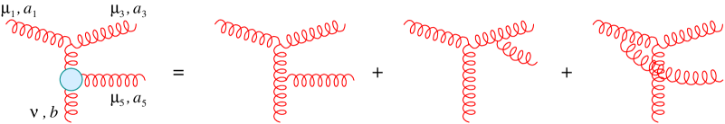
Figure 3.5: Gluon-to-gluon fragmentation tensor $A_{\mu_{1}\mu_{3}\mu_{5}\nu}^{a_{1}a_{3}a_{5}b}$.

Assume that the additional gluon is emitted in the gluon a fragmentation region. By using again high energy factorization, the scattering amplitude in the Feynman gauge is given by

$${\mathcal{M}}^{(1)}_{\text{\sf g}\text{\sf g}\to\text{\sf g}\text{\sf g}\text{\sf g}}=\epsilon_{1}^{\mu_{1}}\,\overset{*}{\epsilon}\,{}_{3}^{\mu_{3}}\,\overset{*}{\epsilon}\,{}_{5}^{\mu_{5}}\;A_{\mu_{1}\mu_{3}\mu_{5}\,\nu}^{a_{1}a_{3}a_{5}\,b}\,\frac{1}{k_{2}^{2}}\;g\,2p_{2}^{\nu}\,\overset{b}{T}{}_{\text{\sf b}}\,\delta_{\lambda_{4}\lambda_{2}}$$ (3.29)

where the amplitude $A$, corresponding to the diagrams of Fig. 3.5 was found in Ref. [31] to be

$$A_{\mu_{1}\mu_{3}\mu_{5}\,\nu}^{a_{1}a_{3}a_{5}\,b}\,2p_{2}^{\nu} =4g^{2}\,g_{\mu_{1}\mu_{3}}\Big{[}{\rm f}^{a_{1}a_{5}e}{\rm f}^{ea_{3}b}D_{\mu_{5}}(-p_{1},p_{3},p_{5})+{\rm f}^{a_{3}a_{5}e}{\rm f}^{ea_{1}b}D_{\mu_{5}}(p_{3},-p_{1},p_{5})\Big{]}+$$

$$\qquad+\,\begin{picture}(23.0,9.0)(0.0,5.0)\put(0.0,4.5){$\Bigg{(}$}\put(19.0,4.5){$\Bigg{)}$} \put(4.0,10.0){$p_{3}\leftrightarrow p_{5}$} \put(3.7,5.0){$\mu_{3}\leftrightarrow\mu_{5}$} \put(4.0,0.0){$a_{3}\leftrightarrow a_{5}$} \end{picture}+\,\begin{picture}(23.0,9.0)(0.0,5.0)\put(0.0,4.5){$\Bigg{(}$}\put(21.0,4.5){$\Bigg{)}$} \put(3.0,10.0){$-p_{1}\leftrightarrow p_{5}$} \put(6.0,5.0){$\mu_{1}\leftrightarrow\mu_{5}$} \put(6.3,0.0){$a_{1}\leftrightarrow a_{5}$} \end{picture}\quad,$$ (3.30)

where the current

$$D^{\mu}(x,y,z)=\frac{1}{x\!\cdot\!y}\left[\left(y\!\cdot\!z-p_{2}\!\cdot\!p_{4}\,\frac{p_{2}\!\cdot\!y}{p_{2}\!\cdot\!z}\right)p_{2}^{\mu}+\frac{p_{2}\!\cdot\!y}{x\!\cdot\!z}(y\!\cdot\!z-p_{2}\!\cdot\!p_{4})x^{\mu}+(x\!\cdot\!p_{2})y^{\mu}\right]$$ (3.31)

is a function of the momenta $x^{\alpha},y^{\alpha},z^{\alpha}$, with $x\!\cdot\!y=x^{\alpha}y_{\alpha}$.

The squared helicity amplitudes corresponding to Eq. (3.30) were given in Ref. [32]. Since we work in $D=4+2\varepsilon$ dimensions, we perform explicitly the polarization sum on Eq. (3.29). The averaged squared matrix element that we obtain is actually independent of the space-time dimensionality (i.e. $\varepsilon$-independent) so that we finally get

$$\frac{{\rm d}\sigma_{\text{\sf g}\text{\sf g}\text{\sf g}}}{{\rm d}z_{1}\,{\rm d}{\boldsymbol{k}}_{1}\,{\rm d}{\boldsymbol{k}}_{2}}=\; h_{\text{\sf g}}^{(0)}({\boldsymbol{k}}_{1})\,h_{\text{\sf b}}^{(0)}({\boldsymbol{k}}_{2})\,\frac{{\mathcal{P}}_{\text{\sf g}\text{\sf g}}(z_{1})}{\pi_{\varepsilon}}\times$$

$$\times\frac{C_{A}\alpha_{\mathrm{s}}}{\pi}\,\frac{z_{1}^{2}{\boldsymbol{k}}_{1}^{2}+(1-z_{1})^{2}{\boldsymbol{q}}^{2}+z_{1}(1-z_{1}){\boldsymbol{k}}_{1}\!\cdot\!{\boldsymbol{q}}}{{\boldsymbol{q}}^{2}\;(z_{1}{\boldsymbol{k}}_{1}+(1-z_{1}){\boldsymbol{q}})^{2}}\;.$$ (3.32)

This expression explicitly exhibits the symmetry in the exchange $-{\boldsymbol{k}}_{1}\leftrightarrow{\boldsymbol{q}}\;;\;z_{1}\leftrightarrow 1-z_{1}$ due to the identity of the gluons emitted in the fragmentation region of gluon a, but will be used for the softer gluon only $(z_{1}<\frac{1}{2})$, in order to avoid double counting.

The function

$${\mathcal{P}}_{\text{\sf g}\text{\sf g}}(z_{1})={\mathcal{P}}_{\text{\sf g}\text{\sf g}}(1-z_{1})=\frac{1+z_{1}^{4}+(1-z_{1})^{4}}{2z_{1}(1-z_{1})}$$ (3.33)

is related to the gluon to gluon splitting function, and is factored out in Eq. (3.2.2) in the whole fragmentation region, as for quark scattering. In this case also the cross section matches the leading expression (3.14) in the central region $z_{1}\ll 1$, and thus is taken to be valid in the half phase space (3.18) in which two of the three gluons have positive rapidity.

$\text{\sf g}\text{\sf g}\to\text{\sf q}\bar{\text{\sf q}}\text{\sf g}$

The main contribution to the cross section from this kind of final states is reached when the fermion pair belongs to the same fragmentation vertex, as in Fig. 3.6a. Other graphs like Fig. 3.6b are suppressed by a factor $|t|/s$ because of fermionic exchange.

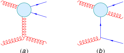
Figure 3.6: Quark-antiquark emission amplitudes: (a) The pair is emitted in the fragmentation region of the upper incoming gluon; (b) This kind of diagram is suppressed by a factor $|t|/s$.

Assuming $\text{\sf q}\bar{\text{\sf q}}$ being emitted in the fragmentation region of gluon a, and labelling q with “3” and $\bar{\text{\sf q}}$ with “5” ($p_{5}=q$), the corresponding amplitude is

$${\mathcal{M}}_{\text{\sf q}\overline{\text{\sf q}}\text{\sf g}}=\epsilon^{\mu}\,\overline{u}_{3}B_{\mu\nu}^{ab}v_{5}\,\frac{1}{k_{2}^{2}}\;g\,2p_{2}^{\mu}\,\overset{b}{T}{}_{\text{\sf q}}\,\delta_{\lambda_{4}\lambda_{2}}$$ (3.34)

where $B_{\mu\nu}^{ab}$ is the sum of the diagrams depicted in Fig. 3.7.

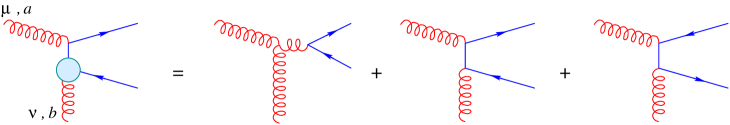
Figure 3.7: Gluon to quark fragmentation tensor $B_{\mu\nu}^{ab}$.

This calculation is very similar to the $\text{\sf q}\text{\sf q}\to\text{\sf q}\text{\sf g}\text{\sf q}$ cross section, and yields

$$\frac{{\rm d}\sigma_{\text{\sf q}\bar{\text{\sf q}}\text{\sf g}}}{{\rm d}z_{1}\,{\rm d}{\boldsymbol{k}}_{1}\,{\rm d}{\boldsymbol{k}}_{2}} =N_{\!f}\,h_{\text{\sf g}}^{(0)}({\boldsymbol{k}}_{2})\,\frac{\alpha_{\mathrm{s}}N_{\varepsilon}}{{\boldsymbol{k}}_{1}^{2}\mu^{2\varepsilon}}\,\frac{{\mathcal{P}}_{\text{\sf q}\text{\sf g}}(z_{1},\varepsilon)}{2\pi_{\varepsilon}}$$ (3.35)

$$\quad\times\left[\frac{C_{A}\alpha_{\mathrm{s}}}{\pi}\,\frac{-z_{1}(1-z_{1}){\boldsymbol{k}}_{1}\!\cdot\!{\boldsymbol{q}}}{{\boldsymbol{q}}^{2}\,(z_{1}{\boldsymbol{k}}_{1}+(1-z_{1}){\boldsymbol{q}})^{2}}+\frac{C_{F}\alpha_{\mathrm{s}}}{\pi}\,\frac{1}{{\boldsymbol{q}}^{2}}\right]$$

in which the function

$${\mathcal{P}}_{\text{\sf q}\text{\sf g}}(z_{1},\varepsilon)=1-\frac{2z_{1}(1-z_{1})}{1+\varepsilon}\quad,$$ (3.36)

related to the gluon to quark splitting function, is regular in $z_{1}\in[0,1]$. Hence these final states do not produce any $\ln s$ term, and need no subtraction.

The virtual correction to the amplitude, including NL$x$ effects, is given by an expression analogue to Eq. (3.24) where $\Pi^{(+)}_{\text{\sf a}\text{\sf a}}({\boldsymbol{k}}^{2})$ is replaced by the gluon-gluon-reggeon vertex correction [29] in the helicity conserving channel

$$\Pi^{(+)}_{\text{\sf g}\text{\sf g}}={1\over 2}\left[-\frac{1}{\varepsilon^{2}}+\frac{11}{12\varepsilon}-\left(\frac{67}{36}-\frac{\pi^{2}}{4}+\psi^{\prime}(1)\right)-\frac{N_{\!f}}{N_{c}}\left(\frac{1}{6\varepsilon}-\frac{5}{18}-\psi^{\prime}(1)\right)\right]\left({{\boldsymbol{k}}^{2}\over\mu^{2}}\right)^{\varepsilon}\;.$$ (3.37)

Now, with the result of experience of Sec. 3.2.1, we can obtain the gluon impact factor in a more direct way: let’s introduce the effective fragmentation vertex $F_{\text{\sf a}}(z_{1},{\boldsymbol{k}}_{1},{\boldsymbol{q}})$ of the incoming particle a defined in such a way that the 1-loop differential high energy cross section for ab scattering with possible emission of a new particle c with positive rapidity with respect to a is given by $F_{\text{\sf a}}$ times the exchanged Regge-gluon propagator and the full impact factor of particle b. In practice the effective fragmentation vertex represents the cross section of a with a Regge-gluon, including PPR virtual corrections and one-particle emission in NL$x$ approximation, as in Fig. 3.8.

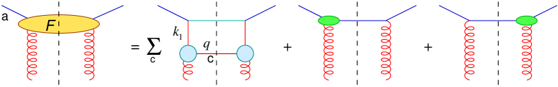
Figure 3.8: Effective parton Regge-gluon fragmentation vertex $F_{\text{\sf a}}$. In the RHS the circular blobs denotes the fragmentation tensors of Figs. 3.4, 3.5 and 3.7; the elliptic blobs corresponds to the PPR vertices $\Pi^{(+)}$.

In order to extract the 1-loop correction to the impact factor, we have to eliminate the $\ln s$ term by subtracting the leading fragmentation vertex — i.e., Eq. (3.22) without the second impact factor — containing the $1/z_{1}$ singularity coming from the splitting functions ${\mathcal{P}}_{\text{\sf g}\text{\sf a}}$:

$$\bar{\alpha}_{\mathrm{s}}h_{\text{\sf a}}^{(1)}({\boldsymbol{k}}_{2})=\int{\rm d}{\boldsymbol{k}}_{1}\int_{0}^{1}{\rm d}z_{1}\;F_{\text{\sf a}}(z_{1},{\boldsymbol{k}}_{1},{\boldsymbol{q}})-\bar{\alpha}_{\mathrm{s}}h_{\text{\sf a}}^{(0)}({\boldsymbol{k}}_{1})\,{\Theta(q-z_{1}k_{1})\over z_{1}}\,\frac{1}{\pi_{\varepsilon}{\boldsymbol{q}}^{2}}$$ (3.38)

From Eqs. (3.2.2), (3.35) and (3.37), we get the gluon fragmentation vertex

$$F_{\text{\sf g}} (z_{1},{\boldsymbol{k}}_{1},{\boldsymbol{q}})=h_{\text{\sf g}}^{(0)}({\boldsymbol{k}}_{1})\bigg{\{}\delta({\boldsymbol{q}})\delta(1-z_{1})\bar{\alpha}_{\mathrm{s}}2\Pi_{\text{\sf g}\text{\sf g}}^{(+)}({\boldsymbol{k}}_{1}^{2})$$ (3.39)

$$+N_{\!f}\frac{\alpha_{\mathrm{s}}}{\pi}\,\frac{{\mathcal{P}}_{\text{\sf q}\text{\sf g}}(z_{1},\varepsilon)}{2\pi_{\varepsilon}}\left[\frac{-z_{1}(1-z_{1}){\boldsymbol{k}}_{1}\!\cdot\!{\boldsymbol{q}}}{{\boldsymbol{q}}^{2}\,(z_{1}{\boldsymbol{k}}_{1}+(1-z_{1}){\boldsymbol{q}})^{2}}+\frac{C_{F}}{C_{A}}\,\frac{1}{{\boldsymbol{q}}^{2}}\right]$$

$$+\frac{\bar{\alpha}_{\mathrm{s}}}{\pi_{\varepsilon}}\,\Theta(\frac{1}{2}-z_{1}){\mathcal{P}}_{\text{\sf g}\text{\sf g}}(z_{1})\,\frac{z_{1}^{2}{\boldsymbol{k}}_{1}^{2}+(1-z_{1})^{2}{\boldsymbol{q}}^{2}+z_{1}(1-z_{1}){\boldsymbol{k}}_{1}\!\cdot\!{\boldsymbol{q}}}{{\boldsymbol{q}}^{2}\;(z_{1}{\boldsymbol{k}}_{1}+(1-z_{1})){\boldsymbol{q}}^{2}}\bigg{\}}\;.$$ (3.40)

Having identified $z_{1}$ as the momentum fraction of the softer gluon in $\text{\sf g}\text{\sf g}\to\text{\sf g}\text{\sf g}\text{\sf g}$ scattering, to avoid double counting due to final gluons identity, we restrict the naive half phase space to $z_{1}\in[\frac{q}{\sqrt{s}},\frac{1}{2}]$. In so doing, the 1-loop correction to the gluon impact factor is given by [27]

$$h_{\text{\sf g}}^{(1)}({\boldsymbol{k}}) =\left[-{1\over\varepsilon}\left(\frac{11N_{c}-2N_{\!f}}{12N_{c}}\right)+{1\over 2N_{c}}{1\over\varepsilon}\left(-{11N_{c}+(2+\varepsilon)N_{\!f}\over 6}\right)\right.$$ (3.41)

$$\quad\left.+{1\over 2N_{c}}{C_{F}\over C_{A}}{2N_{\!f}T_{R}\over\varepsilon}\left(\frac{2}{3}+\frac{1}{3}\varepsilon\right)+{1\over 2}\left(\frac{67}{18}-\frac{\pi^{2}}{6}-\frac{5N_{\!f}}{9N_{c}}\right)\right]\left({{\boldsymbol{k}}^{2}\over\mu^{2}}\right)^{\varepsilon}h_{\text{\sf g}}^{(0)}({\boldsymbol{k}})\;.$$

3.2.3 Colourless impact factors

It is possible to define impact factors for colourless sources — as in double-DIS processes — in a way analogous to the one adopted for partons. In this case, there is an additional dependence on the $\omega$ variable and on the external hard scale(s) so that, at leading level, the impact factors

$$h_{\text{\sf a}}^{(0)}=h_{\text{\sf a},\omega}^{(0)}(Q_{1},{\boldsymbol{k}}_{1})=\frac{1}{Q_{1}^{2}}\,f^{\text{\sf a}}_{\omega}\left(\frac{Q_{1}^{2}}{{\boldsymbol{k}}_{1}^{2}}\right)$$ (3.42)

yield a nontrivial ${\boldsymbol{k}}_{1}$-dependence, which has been explicitly computed in several processes [33]. In Eq. (3.42) the function $f_{\text{\sf a}}$ has the role of setting $k_{1}$ of order $Q_{1}$ in the total cross section, and has no ${\boldsymbol{k}}_{1}^{2}=0$ singularity at all, because there is no initial colour charge.

Therefore, by translating angular ordering into the $\omega$-space threshold factor $({\boldsymbol{q}}/{\boldsymbol{k}}_{1})^{\omega}$, the analogue of Eq. (3.38) becomes

$$\bar{\alpha}_{\mathrm{s}}h_{\text{\sf a},\omega}^{(1)}(Q_{1},{\boldsymbol{k}}_{2}) =\!\int\!\!{\rm d}{\boldsymbol{k}}_{1}\!\int_{0}^{1}\!\!{\rm d}z_{1}\,F_{\text{\sf a},\omega}(Q_{1},z_{1},{\boldsymbol{k}}_{1},{\boldsymbol{q}})-\bar{\alpha}_{\mathrm{s}}h_{\text{\sf a},\omega}^{(0)}(Q_{1},{\boldsymbol{k}}_{1})\,\frac{1}{\omega\pi_{\varepsilon}{\boldsymbol{q}}^{2}}\left(\frac{{\boldsymbol{q}}}{{\boldsymbol{k}}_{1}}\right)^{\!\omega\,\Theta(|{\boldsymbol{k}}_{1}|-|{\boldsymbol{q}}|)}.$$ (3.43)

In this case, no ${\boldsymbol{q}}=0$ nor ${\boldsymbol{k}}_{1}=0$ singularities are expected in $F_{\text{\sf a}}$, so that it is again important that the leading term be subtracted out with the angular ordering constraint.

We thus conclude that the definition of the impact factors in Eqs. (3.38) and (3.43), defines a self-consistent ${\boldsymbol{k}}$-factorization scheme of Eq. (3.9) for both coloured and colourless sources.

3.3 Collinear factorization and finite parts

We want now to analyze the structure of the quark and gluon impact factors derived in Secs. (3.2.1) and (3.2.2). The explicit expressions reported in Eqs. (3.28) and (3.41) show the presence of

• a $\beta$-function coefficient $\displaystyle{\frac{\pi}{N_{c}}\,b_{0}=\frac{11N_{c}-2N_{\!f}}{12N_{c}}}$;

• the finite part $\tilde{P}_{\text{\sf b}\text{\sf a}}(\omega=0)$ in the $\omega$ expansion of the Mellin transform of the $\sf a\to b=q,g$ splitting functions for the incoming parton a under consideration, as depicted in Tab. (3.1);

• a common and $\varepsilon$-finite factor $\displaystyle{\frac{{\mathcal{K}}}{N_{c}}\,\raisebox{0.37pt}{:}=\left(\frac{67}{18}-\frac{\pi^{2}}{6}-\frac{5N_{\!f}}{9N_{c}}\right)}$.

c $\leftarrow$ a	$P_{\text{\sf c}\text{\sf a}}(z,\varepsilon)$	$\int_{0}^{1}z^{\omega}P_{\text{\sf c}\text{\sf a}}(z,\varepsilon)\,{\rm d}z$
q  q	$\displaystyle{C_{F}\left[\left(\frac{1+z^{2}}{1-z}\right)_{+}-\varepsilon(1-z)+\frac{\varepsilon}{2}\,\delta(1-z)\right]}$	$0+{\mathcal{O}}(\omega)$
g  q	$\displaystyle{C_{F}\left[\frac{1+(1-z)^{2}}{z}+\varepsilon z\right]}$	$\displaystyle{\frac{2C_{F}}{\omega}-C_{F}\left(\frac{3}{2}-\frac{1}{2}\varepsilon\right)+{\mathcal{O}}(\omega)}$
q  g	$\displaystyle{T_{R}\left[1-\frac{2z(1-z)}{1+\varepsilon}\right]}$	$\displaystyle{T_{R}\left(\frac{2}{3}+\frac{1}{3}\,\varepsilon\right)+{\mathcal{O}}(\omega)}$
g  g	$\displaystyle{2N_{c}\left[\frac{1-z}{z}+\frac{z}{(1-z)_{+}}+z(1-z)\right]+\frac{11N_{c}-2N_{\!f}}{6}\delta(1-z)}$	$\displaystyle{\frac{2N_{c}}{\omega}-\frac{11N_{c}+(2+\varepsilon)N_{\!f}}{6}+{\mathcal{O}}(\omega)}$

Table 3.1: Partonic splitting functions and Mellin transforms in $\omega$-space.

This suggests writing the complete one-loop impact factors $h_{\text{\sf a}}({\boldsymbol{k}})=h^{(0)}_{\text{\sf a}}({\boldsymbol{k}})+\bar{\alpha}_{\mathrm{s}}h^{(1)}_{\text{\sf a}}({\boldsymbol{k}})$ for both $\text{\sf a}=\text{\sf q},\text{\sf g}$ in the following manner:

$$h_{\text{\sf a}}({\boldsymbol{k}}) =h^{(0)}_{\text{\sf a}}({\boldsymbol{k}})+\bar{\alpha}_{\mathrm{s}}\left[-{\pi\over N_{c}}{b_{0}\over\varepsilon}h^{(0)}_{\text{\sf a}}({\boldsymbol{k}})+{1\over 2N_{c}}\sum_{\text{\sf c}}h_{\text{\sf c}}^{(0)}({\boldsymbol{k}}){\tilde{P}_{\text{\sf c}\text{\sf a}}\over\varepsilon}+{1\over 2N_{c}}h^{(0)}_{\text{\sf a}}({\boldsymbol{k}})\,{\mathcal{K}}\right]\left({{\boldsymbol{k}}^{2}\over\mu^{2}}\right)^{\varepsilon}$$ (3.44)

$$=\left[1-{b_{0}\over\varepsilon}\alpha_{\mathrm{s}}\left({{\boldsymbol{k}}^{2}\over\mu^{2}}\right)^{\varepsilon}\right]\left\{h^{(0)}_{\text{\sf a}}({\boldsymbol{k}})+{\alpha_{\mathrm{s}}\over 2\pi}\left[h^{(0)}_{\text{\sf a}}({\boldsymbol{k}})\,{\mathcal{K}}+\sum_{\text{\sf c}}h_{\text{\sf c}}^{(0)}({\boldsymbol{k}}){\tilde{P}_{\text{\sf c}\text{\sf a}}\over\varepsilon}\left({{\boldsymbol{k}}^{2}\over\mu^{2}}\right)^{\varepsilon}\right]\right\}\;.$$

The factor in front of the last expression provides the renormalization of the coupling constant, and by introducing the one-loop running coupling

$$\alpha_{\mathrm{s}}({\boldsymbol{k}}^{2})=\alpha_{\mathrm{s}}\left[1-b_{0}\,\frac{\alpha_{\mathrm{s}}}{\varepsilon}\left(\frac{{\boldsymbol{k}}^{2}}{\mu^{2}}\right)^{\varepsilon}\right]\quad,$$ (3.45)

it can be incorporated in $h_{\text{\sf a}}^{(0)}$ itself.

Therefore, the impact factors in Eq. (3.44) assume the form

$$h_{\text{\sf a}}({\boldsymbol{k}}^{2})=h_{\text{\sf a}}^{(0)}({\boldsymbol{k}};\alpha_{\mathrm{s}}({\boldsymbol{k}}^{2}))\left(1+\frac{\alpha_{\mathrm{s}}}{2\pi}\,{\mathcal{K}}\right)+\frac{\alpha_{\mathrm{s}}}{2\pi}\left[h_{\text{\sf q}}^{(0)}\frac{\tilde{P}_{\text{\sf q}\text{\sf a}}}{\varepsilon}+h_{\text{\sf g}}^{(0)}\frac{\tilde{P}_{\text{\sf g}\text{\sf a}}}{\varepsilon}\right]\left(\frac{{\boldsymbol{k}}^{2}}{\mu^{2}}\right)^{\varepsilon}$$ (3.46)

and thus satisfy the DGLAP equations with splitting functions $\tilde{P}_{\text{\sf c}\text{\sf a}}(\omega=0)$.

After factorization of the collinear singularities contained in the latter, the only finite renormalization is the one implied by the factor $\displaystyle{\left(1+\frac{\alpha_{\mathrm{s}}}{2\pi}\,{\mathcal{K}}\right)}$, which is universal, i.e. independent of the parton type.

Several comments are in order. First, the collinear singularities in $h_{\text{\sf a}}$ do not contain the $\sim 1/\omega$ terms of the splitting functions, which have been subtracted out in the leading term. In this context, we remark the difference between the double-${\boldsymbol{k}}$ cross section defined here through ${\boldsymbol{k}}$-factorization, and the double-mini-jet inclusive cross section defined by Mueller and Navelet [28].

In the latter case the cross section is inclusive over all fragmentation products of the incoming partons which are not identified, and measures the gluonic ${\boldsymbol{k}}$’s only because of collinear strong ordering. Therefore, it factorizes the gluon distribution density in the parton, rather than the impact factor, with all its collinear singularities included and, furthermore, can be applied only at leading $\ln s$ level because of strong ordering.

On the other hand, in our case the definition of the ${\boldsymbol{k}}$-dependent cross section is more precise, but can be done theoretically rather than experimentally, because one needs not only to identify all fragmentation products, but also to subtract out the central region tail — which appears to be hard to do experimentally. Because of this difference, the collinear singularities to be factored out are different in the two cases.

As a second point we remark that a universal renormalization, with the same ${\mathcal{K}}$ coefficient, holds also for the soft part of the one-loop time-like splitting functions [34]. This part has a next-to-leading $1/(1-z_{1})$ singularity, the leading one having a logarithmic factor, and is therefore analogous to the impact factor, which corresponds to the NL$x$ constant piece in the high-energy limit.

The above analogy is perhaps a hint [35] to explain the universality found here. However our result does not seem to follow in a clearcut way, because of the difference between collinear and high-energy factorization pointed out before.

3.4 Which of the energy-scales?

The problem of choosing the energy scale $s_{0}({\boldsymbol{k}},{\boldsymbol{k}}_{0})$ is not concerned only with the collinear behaviour of the impact factors, but also with the validity of the NL$x$ factorization formula (3.9) to all orders in $\alpha_{\mathrm{s}}$ and with the definition of the GGF.

One could ask whether Eq. (3.9) really holds to all orders when $s_{0}=s_{M}$ is adopted as energy-scale. If not, is it possible to properly define the impact factors and the GGF in such a way that, for a different choice of $s_{0}$ the factorization formula is valid?

These questions naturally arise when noticing that the scale $s_{M}$ of Eq. (3.21) has the defect of not being factorized in its ${\boldsymbol{k}}_{1},{\boldsymbol{k}}_{2}$ dependence. This fact is argued to contradict multi-Regge factorization of production amplitudes [36], which implies short-range correlations of the ${\boldsymbol{k}}$’s. Furthermore, the use of $O(2,1)$ variables [37] implies that Regge behaviour in the energy $s$ should involve the boost (in the following $k_{i}\,\raisebox{0.37pt}{:}=|{\boldsymbol{k}}_{i}|$, $q\,\raisebox{0.37pt}{:}=|{\boldsymbol{q}}|$)

$$\cosh(\zeta)=\frac{s}{2k_{1}k_{2}}\quad,$$ (3.47)

thus suggesting the choice $s_{0}=k_{1}k_{2}$.

We are going to show that, if the factorized scale $s_{0}=k_{1}k_{2}$ is chosen, then at 1-loop level the definition of the GGF has to be modified with respect to Eq. (2.53) by introducing two $\omega$-independent additional kernel.

The 1-loop cross section restricted to half the phase space $z_{1}<q/\sqrt{s}$ can be represented, apart from the b impact factor and the Regge-gluon trajectory, by the effective fragmentation vertex

$$\int_{q/\sqrt{s}}^{1}{\rm d}z_{1}\;F_{\text{\sf a}}(z_{1},{\boldsymbol{k}}_{1},{\boldsymbol{q}}) =h_{\text{\sf a}}^{(0)}({\boldsymbol{k}}_{1}){\bar{\alpha}_{\mathrm{s}}\over\pi_{\varepsilon}{\boldsymbol{q}}^{2}}\left[\ln{\sqrt{s}\over\operatorname{{\rm Max}}(k_{1},q)}+\eta_{\text{\sf a}}({\boldsymbol{k}}_{1},{\boldsymbol{q}})\right]$$

$$=h_{\text{\sf a}}^{(0)}({\boldsymbol{k}}_{1}){\bar{\alpha}_{\mathrm{s}}\over\pi_{\varepsilon}{\boldsymbol{q}}^{2}}\left[\ln{\sqrt{s}\over k_{1}}-\Theta_{q\,k_{1}}\ln{q\over k_{1}}+\eta_{\text{\sf a}}({\boldsymbol{k}}_{1},{\boldsymbol{q}})\right]$$ (3.48)

($\Theta_{q\,k_{1}}$ being a short hand notation for $\Theta(q-k_{1})$) where the constant (in $s$) function $\eta_{\text{\sf a}}$ vanishes for ${\boldsymbol{q}}=0$ and is related to the 1-loop impact factor by

$$\underset{\text{fixed }{\boldsymbol{k}}_{2}}{\int}{\rm d}{\boldsymbol{k}}_{1}\;h_{\text{\sf a}}^{(0)}({\boldsymbol{k}}_{1}){\bar{\alpha}_{\mathrm{s}}\over\pi_{\varepsilon}{\boldsymbol{q}}^{2}}\eta_{\text{\sf a}}({\boldsymbol{k}}_{1},{\boldsymbol{q}})=\bar{\alpha}_{\mathrm{s}}h_{\text{\sf a}}^{(1)}({\boldsymbol{k}}_{2})\;.$$ (3.49)

By adding the second half of the phase space, which is simply obtained by interchanging $\text{\sf a}\leftrightarrow\text{\sf b}$ and $1\leftrightarrow 2$, we reproduce the leading logarithmic term $\ln s/k_{1}k_{2}$ with the desired energy scale, the $\eta$’s provides the impact factor corrections and two new terms appear, contributing to the 1-loop cross section as [26]

$$h_{\text{\sf a}}^{(0)}({\boldsymbol{k}}_{1})\Big{[}\bar{\alpha}_{\mathrm{s}}H_{L}({\boldsymbol{k}}_{1},{\boldsymbol{k}}_{2})+\bar{\alpha}_{\mathrm{s}}H_{R}({\boldsymbol{k}}_{1},{\boldsymbol{k}}_{2})\Big{]}h_{\text{\sf b}}^{(0)}({\boldsymbol{k}}_{2})$$ (3.50)

$$H \,\raisebox{0.37pt}{:}=H_{R}({\boldsymbol{k}}_{1},{\boldsymbol{k}}_{2})=H_{L}({\boldsymbol{k}}_{2},{\boldsymbol{k}}_{1})=-{\bar{\alpha}_{\mathrm{s}}\over\pi_{\varepsilon}{\boldsymbol{q}}^{2}}\Theta_{q\,k_{2}}\ln{q\over k_{2}}$$ (3.51)

According to Eq. (3.12), the impact kernels $H_{L}$ and $H_{R}$ cannot enter the leading kernel $K^{(0)}$, furnishing a subleading contribution and, at the same time, they cannot be absorbed in the impact factors, because of their unacceptable collinear behaviour

$$\int{\rm d}{\boldsymbol{k}}_{1}\;h_{\text{\sf a}}^{(0)}({\boldsymbol{k}}_{1})H({\boldsymbol{k}}_{1},{\boldsymbol{k}}_{2})=h_{\text{\sf a}}^{(0)}({\boldsymbol{k}}_{2})\left({{\boldsymbol{k}}_{2}^{2}\over\mu^{2}}\right)^{\varepsilon}{1\over 2\varepsilon^{2}\Gamma(1+\varepsilon)}+{\mathcal{O}}(\varepsilon)$$ (3.52)

as the double $\varepsilon$-pole points out.

Therefore, the kernels $H_{L}$ and $H_{R}$ have to be included in the GGF as subleading contributions in the impact points: the equation [26]

$${\mathcal{G}}_{\omega}=(\boldsymbol{1}+\bar{\alpha}_{\mathrm{s}}H_{L})[\omega-{\mathcal{K}}]^{-1}(\boldsymbol{1}+\bar{\alpha}_{\mathrm{s}}H_{R})\;,$$ (3.53)

to be interpreted at operatorial level, replaces Eq. (2.53).

To summarize, if we adopt a collinear safe energy-scale, meaning that such a choice provides automatically IR finite impact factors, the impact kernels can be set equal to zero, but in this case the energy term in Eq. (3.9) is not factorized in its ${\boldsymbol{k}},{\boldsymbol{k}}_{0}$ dependence; on the other hand, if we want to use a factorized energy-scale, we have to introduce the impact kernels (3.51), in order to retain IR finite impact factors. Of course, the final result is the same.

3.5 Two-loop analysis

The calculation of NL$x$ correction to the BFKL equation has required a large theoretical effort, the main part of which has been done by the Russian school and the Florence group. Besides the difficulties of the technical calculation for evaluating 2-loops amplitudes, the determination of the NL$x$ part of the BFKL kernel involves several conceptual problems mainly concerned with the identification and the subtraction of the leading term in a consistent way.

The previous section had the purpose of cleaning up the subtraction procedure, but it is to be said that, chronologically, such an analysis was the last step but one in order to derive the NL$x$ kernel. For its determination, in the “simplest” case of parton-parton scattering, a 2-loops calculation is needed. In fact, by expanding Eq. (3.9) to 2-loops in NL$x$ approximation by using Eqs. (3.53,3.10,3.11), we obtain, in addition to Eq. (3.12) plus the contribution of the impact kernels (3.50),

$${{\rm d}\sigma^{(2)}_{\text{\sf a}\text{\sf b}}\over{\rm d}{\boldsymbol{k}}\,{\rm d}{\boldsymbol{k}}_{0}} =\bar{\alpha}_{\mathrm{s}}^{2}\left\{\ln^{2}{s\over s_{0}}\left[h_{\text{\sf a}}^{(0)}K^{(0)}{}^{2}h_{\text{\sf b}}^{(0)}\right]\right.$$ (3.54)

$$\left.\quad+\ln{s\over s_{0}}\left[h_{\text{\sf a}}^{(0)}K^{(0)}h_{\text{\sf b}}^{(1)}+h_{\text{\sf a}}^{(1)}K^{(0)}h_{\text{\sf b}}^{(0)}+h_{\text{\sf a}}^{(0)}\Big{(}K^{(1)}+H_{L}K^{(0)}+K^{(0)}H_{R}\Big{)}h_{\text{\sf b}}^{(0)}\right]\right\}\;.$$

up to NNL$x$ terms. It is evident that $K^{(1)}$ can be unambiguously extracted once the energy-scale $s_{0}$, the 1-loop impact factor $h^{(1)}$ and the impact kernel $H_{L},H_{R}$ are known.

3.5.1 The cluster expansion

To obtain the 2-loops differential cross section in NL$x$ approximation, we have to consider, besides real emission in MRK and L$x$ virtual corrections, also processes in which the additional power of $\alpha_{\mathrm{s}}$ is not compensated by a $\ln s$. This is accomplished by admitting that any (but only one) pair of the outgoing particles carry a small — i.e., not increasing with energy — invariant mass. This is known as quasi-multi-Regge kinematics (QMRK), in distinction to MRK where all the sub-energies of all pairs are large compared to the transverse momenta. At virtual level, we have to consider corrections not including one $\ln s$.

After these premises, we are led to consider three kinds of processes: (i) elastic diffusion, (ii) one particle and (iii) two particle production. In (ii) and (iii) there can be a cluster of two particles with small invariant mass.

Elastic diffusion

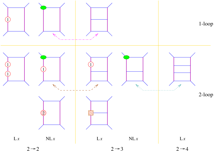
Figure 3.9: Cluster expansion. The various class of cut diagrams contributing to the 1-loop and 2-loops L$x$ + NL$x$ cross section are represented. Symmetric virtual correction diagrams are understood. The dashed/dotted lines joins classes of diagrams that are combined in order to form effective fragmentation vertices in the differential cross section.

The simplest process whose NL$x$ part of the kernel is identified is the elastic one (i). As Fig. 3.9 shows, there are three different 2-loops structures contributing at NL$x$ level: the leading gluon trajectory iteration, the product of gluon trajectory and PPR vertex correction and the pure NL$x$ gluon trajectory. The former, given in Eq. (2.32b), belongs to the iteration of the L$x$ kernel in Eq. (3.54). Also the PPR corrections, defined as the non logarithmic contribution to the 1-loop elastic amplitude has already been derived [29]. Therefore, the latter contribution, the NL$x$ gluon trajectory, can be unambiguously defined, by observing that in the elastic process the only physical scale is provided by the transferred momentum $-t\simeq{\boldsymbol{k}}^{2}$. In dimensional regularization $\Omega^{(1)}$ reads [38]

$$\Omega^{(1)}({\boldsymbol{k}}^{2}) =\frac{1}{8\varepsilon^{2}}\bigg{\{}-\left(\frac{{\boldsymbol{k}}^{2}}{\mu^{2}}\right)^{\varepsilon}\left({11N_{c}-2N_{\!f}\over 3N_{c}}-{11\pi^{2}\over 18}\varepsilon^{2}\right)+\left(\frac{{\boldsymbol{k}}^{2}}{\mu^{2}}\right)^{2\varepsilon}\left[\frac{11N_{c}-2N_{\!f}}{6N_{c}}\right.$$

$$\left.+\left(\frac{\pi^{2}}{6}-\frac{67}{18}+{5N_{\!f}\over 9N_{c}}\right)\varepsilon+\left(\frac{202}{27}-\frac{11\pi^{2}}{18}-\zeta(3)-{28N_{\!f}\over 27N_{c}}\right)\varepsilon^{2}\right]\bigg{\}}\;.$$ (3.55)

Three-particle final states

When considering one-particle production, the full amplitude with 1-loop corrections can be written [39]

$$M_{2\to 3}^{(1)}=M_{2\to 3}^{(0)}\bigg{\{}1+\bar{\alpha}_{\mathrm{s}}\bigg{[}\Pi_{\text{\sf a}\text{\sf a}}^{(+)}({\boldsymbol{k}}_{1}^{2})+\Pi_{\text{\sf b}\text{\sf b}}^{(+)}({\boldsymbol{k}}_{2}^{2})$$

$$+\frac{1}{2}\Omega^{(0)}({\boldsymbol{k}}_{1}^{2})\left(\ln\frac{s_{1}}{q^{2}}+\ln\frac{s_{1}}{k_{1}k_{2}}\right)+\frac{1}{2}\Omega^{(0)}({\boldsymbol{k}}_{2}^{2})\left(\ln\frac{s_{2}}{q^{2}}+\ln\frac{s_{2}}{k_{1}k_{2}}\right)\bigg{]}\bigg{\}}+\tilde{M}^{(1)}_{2\to 3}$$ (3.56)

where $M_{2\to 3}^{(0)}$ is given in Eq. (2.38), $s_{1}$ and $s_{2}$ are the sub-energies variables defined in Eq. (2.41), $\Pi$ is the vertex corrections of Eqs. (3.24,3.25,3.37) and $\tilde{M}^{(1)}_{2\to 3}$ is the reggeon-reggeon-gluon (RRG) vertex correction amplitude.

The RRG vertex corrections [40] didn’t take place in the 1-loop evaluation of the cross section and their interference with the Born amplitude $M_{2\to 3}^{(0)}$ give a pure NL$x$ contribution to 2-loops. On the contrary, the trajectory and PPR corrections are important in the 1-loop expansion (3.12) contributing to both the L$x$ and NL$x$ term, as explained in Sec. 3.4. Therefore, $\tilde{M}^{(1)}_{2\to 3}$ provides a so called “irreducible” contribution to the NL$x$ kernel, whereas the remaining terms of $M_{2\to 3}^{(1)}$ contribute to the NL$x$ kernel after the subtractions of the leading term, of the impact factor corrections and of the impact kernels.

The three ensuing structure contributing to the 2-loops cross section ($\Pi^{(+)},\Omega^{(0)}$ and $\tilde{M}$) are drawn in Fig. 3.9. The one-gluon irreducible contribution is given by [39]

$${{\rm d}\sigma^{(2,\text{irr})}_{2\to 3}\over{\rm d}{\boldsymbol{k}}_{1}\,{\rm d}{\boldsymbol{k}}_{2}} =\bar{\alpha}_{\mathrm{s}}^{2}h_{\text{\sf a}}^{(0)}\,K_{1\text{\sf g}}^{(\text{irr})}\ln{s\over k_{1}k_{2}}\,h_{\text{\sf b}}^{(0)}\;,$$ (3.57)

$$K_{1\text{\sf g}}^{(\text{irr})} =\frac{1}{4}\left[-{2\pi\over\varepsilon\pi_{\varepsilon}}\frac{({\boldsymbol{q}}^{2}/\mu^{2})^{\varepsilon}}{{\boldsymbol{q}}^{2}}\frac{\cos\pi\varepsilon}{\sin\pi\varepsilon}+\frac{11}{3}\left(\frac{1}{\varepsilon\pi_{\varepsilon}{\boldsymbol{q}}^{2}}+\frac{1}{{\boldsymbol{k}}_{1}^{2}-{\boldsymbol{k}}_{2}^{2}}\ln\frac{{\boldsymbol{k}}_{1}^{2}}{{\boldsymbol{k}}_{2}^{2}}\right)\right]\;,$$

where, for simplicity, an azimuthal average has been performed.

We now consider the one-particle emission with trajectory corrections diagrams together with the elastic ones carrying one PPR and one trajectory correction, as the dashed line in Fig. 3.9 indicates.

Let’s restrict to particle emission in the positive rapidity half space $y>0$ and let’s take the elastic diagrams with PPR correction only in the upper line, as in Fig. 3.10, the lower impact factor having been omitted. The first two diagrams are nothing but the components of the effective fragmentation vertex (cfr. Fig. 3.8) times the leading virtual term $\Omega^{(1)}\ln s$ in Eq. (3.5.1) and yield

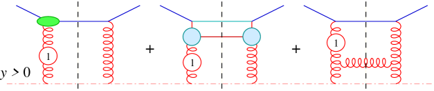
Figure 3.10: Reducible contribution to the NL$x$ kernel from three-particle final states: PPR corrections in the upper line (the symmetric virtual correction is understood) and real emission in the positive rapidity half space $y>0$ with 1-loop reggeon correction in the lower and upper propagator.

$${{\rm d}\sigma^{(2)}_{2\to 3}\over{\rm d}{\boldsymbol{k}}_{1}\,{\rm d}{\boldsymbol{k}}_{2}}\Big{|}_{\text{\sl a+b}}^{y>0} =h_{\text{\sf b}}^{(0)}({\boldsymbol{k}}_{2})\int_{q/\sqrt{s}}^{1}{\rm d}z_{1}\;F_{\text{\sf a}}(z_{1},{\boldsymbol{k}}_{1},{\boldsymbol{q}}){1\over 2}\Omega^{(0)}({\boldsymbol{k}}_{2}^{2})\left[\ln{s_{2}\over q^{2}}+\ln{s_{2}\over k_{1}k_{2}}\right]$$

$$=h_{\text{\sf b}}^{(0)}({\boldsymbol{k}}_{2})\Omega^{(0)}({\boldsymbol{k}}_{2}^{2})\int_{q/\sqrt{s}}^{1}{\rm d}z_{1}\;F_{\text{\sf a}}(z_{1},{\boldsymbol{k}}_{1},{\boldsymbol{q}})\ln{zs\over q\sqrt{k_{1}k_{2}}}\;,$$ (3.58)

since $s_{2}\simeq z_{1}s$. It is easy to realize that we get $\ln s$ terms from both the integration boundaries if you replace the NL$x$ fragmentation vertex with the leading one

$$F_{\text{\sf a}}(z,{\boldsymbol{k}},{\boldsymbol{q}})\raisebox{-5.69054pt}{\rule{0.2pt}{17.07164pt}}_{\,\text{L}x}={1\over z}\,{\bar{\alpha}_{\mathrm{s}}\over\pi_{\varepsilon}{\boldsymbol{q}}^{2}}$$ (3.59)

and perform the $z$-integration. Therefore, the effective vertex $F_{\text{\sf a}}$ provides an important NL$x$ correction with respect to its L$x$ analogue.

On the other hand, the third diagram in Fig. 3.10 yields

$${{\rm d}\sigma^{(2)}_{2\to 3}\over{\rm d}{\boldsymbol{k}}_{1}\,{\rm d}{\boldsymbol{k}}_{2}}\Big{|}_{\text{\sl c}}^{y>0} =h_{\text{\sf b}}^{(0)}({\boldsymbol{k}}_{2})\int_{q/\sqrt{s}}^{1}{\rm d}z_{1}\;\widetilde{F}_{\text{\sf a}}(z_{1},{\boldsymbol{k}}_{1},{\boldsymbol{q}}){1\over 2}\Omega^{(0)}({\boldsymbol{k}}_{1}^{2})\left[\ln{s_{1}\over q^{2}}+\ln{s_{1}\over k_{1}k_{2}}\right]$$

$$=h_{\text{\sf b}}^{(0)}({\boldsymbol{k}}_{2})\Omega^{(0)}({\boldsymbol{k}}_{1}^{2})\int_{q/\sqrt{s}}^{1}{\rm d}z_{1}\;\widetilde{F}_{\text{\sf a}}(z_{1},{\boldsymbol{k}}_{1},{\boldsymbol{q}})\ln{q\over z_{1}\sqrt{k_{1}k_{2}}}\;,$$ (3.60)

since $s_{1}\simeq q^{2}/z_{1}$. Here $\widetilde{F}_{\text{\sf a}}$ is another effective fragmentation vertex which, just like $F_{\text{\sf a}}$, reduces to the RHS of Eq. (3.59) in the small $z$-region and for all values of $z>q/\sqrt{s}$ in L$x$ approximation.

However, Eq. (3.60) provides a logarithmic contribution only in the vicinity of the lower integration boundary, and by making the substitution (3.59) for $\tilde{F}_{\text{\sf a}}$, the error is only NNL$x$.

In this way, by taking the derivative of Eqs. (3.58,3.60) with respect to $\ln s$ and by using Eq. (3.48), we can perform the $z_{1}$-integration exactly obtaining

$${\partial\over\partial\ln s}{{\rm d}\sigma^{(2)}_{2\to 3}\over{\rm d}{\boldsymbol{k}}_{1}\,{\rm d}{\boldsymbol{k}}_{2}} \Big{|}_{\text{\sl a+b+c}}^{y>0}$$ (3.61)

$$=\left\{\left[\left({\Omega_{1}\over 2}+{3\Omega_{2}\over 2}\right)\ln{s\over k_{1}k_{2}}+\Omega_{2}\ln{k_{2}\over k_{1}}+2\Omega_{2}\eta_{1}\right]{\bar{\alpha}_{\mathrm{s}}\over\pi_{\varepsilon}{\boldsymbol{q}}^{2}}+2\Omega_{2}H_{L}\right\}h_{\text{\sf b}}^{(0)}$$

where we have set $\Omega_{i}\,\raisebox{0.37pt}{:}=\Omega^{(0)}({\boldsymbol{k}}_{i}^{2})$ and $\eta_{i}\,\raisebox{0.37pt}{:}=\eta_{\text{\sf a}_{i}}({\boldsymbol{k}}_{i},{\boldsymbol{q}})$. Including the other half phase space $y<0$ ($\{1\leftrightarrow 2\},\{L\leftrightarrow R\}$), inverting the $\ln s$ derivative and carrying out the transverse integration of the $\eta$-terms in order to reproduce the impact factor corrections, we end up with the “reducible” part of the one-particle emission cross section [25]

$${{\rm d}\sigma^{(2,\text{red})}_{2\to 3}\over{\rm d}{\boldsymbol{k}}_{1}\,{\rm d}{\boldsymbol{k}}_{2}} =h_{\text{\sf a}}^{(0)}\left\{(\Omega_{1}+\Omega_{2}){\bar{\alpha}_{\mathrm{s}}\over\pi_{\varepsilon}{\boldsymbol{q}}^{2}}\ln^{2}{s\over k_{1}k_{2}}\right.$$ (3.62)

$$\quad+\left.\left[(\Omega_{1}-\Omega_{2}){\bar{\alpha}_{\mathrm{s}}\over\pi_{\varepsilon}{\boldsymbol{q}}^{2}}\ln{k_{1}\over k_{2}}+H_{L}2\Omega_{2}+2\Omega_{1}H_{R}\right]\ln{s\over k_{1}k_{2}}\right\}h_{\text{\sf b}}^{(0)}$$

$$\quad+\left[h_{\text{\sf a}}^{(0)}2\Omega_{1}{\bar{\alpha}_{\mathrm{s}}\over\pi_{\varepsilon}{\boldsymbol{q}}^{2}}h_{\text{\sf b}}^{(1)}+h_{\text{\sf a}}^{(1)}{\bar{\alpha}_{\mathrm{s}}\over\pi_{\varepsilon}{\boldsymbol{q}}^{2}}2\Omega_{2}h_{\text{\sf b}}^{(0)}\right]\ln{s\over k_{1}k_{2}}\;.$$

Four-particle final states

There remains to consider two-particle production at Born level (and the left over class of diagrams of the previous section). The contribution coming from a $\text{\sf q}\bar{\text{\sf q}}$ pair in the final state does not require any particular identification procedure, since it doesn’t appear at L$x$ level, giving therefore an irreducible contribution [41]:

$$\left.{{\rm d}\sigma^{(2)}_{2\to 4}\over{\rm d}{\boldsymbol{k}}_{1}\,{\rm d}{\boldsymbol{k}}_{2}}\right|_{\text{\sf q}\bar{\text{\sf q}}} =\bar{\alpha}_{\mathrm{s}}^{2}\,h_{\text{\sf a}}^{(0)}\,K^{(\text{irr})}_{\text{\sf q}\bar{\text{\sf q}}}\ln{s\over k_{1}k_{2}}\,h_{\text{\sf b}}^{(0)}$$ (3.63)

$$K^{(\text{irr})}_{\text{\sf q}\bar{\text{\sf q}}}({\boldsymbol{k}}_{1},{\boldsymbol{k}}_{2}) ={N_{\!f}\over 6N_{c}}\left[\left(\ln{{\boldsymbol{q}}^{2}\over\mu^{2}}-{5\over 3}\right){1\over{\boldsymbol{q}}^{2}}-{1\over{\boldsymbol{k}}_{1}^{2}-{\boldsymbol{k}}_{2}^{2}}\ln{{\boldsymbol{k}}_{1}^{2}\over{\boldsymbol{k}}_{2}^{2}}\right]\;.$$ (3.64)

The two-gluon production, on the contrary, gives L$x$ and NL$x$ contributions, and a treatment similar to that of Sec. 3.5.1 has to be done. First of all, we identify another irreducible contribution to the kernel, which consists in the production of a gluon pair in the central region with a small invariant mass.

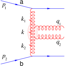
Figure 3.11: Two-gluon emission in the central region in QMRK.

To be explicit, according to Fig. 3.11, we parametrize the exchanged momenta by

$$k_{i}^{\mu} =z_{i}p_{1}^{\mu}+\bar{z}_{i}p_{2}^{\mu}+{\boldsymbol{k}}_{i}^{\mu}\qquad(i=1,2)\;,$$ (3.65a)

$$k^{\mu} =zp_{1}^{\mu}+\bar{z}p_{2}^{\mu}+{\boldsymbol{k}}^{\mu}$$ (3.65b)

so that the interesting kinematic region corresponds to the QMRK

$$1\gg z_{1}\sim z\gg z_{2}\simeq{{\boldsymbol{k}}_{2}^{2}\over s}\;.$$ (3.66)

The irreducible contribution to the $2\to 4$ cross section is then defined by subtracting, in the region (3.66), the leading term:

$${{\rm d}\sigma^{(2,\text{irr})}_{2\to 4}\over{\rm d}{\boldsymbol{k}}_{1}{\rm d}{\boldsymbol{k}}_{2}{\rm d}z_{1}{\rm d}z}={{\rm d}\sigma^{(2,\text{tot})}_{2\to 4}\over{\rm d}{\boldsymbol{k}}_{1}{\rm d}{\boldsymbol{k}}_{2}{\rm d}z_{1}{\rm d}z}-h_{\text{\sf a}}^{(0)}({\boldsymbol{k}}_{1})h_{\text{\sf b}}^{(0)}({\boldsymbol{k}}_{2}){1\over z_{1}}{1\over z}\int{\rm d}{\boldsymbol{k}}\;{\bar{\alpha}_{\mathrm{s}}\over\pi_{\varepsilon}{\boldsymbol{q}}_{1}^{2}}{\bar{\alpha}_{\mathrm{s}}\over\pi_{\varepsilon}{\boldsymbol{q}}_{2}^{2}}\;.$$ (3.67)

The irreducible contribution to the cross section is [42, 39]

$${{\rm d}\sigma^{(2,\text{irr})}_{2\to 4}\over{\rm d}{\boldsymbol{k}}_{1}\,{\rm d}{\boldsymbol{k}}_{2}}=\bar{\alpha}_{\mathrm{s}}^{2}h_{\text{\sf a}}^{(0)}\,K_{2\text{\sf g}}^{(\text{irr})}\ln{s\over k_{1}k_{2}}\,h_{\text{\sf b}}^{(0)}$$ (3.68)

in terms of the two-gluon irreducible kernel [42, 39]

$$K_{2\text{\sf g}}^{(\text{irr})} =\frac{1}{4}\bigg{\{}{2\Gamma^{2}(1+\varepsilon)\over\varepsilon\Gamma(1+2\varepsilon)\pi_{\varepsilon}}\frac{({\boldsymbol{q}}^{2}/\mu^{2})^{\varepsilon}}{{\boldsymbol{q}}^{2}}\left[\frac{1}{\varepsilon}-\frac{11}{6}+\left(\frac{67}{18}-\frac{\pi^{2}}{2}\right)\varepsilon-\left(\frac{202}{27}-7\zeta(3)\right)\varepsilon^{2}\right]$$

$$-H_{\text{coll}}({\boldsymbol{k}}_{1},{\boldsymbol{k}}_{2})+\tilde{H}({\boldsymbol{k}}_{1},{\boldsymbol{k}}_{2})\bigg{\}}\;,$$ (3.69)

where we have introduced the “collinear” kernel

$$H_{\text{coll}}({\boldsymbol{k}}_{1},{\boldsymbol{k}}_{2})=\frac{1}{32\pi}\left[2\left(\frac{1}{{\boldsymbol{k}}_{1}^{2}}+\frac{1}{{\boldsymbol{k}}_{2}^{2}}\right)+\left(\frac{1}{{\boldsymbol{k}}_{2}^{2}}-\frac{1}{{\boldsymbol{k}}_{1}^{2}}\right)\ln\frac{{\boldsymbol{k}}_{1}^{2}}{{\boldsymbol{k}}_{2}^{2}}+\left(118-\frac{{\boldsymbol{k}}_{1}^{2}}{{\boldsymbol{k}}_{2}^{2}}-\frac{{\boldsymbol{k}}_{2}^{2}}{{\boldsymbol{k}}_{1}^{2}}\right)\times\right.$$

$$\left.\times\frac{1}{\sqrt{{\boldsymbol{k}}_{1}^{2}{\boldsymbol{k}}_{2}^{2}}}\left(\ln\frac{{\boldsymbol{k}}_{1}^{2}}{{\boldsymbol{k}}_{2}^{2}}\tan^{-1}\frac{|{\boldsymbol{k}}_{2}|}{|{\boldsymbol{k}}_{1}|}+\operatorname{\Im\text{m}}\text{Li}_{2}\left({\rm i}\frac{|{\boldsymbol{k}}_{2}|}{|{\boldsymbol{k}}_{1}|}\right)\right)\right]-\frac{\pi^{2}}{3k^{2}_{>}},$$ (3.70)

in which an azimuthal average has been performed, and the dilogarithmic one

$$\tilde{H}({\boldsymbol{k}}_{1},{\boldsymbol{k}}_{2})=-\frac{\pi}{3k_{>}^{2}}+\frac{2{\boldsymbol{q}}\cdot({\boldsymbol{k}}_{1}+{\boldsymbol{k}}_{2})}{\pi{\boldsymbol{q}}^{2}({\boldsymbol{k}}_{1}+{\boldsymbol{k}}_{2})^{2}}\left[\ln\frac{{\boldsymbol{k}}_{1}^{2}}{{\boldsymbol{k}}_{2}^{2}}\ln\frac{{\boldsymbol{k}}_{1}^{2}{\boldsymbol{k}}_{2}^{2}}{({\boldsymbol{k}}_{1}^{2}+{\boldsymbol{k}}_{2}^{2})^{2}}+\right.$$

$$\left.+\text{Li}_{2}\left(1-\frac{{\boldsymbol{q}}^{2}}{{\boldsymbol{k}}_{1}^{2}}\right)-\text{Li}_{2}\left(1-\frac{{\boldsymbol{q}}^{2}}{{\boldsymbol{k}}_{2}^{2}}\right)+\text{Li}_{2}\left(-\frac{{\boldsymbol{k}}_{2}^{2}}{{\boldsymbol{k}}_{1}^{2}}\right)-\text{Li}_{2}\left(-\frac{{\boldsymbol{k}}_{1}^{2}}{{\boldsymbol{k}}_{2}^{2}}\right)\right]+$$

$$+{2\over\pi}\left[\int_{0}^{1}\frac{dt}{({\boldsymbol{k}}_{1}-t{\boldsymbol{k}}_{2})^{2}}\left(\frac{{\boldsymbol{k}}_{2}\cdot{\boldsymbol{q}}}{{\boldsymbol{q}}^{2}}-\frac{{\boldsymbol{k}}_{2}^{2}{\boldsymbol{q}}\cdot({\boldsymbol{k}}_{1}+{\boldsymbol{k}}_{2})}{{\boldsymbol{q}}^{2}({\boldsymbol{k}}_{1}+{\boldsymbol{k}}_{2})^{2}}(1+t)\right)\ln\frac{t(1-t){\boldsymbol{k}}_{2}^{2}}{{\boldsymbol{k}}_{1}^{2}(1-t)+{\boldsymbol{q}}^{2}t}+\right.$$

$$+({\boldsymbol{k}}_{1}\longleftrightarrow-{\boldsymbol{k}}_{2})\bigg{]}.$$ (3.71)

where $k_{>}^{2}\,\raisebox{0.37pt}{:}=\operatorname{{\rm Max}}({\boldsymbol{k}}_{1}^{2},{\boldsymbol{k}}_{2}^{2})$.

At this point, to complete the calculation, it remains to evaluate the subtracted term in the RHS of Eq. (3.67) to NL$x$ accuracy. To do this, we add to it the one-particle emission diagrams with PPR corrections (see the dotted line in Fig. 3.9) and perform the following analysis: let $q_{1}$ be the gluon with the largest rapidity and define

$$y_{i}\,\raisebox{0.37pt}{:}=\ln z_{i}{\sqrt{s}\over q_{i}}\quad,\quad y_{i}\in[-Y_{i},Y_{i}]\quad,\quad Y_{i}\,\raisebox{0.37pt}{:}=\ln{\sqrt{s}\over q_{i}}\;.$$ (3.72)

Working at fixed transverse momenta, we split the phase space into three regions:

$$A: 0 <y_{2}<y_{1}<Y_{1}\;,$$

$$B: -Y_{2} <y_{2}<0<y_{1}<Y_{1}\;,$$

$$C: -Y_{2} <y_{2}<y_{1}<0\;.$$

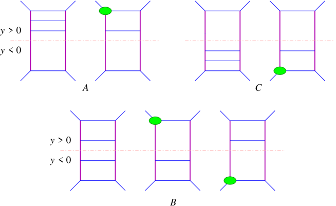
Figure 3.12: How $2\to 3$ and $2\to 4$ diagrams are combined in order to reconstruct the effective fragmentation vertices. Symmetric virtual corrections diagrams are understood.

Then we add the one-particle emission diagrams with PPR corrections that we distinguish into four types — according to the sign of the rapidity of the emitted particle and to the (upper or lower) leg which the PPR correction is attached to — and we associate them to the three regions $A,B$ and $C$ as in Fig. 3.12. Repeating the analysis of Sec. 3.5.1 we reproduce the effective fragmentation vertex in the relevant phase space regions, and remembering that, when $y_{1}\simeq y_{2}$ the subtracted term is exactly given by the last one in Eq. (3.67), we are allowed to write, at NL$x$ accuracy,

$${{\rm d}\sigma^{(2,\text{red})}_{2\to 4}\over{\rm d}{\boldsymbol{k}}_{1}\,{\rm d}{\boldsymbol{k}}_{2}} =h_{\text{\sf a}}^{(0)}({\boldsymbol{k}}_{1})h_{\text{\sf b}}^{(0)}({\boldsymbol{k}}_{2})\int{\rm d}{\boldsymbol{k}}\;{\bar{\alpha}_{\mathrm{s}}\over\pi_{\varepsilon}{\boldsymbol{q}}_{1}^{2}}{\bar{\alpha}_{\mathrm{s}}\over\pi_{\varepsilon}{\boldsymbol{q}}_{2}^{2}}\big{(}\rho_{A}+\rho_{B}+\rho_{C})\;,$$ (3.73)

where

$$\rho_{A} =\int_{q_{1}/\sqrt{s}}^{1}{{\rm d}z_{1}\over z_{1}}\;{\mathcal{F}}_{\text{\sf a}}(z_{1},{\boldsymbol{k}}_{1},{\boldsymbol{q}}_{1})\int_{q_{2}/\sqrt{s}}^{\operatorname{{\rm Min}}\big{(}1,{q_{2}\over q_{1}}z_{1}\big{)}}{{\rm d}z\over z}\;,$$

$$\rho_{B} =\int_{q_{1}/\sqrt{s}}^{1}{{\rm d}z_{1}\over z_{1}}\;{\mathcal{F}}_{\text{\sf a}}(z_{1},{\boldsymbol{k}}_{1},{\boldsymbol{q}}_{1})\int_{q_{2}/\sqrt{s}}^{1}{{\rm d}\bar{z}_{2}\over\bar{z}_{2}}\;{\mathcal{F}}_{\text{\sf b}}(\bar{z}_{2},{\boldsymbol{k}}_{2},{\boldsymbol{q}}_{2})\;,$$

$$\rho_{C} =\int_{q_{2}/\sqrt{s}}^{1}{{\rm d}\bar{z}_{2}\over\bar{z}_{2}}\;{\mathcal{F}}_{\text{\sf b}}(\bar{z}_{2},{\boldsymbol{k}}_{2},{\boldsymbol{q}}_{2})\int_{q_{1}/\sqrt{s}}^{\operatorname{{\rm Min}}\big{(}1,{q_{1}\over q_{2}}\bar{z}_{2}\big{)}}{{\rm d}\bar{z}\over\bar{z}}=\rho_{A}|_{1\leftrightarrow 2}^{\text{\sf a}\leftrightarrow\text{\sf b}}$$

and the “reduced” fragmentation vertex ${\mathcal{F}}_{\text{\sf a}}$ is

$$F_{\text{\sf a}}(z,{\boldsymbol{k}},{\boldsymbol{q}})=\raisebox{0.37pt}{:}\hskip 3.0pth_{\text{\sf a}}^{(0)}({\boldsymbol{k}}){\bar{\alpha}_{\mathrm{s}}\over\pi_{\varepsilon}{\boldsymbol{q}}^{2}}{\mathcal{F}}_{\text{\sf a}}(z,{\boldsymbol{k}},{\boldsymbol{q}})\;.$$ (3.74)

By deriving with respect to $\ln s$, performing the integrals and inserting the results in Eq. (3.73), we obtain [25]

$${{\rm d}\sigma^{(2,\text{red})}_{2\to 4}\over{\rm d}{\boldsymbol{k}}_{1}\,{\rm d}{\boldsymbol{k}}_{2}} =h_{\text{\sf a}}^{(0)}h_{\text{\sf b}}^{(0)}\left\{{1\over 2}\ln^{2}{s\over k_{1}k_{2}}\;{\bar{\alpha}_{\mathrm{s}}\over\pi_{\varepsilon}{\boldsymbol{q}}_{1}^{2}}\circ{\bar{\alpha}_{\mathrm{s}}\over\pi_{\varepsilon}{\boldsymbol{q}}_{2}^{2}}\ln{s\over k_{1}k_{2}}\left[H_{L}\circ{\bar{\alpha}_{\mathrm{s}}\over\pi_{\varepsilon}{\boldsymbol{q}}_{2}^{2}}+{\bar{\alpha}_{\mathrm{s}}\over\pi_{\varepsilon}{\boldsymbol{q}}_{1}^{2}}\circ H_{R}\right]\right\}$$

$$\quad+\ln{s\over k_{1}k_{2}}\left[h_{\text{\sf a}}^{(0)}{\bar{\alpha}_{\mathrm{s}}\over\pi_{\varepsilon}{\boldsymbol{q}}_{1}^{2}}h_{\text{\sf b}}^{(1)}+h_{\text{\sf a}}^{(1)}{\bar{\alpha}_{\mathrm{s}}\over\pi_{\varepsilon}{\boldsymbol{q}}_{2}^{2}}h_{\text{\sf b}}^{(0)}\right]\;,$$ (3.75)

the small circle $\circ$ denoting composition of operators, i.e., a ${\boldsymbol{k}}$-integration.

3.5.2 Next-to-leading BFKL kernel

The left over elastic contributions (the first and the third diagram in the $2\to 2$, 2-loops group of Fig. 3.9) contribute to the cross section with

$${{\rm d}\sigma^{(2)}_{2\to 2}\over{\rm d}{\boldsymbol{k}}_{1}\,{\rm d}{\boldsymbol{k}}_{2}}=h_{\text{\sf a}}^{(0)}h_{\text{\sf b}}^{(0)}\delta({\boldsymbol{k}}_{1}-{\boldsymbol{k}}_{2})\left\{{1\over 2}\big{(}2\Omega_{1}2\Omega_{2}\big{)}\ln^{2}{s\over k_{1}k_{2}}+2\Omega^{(1)}({\boldsymbol{k}}_{1}^{2})\ln{s\over k_{1}k_{2}}\right\}\;.$$ (3.76)

At least we are at the final step: by adding Eqs. (3.57,3.62,3.63,3.68,3.75,3.76) and identifying the corresponding terms in the expansion (3.54), we are able to single out the NL$x$ BFKL kernel at energy-scale $s_{0}=k_{1}k_{2}$ [24, 25]:

$$K^{(1)} =2\Omega^{(1)}({\boldsymbol{k}}_{1}^{2})\delta({\boldsymbol{k}}_{1}-{\boldsymbol{k}}_{2})+K_{1\text{\sf g}}^{(\text{irr})}+K_{\text{\sf q}\bar{\text{\sf q}}}^{(\text{irr})}+K_{2\text{\sf g}}^{(\text{irr})}+{\Omega_{1}-\Omega_{2}\over({\boldsymbol{k}}_{1}-{\boldsymbol{k}}_{2})^{2}}\ln{k_{1}\over k_{2}}$$

$$=-b_{0}\ln{{\boldsymbol{k}}_{1}^{2}\over\mu^{2}}\,K^{(0)}+K^{(1)}_{\text{s.i.}}$$ (3.77)

where in the second line we have explicitly shown the scale-invariance violating term and $K^{(1)}_{\text{s.i.}}$ defines the scale-invariant part of the NL$x$ kernel. Note that the coefficient of the $\ln\mu^{2}$ term is precisely the leading kernel with the $\beta$-function coefficient $b_{0}$ given in Eq. (1.2). Therefore it can be interpreted as a running factor and we can express the total L$x$ + NL$x$ kernel in the form

$${\mathcal{K}} =\bar{\alpha}_{\mathrm{s}}(\mu^{2})\left[\big{(}1-b_{0}\alpha_{\mathrm{s}}(\mu^{2})\ln{{\boldsymbol{k}}_{1}^{2}\over\mu^{2}}\big{)}\right]K^{(0)}+\bar{\alpha}_{\mathrm{s}}(\mu^{2})K^{(1)}_{\text{s.i.}}$$ (3.78a)

$$=\bar{\alpha}_{\mathrm{s}}({\boldsymbol{k}}_{1}^{2})\big{[}K^{(0)}+\bar{\alpha}_{\mathrm{s}}(\mu^{2})K^{(1)}_{\text{s.i.}}\big{]}+{\mathcal{O}}(\alpha_{\mathrm{s}}^{3})$$ (3.78b)

Factorizing the running coupling at the scale ${\boldsymbol{k}}_{1}^{2}$ is an asymmetric procedure, but is convenient for the discussion of the non-scale-invariant BFKL equation. Using a different scale (e.g., $\alpha_{\mathrm{s}}(k_{>}^{2})$) implies changing $K^{(1)}_{\text{s.i.}}$ so as to leave the total NL kernel invariant (see below).

3.5.3 Eigenvalues of the NL$x$ kernel

In order to investigate the physical features emerging from the NL$x$ kernel, we determine the eigenvalues of the scale-invariant part by applying ${\mathcal{K}}$ to the (spherically symmetric) eigenfunctions of the leading kernel:

$$\bar{\alpha}_{\mathrm{s}}({\boldsymbol{k}}^{2})\!\int\!{\rm d}{\boldsymbol{k}}^{\prime}\big{(}K^{(0)}({\boldsymbol{k}},{\boldsymbol{k}}^{\prime})+\bar{\alpha}_{\mathrm{s}}K^{(1)}_{\text{s.i.}}({\boldsymbol{k}},{\boldsymbol{k}}^{\prime})\big{)}({\boldsymbol{k}}^{\prime}{}^{2})^{\gamma-1}=\bar{\alpha}_{\mathrm{s}}({\boldsymbol{k}}^{2})\left[\chi^{(0)}(\gamma)+\bar{\alpha}_{\mathrm{s}}\chi^{(1)}(\gamma)\right]({\boldsymbol{k}}^{\prime}{}^{2})^{\gamma-1}\,.$$ (3.79)

The leading eigenvalue $\chi^{(0)}$ is the same of Eq. (2.60) with $m=0$:

$$\chi^{(0)}(\gamma)=2\psi(1)-\psi(\gamma)-\psi(1-\gamma)\;,$$ (3.80)

while the eigenvalue function $\chi^{(1)}$ of the next-to-leading kernel $K^{(1)}_{\text{s.i.}}$ ($\equiv K^{(1)}$ from now on) is the sum of a gluonic part

$$\chi^{(1,\text{\sf g})}(\gamma)= -{1\over 2}\bigg{[}{11\over 12}\big{(}\chi^{(0)\,2}(\gamma)+\chi^{(0)}{}^{\prime}(\gamma)\big{)}\bigg{]}-{1\over 4}\chi^{(0)}{}^{\prime\prime}(\gamma)$$ (3.81)

$$-\left({\pi\over\sin\pi\gamma}\right)^{2}{\cos\pi\gamma\over(1-2\gamma)}\left({11\over 12}+{\gamma(1-\gamma)\over 36(1+2\gamma)(1-{2\over 3}\gamma)}\right)$$

$$+\left({67\over 36}-{\pi^{2}\over 12}\right)\chi^{(0)}(\gamma)+{3\over 2}\,\zeta(3)+{\pi^{3}\over 4\sin\pi\gamma}-\Phi(\gamma)\;,$$

$$\Phi(\gamma)\,\raisebox{0.37pt}{:}=\sum_{n=0}^{\infty} (-)^{n}\left[{\psi(n+1+\gamma)-\psi(1)\over(n+\gamma)^{2}}+{\psi(n+2-\gamma)-\psi(1)\over(n+1-\gamma)^{2}}\right]\;,$$ (3.82)

and a quark — $N_{\!f}$-dependent — one

$$\chi^{(1,\text{\sf q})}(\gamma)={N_{\!f}\over 6N_{c}}\bigg{[} {1\over 2}\big{(}\chi^{(0)\,2}(\gamma)+\chi^{(0)}{}^{\prime}(\gamma)\big{)}-{5\over 3}\chi^{(0)}(\gamma)$$ (3.83)

$$-{1\over N_{c}^{2}}\left({\pi\over\sin\pi\gamma}\right)^{2}{\cos\pi\gamma\over 1-2\gamma}\,{1+{3\over 2}\gamma(1-\gamma)\over(1+2\gamma)(1-{2\over 3}\gamma)}\bigg{]}\;.$$

We want to stress that the particular form of the NL$x$ kernel, and hence the NL$x$ eigenvalue, depends on the choice of both the scale of $\bar{\alpha}_{\mathrm{s}}$ and the scale of the energy $s_{0}$. For instance, if we adopt $k_{>}^{2}$ as the argument of $\bar{\alpha}_{\mathrm{s}}$, in Eq. (3.77) we should replace

$$b\ln{k_{1}^{2}\over\mu^{2}}K^{(0)}=-b\ln{k_{>}^{2}\over\mu^{2}}K^{(0)}-b\Theta_{k_{2}\,k_{1}}\ln{k_{2}^{2}\over k_{1}^{2}}K^{(0)}\;,$$ (3.84)

so that the NL$x$ kernel undergoes a shift

$$\Delta K^{(1)}=-b\Theta_{k_{2}\,k_{1}}\ln{k_{2}^{2}\over k_{1}^{2}}K^{(0)}=-b{\Theta_{k_{2}\,k_{1}}\over|{\boldsymbol{k}}_{1}-{\boldsymbol{k}}_{2}|^{2}}\ln{k_{2}^{2}\over k_{1}^{2}}$$ (3.85)

and, correspondingly, the NL$x$ eigenvalue function acquires the additional term

$$\Delta\chi^{(1)}(\gamma)=-b\psi^{\prime}(1-\gamma)$$ (3.86)

which symmetrizes completely itself.

In DIS the energy dependence of the SF is commonly expressed by means of the Bjorken variable $x\simeq Q^{2}/s$, $s$ being the photon-proton CM energy squared. In the limit of $Q^{2}\gg{\boldsymbol{k}}_{0}^{2}$, where ${\boldsymbol{k}}_{0}^{2}$ is the typical transverse momentum scale of the proton’s constituents, the correct energy-scale is $s_{0}=k^{2}\sim Q^{2}$. The shift in the NL$x$ kernel corresponding to the change $s_{0}=kk_{0}\to k^{2}$ can be accomplished by a simple trick. If we denote with $H(\gamma)$ the eigenvalue function of the impact kernel $H$ of Eq. (3.51)

$$H(\gamma)=-{1\over 2}\sum_{n=0}^{\infty}\left({\Gamma(\gamma+n)\over\Gamma(\gamma)n!}\right)^{2}{1\over(\gamma+n)^{2}}\stackrel{{\scriptstyle\gamma\to 0}}{{=}}-{1\over 2\gamma^{2}}+{\mathcal{O}}(\gamma^{2})\;,$$ (3.87)

the GGF (actually, its scale-invariant part) has the representation (cfr. Eq. (2.61) with $m=0$)

$${\mathcal{G}}(s,k,k_{0}) =\int{{\rm d}\omega\over 2\pi{\rm i}}{{\rm d}\gamma\over 2\pi{\rm i}}\;\left({s\over kk_{0}}\right)^{\omega}g_{\omega}(\gamma)\left({k^{2}\over k_{0}^{2}}\right)^{\gamma}{1\over\pi k^{2}}$$ (3.88a)

$$=\int{{\rm d}\omega\over 2\pi{\rm i}}{{\rm d}\gamma\over 2\pi{\rm i}}\;\left({s\over k^{2}}\right)^{\omega}g_{\omega}(\gamma)\left({k^{2}\over k_{0}^{2}}\right)^{\gamma+\mbox{\small$\frac{1}{2}$}\omega}{1\over\pi k^{2}}$$ (3.88b)

where

$$g_{\omega}(\gamma) ={1+\bar{\alpha}_{\mathrm{s}}[H(\gamma)+H(1-\gamma)]\over\omega-\bar{\alpha}_{\mathrm{s}}\left[\chi^{(0)}(\gamma)+\bar{\alpha}_{\mathrm{s}}\chi^{(1)}(\gamma)\right]}\qquad(s_{0}=kk_{0})\;.$$ (3.88c)

Therefore the energy-scale change $kk_{0}\to k^{2}$ is equivalent to replacing $\gamma$ with $\gamma+\mbox{\small$\frac{1}{2}$}\omega$. By shifting $\gamma$ in $g_{\omega}$ and then expanding in $\omega$ up to NL$x$ level, the GGF Mellin transform at the “upper” energy-scale $s_{0}=k^{2}$ reads

$$g^{[u]}_{\omega}(\gamma)={1+\bar{\alpha}_{\mathrm{s}}[H(\gamma)-\mbox{\small$\frac{1}{2}$}\chi^{(0)}{}^{\prime}(\gamma)+H(1-\gamma)]\over\omega-\bar{\alpha}_{\mathrm{s}}\left[\chi^{(0)}(\gamma)+\bar{\alpha}_{\mathrm{s}}\chi^{(1)}(\gamma)-\mbox{\small$\frac{1}{2}$}\bar{\alpha}_{\mathrm{s}}\chi^{(0)}\chi^{(0)}{}^{\prime}\right]}\qquad(s_{0}=k^{2})\;.$$ (3.89)

This means that the shift in the kernel’s eigenvalue function is

$$\Delta\chi^{(1)}=-{1\over 2}\chi^{(0)}\chi^{(0)}{}^{\prime}\stackrel{{\scriptstyle\gamma\to 0}}{{=}}{1\over 2\gamma^{3}}-\zeta(3)+{\mathcal{O}}(\gamma^{2})\;.$$ (3.90)

The shift (3.90) cancels the cubic singularity (and the $\zeta(3)$ term) of

$$\chi^{(1)}(\gamma)\stackrel{{\scriptstyle\gamma\to 0}}{{=}} -{1\over 2\gamma^{3}}+{A_{1}\over\gamma^{2}}+{A_{2}\over\gamma}+A_{3}+\zeta(3)+{\mathcal{O}}(\gamma)\;,$$ (3.91)

$$A_{1} =-\left({11\over 12}+{N_{\!f}\over 6N_{c}^{3}}\right)\;,$$

$$A_{2} =-{N_{\!f}\over 6N_{c}}\left({5\over 3}+{13\over 6N_{c}^{2}}\right)\;,$$

$$A_{3} =-{1\over 4}\left[{395\over 27}-2\zeta(3)-{11\pi^{2}\over 18}+{N_{\!f}\over N_{c}^{3}}\left({71\over 27}-{\pi^{2}\over 9}\right)\right]\;,$$

providing the right collinear behaviour for $k^{2}\gg k_{0}^{2}$, as explained in the next section. Furthermore, by Eq. (3.87), the numerator in Eq. (3.89) becomes regular for $\gamma=0$ too, where it takes the value $1+\bar{\alpha}_{\mathrm{s}}H(1)=1-\bar{\alpha}_{\mathrm{s}}\psi^{\prime}(1)$, which renormalizes the impact factors. This confirms the importance of factorizing $H$ in the GGF in Eq. (3.53).

3.6 NL$x$ resummed anomalous dimension

In order to determine the resummed anomalous dimension in NL$x$ approximation, we have to check whether the NL$x$ BFKL equation is consistent with the RG equation. The running of the coupling spoils the arguments of Sec. 2.3.2 and a new analysis is needed.

The choice of $k^{2}$ as the scale of $\alpha_{\mathrm{s}}$ is suitable for that analysis. In fact, the inhomogeneous BFKL equation for the unintegrated gluon density (2.62) reads

$$\omega\left[{\mathcal{F}}_{\omega}({\boldsymbol{k}})-{\mathcal{F}}_{\omega}^{(0)}({\boldsymbol{k}})\right]={1\over b\ln{k^{2}\over\Lambda^{2}}}\int{\rm d}{\boldsymbol{k}}^{\prime}\;K({\boldsymbol{k}},{\boldsymbol{k}}^{\prime})\,{\mathcal{F}}_{\omega}({\boldsymbol{k}}^{\prime})\quad,\quad b\,\raisebox{0.37pt}{:}={\pi\over N_{c}}b\;,$$ (3.92)

where we have explicitly written the perturbative expression of the running coupling $\bar{\alpha}_{\mathrm{s}}(k^{2})$ and the scale-invariant L$x$ + NL$x$ kernel $K=K^{(0)}+\bar{\alpha}_{\mathrm{s}}K^{(1)}$. In $\gamma$-space, Eq. (3.92) assumes a simpler form: with the definition (C.19c) and by observing that $b\ln k^{2}/\Lambda^{2}\to-b\partial_{\gamma}$ and $K\to\chi=\chi^{(0)}+\bar{\alpha}_{\mathrm{s}}\chi^{(1)}$, we obtain

$$-b\omega[{\mathcal{F}}_{\omega}(\gamma)-{\mathcal{F}}_{\omega}^{(0)}(\gamma)]^{\prime}=\chi(\gamma){\mathcal{F}}_{\omega}(\gamma)\quad,\quad{\mathcal{F}}^{\prime}\equiv\partial_{\gamma}{\mathcal{F}}\;,$$ (3.93)

which is a first order linear differential equation for ${\mathcal{F}}_{\omega}$ admitting the formal solution [4]

$${\mathcal{F}}_{\omega}(\gamma) ={\rm e}^{-{X(\gamma)\over b\omega}}\int_{\infty}^{\gamma}{\rm d}\gamma^{\prime}\;{\rm e}^{X(\gamma^{\prime})\over b\omega}{\mathcal{F}}_{\omega}^{(0)}{}^{\prime}(\gamma^{\prime})\;,$$ (3.94a)

$${\mathcal{F}}_{\omega}({\boldsymbol{k}}) ={1\over\pi k^{2}}\int{{\rm d}\gamma\over 2\pi{\rm i}}\;\left({k^{2}\over\Lambda^{2}}\right)^{\gamma}{\mathcal{F}}_{\omega}(\gamma)\;,$$ (3.94b)

where $X$ is any primitive of $\chi$.

It has been argued [45, 43] that, in the limit $k^{2}\gg k_{0}^{2}$, the GGF assume the factorized form

$${\mathcal{G}}_{\omega}({\boldsymbol{k}},{\boldsymbol{k}}_{0})=F_{\omega}({\boldsymbol{k}})\widetilde{F}_{\omega}({\boldsymbol{k}}_{0})\times\left[1+{\mathcal{O}}\big{(}{k_{0}^{2}\over k^{2}}\big{)}\right]$$ (3.95)

where $F$ is purely perturbative while $\widetilde{F}$ is determined by the properties of non perturbative physics. After integration with the bare ${\boldsymbol{k}}_{0}$-dependent gluon distribution (Eq. (2.28)), the unintegrated gluon density ${\mathcal{F}}_{\omega}({\boldsymbol{k}})$ inherits the factorized form

$${\mathcal{F}}_{\omega}({\boldsymbol{k}})=F_{\omega}({\boldsymbol{k}})\widetilde{f}_{\omega}+\text{higher twist}\;.$$ (3.96)

A comparison with Eqs. (3.94) led us to identify the non perturbative factor

$$\widetilde{f}_{\omega}\simeq{1\over 2}\left(\int_{\infty-{\rm i}\varepsilon}^{0}+\int_{\infty+{\rm i}\varepsilon}^{0}\right){\rm d}\gamma^{\prime}\;{\rm e}^{X(\gamma^{\prime})\over b\omega}{\mathcal{F}}_{\omega}^{(0)}{}^{\prime}(\gamma^{\prime})\;,$$ (3.97)

where we have set the upper integration limit $\gamma\simeq 0$ (see below). The perturbative factor, on the other hand, carries the whole ${\boldsymbol{k}}$-dependence of ${\mathcal{F}}_{\omega}$ and is given by

$$F_{\omega}({\boldsymbol{k}})={1\over\pi k^{2}}\int{{\rm d}\gamma\over 2\pi{\rm i}}\;\left({k^{2}\over\Lambda^{2}}\right)^{\gamma}{\rm e}^{-{X(\gamma)\over b\omega}}\;.$$ (3.98)

In the anomalous dimension limit $k^{2}\gg\Lambda^{2}$, Eq. (3.98) can be evaluated by the saddle point method, which yields [44]

$$F_{\omega}({\boldsymbol{k}})\simeq{1\over k^{2}}\sqrt{b\omega\over 2\pi|\chi^{\prime}(\bar{\gamma})|}\exp\int^{t}\bar{\gamma}_{\omega}(\tau)\,{\rm d}\tau\qquad\big{(}t\,\raisebox{0.37pt}{:}=\ln{k^{2}\over\Lambda^{2}}\big{)}\;,$$ (3.99)

where $\bar{\gamma}=\bar{\gamma}_{\omega}(t)=\partial_{t}[\bar{\gamma}t-X(\bar{\gamma})/b\omega]$ is the position of the saddle point determined by the condition

$${\omega\over\bar{\alpha}_{\mathrm{s}}(t)}=b\omega t=\chi^{(0)}(\bar{\gamma})+\bar{\alpha}_{\mathrm{s}}\chi^{(1)}(\bar{\gamma})\;.$$ (3.100)

The representation (3.99) is valid only in the anomalous dimension regime

$$b\omega t\gg\chi_{m}\,\raisebox{0.37pt}{:}=\underset{\gamma\in]0,1[}{\operatorname{{\rm Min}}}\chi(\gamma)\;.$$ (3.101)

If the above limitation were not satisfied, the representation (3.99) would breaks down, due to large $\gamma$-fluctuations.

Finally, we consider the singlet density (2.27)

$$f_{\omega}^{(+)}(Q^{2}) =\int{{\rm d}\gamma\over 2\pi{\rm i}}\left({Q^{2}\over\Lambda^{2}}\right)^{\gamma}{{\mathcal{F}}_{\omega}(\gamma)\over\gamma}$$

$$={1\over\bar{\gamma}}\sqrt{b\omega\over 2\pi|\chi^{\prime}(\bar{\gamma})|}\exp\int^{t_{Q}}\bar{\gamma}_{\omega}(\tau)\,{\rm d}\tau\qquad\big{(}t_{Q}\,\raisebox{0.37pt}{:}=\ln{Q^{2}\over\Lambda^{2}}\big{)}\;.$$ (3.102)

The coefficient function in front of the exponential term is simply a constant in the $Q^{2}\to 0$ ($\bar{\gamma}\to 0$) limit and the singlet density satisfies

$${{\rm d}\over{\rm d}\ln Q^{2}}f_{\omega}^{(+)}(Q^{2})=\bar{\gamma}_{\omega}(Q^{2})f_{\omega}^{(+)}(Q^{2})\;,$$ (3.103)

consistently with the RG equation (1.36). Therefore, we interpret the function $\bar{\gamma}_{\omega}$ implicitly defined by (3.100) as the (highest eigenvalue of the) resummed anomalous dimension in the singlet sector.

The structure of the NL$x$ eigenvalue function at coupling-scale and energy-scale $k^{2}$ is (cfr. Eqs. (3.91,3.90))

$$\chi^{(1)}(\gamma) ={A_{1}\over\gamma^{2}}+{A_{2}\over\gamma}+A_{3}+{\mathcal{O}}(\gamma)$$ (3.104)

This imply that, up to 3-loops, the NL$x$ anomalous dimension has the expansion

$$\bar{\gamma}_{\omega}(\bar{\alpha}_{\mathrm{s}}) =\gamma_{\textsc{l}}\big{(}{\bar{\alpha}_{\mathrm{s}}\over\omega}\big{)}+\bar{\alpha}_{\mathrm{s}}\gamma_{\textsc{nl}}\big{(}{\bar{\alpha}_{\mathrm{s}}\over\omega}\big{)}\qquad\qquad\left(\gamma_{\textsc{nl}}={\chi^{(1)}(\gamma_{\textsc{l}})\over-\chi^{(0)}{}^{\prime}(\gamma_{\textsc{l}})}\right)$$ (3.105)

$$={\bar{\alpha}_{\mathrm{s}}\over\omega}+\bar{\alpha}_{\mathrm{s}}\left(A_{1}+A_{2}{\bar{\alpha}_{\mathrm{s}}\over\omega}+A_{3}{\bar{\alpha}_{\mathrm{s}}^{2}\over\omega^{2}}\right)+{\mathcal{O}}(\bar{\alpha}_{\mathrm{s}}^{4})$$ (3.106)

which can be checked to be consistent with the known expression up to ${\mathcal{O}}(\alpha_{\mathrm{s}}^{2})$. It is apparent that, in order to recover the expansion (3.106), the double pole of $\chi^{(1)}$, and hence the shift to scale $s_{0}=k^{2}$, plays a crucial role: if a cubic singularity were been present, the anomalous dimension would assume the non realistic form $\bar{\gamma}\simeq\bar{\alpha}_{\mathrm{s}}^{2/3}/\omega^{1/3}$.

3.7 Pomeron: perturbative versus non perturbative features

The study of the $\omega$-singularities of the GGF in the NL$x$ approximation shows a completely different scenario with respect to the L$x$ one. A first point concerns the running of the coupling, which changes drastically the spectral properties of the GGF. In particular, the regularization of $\alpha_{\mathrm{s}}(Q^{2})$ to values of $Q^{2}$ around and below the Landau pole $Q^{2}=\Lambda^{2}$ affects the position and the strength of the singularities of ${\mathcal{G}}_{\omega}$ [43].

The second point, to which we would address the reader’s attention, concerns the nature of those singularities. Note that both the perturbative and the non perturbative factors in Eq. (3.95) carry an $\omega$-dependence and could contribute to the singular behaviour of the GGF.

The questions then arise:

• are both $F_{\omega}$ and $\widetilde{F}_{\omega}$ singular in $\omega$?

• if so, which of them carries the rightmost $\omega$-singularity?

The structure of the $\omega$-singular points and their dependence on the particular regularization of the IR coupling has been studied in some models [43, 46] whose evolution equation resembles in their main features the BFKL running coupling one. It turns out that the rightmost singularity of the GGF (the pomeron $\omega_{\mathbb{P}}$) is a really non perturbative phenomenon, which is very much dependent on the behaviour of the strong coupling in the soft region $k^{2}\sim\Lambda^{2}$. For that reason, it should be related to the universal singurarity of soft physics, also.

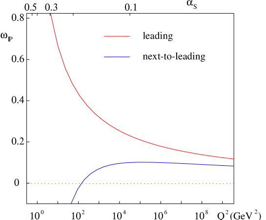
Figure 3.13: The BFKL hard pomeron $\omega_{\mathbb{P}}(\alpha_{\mathrm{s}})$ in leading and next-to-leading approximation.

As far as the perturbative factor is concerned, the integral representation (3.98) has an essential singularity at $\omega=0$. However, the anomalous dimension representation (3.99), depending on $\omega$ through $\bar{\gamma}_{\omega}$, is singular in correspondence of the branch cut $\omega_{\mathbb{P}}(\bar{\alpha}_{\mathrm{s}})$ of $\omega\mapsto\bar{\gamma}_{\omega}(\bar{\alpha}_{\mathrm{s}})$ given by

$$\omega_{\mathbb{P}}(\bar{\alpha}_{\mathrm{s}})\,\raisebox{0.37pt}{:}= \bar{\alpha}_{\mathrm{s}}\chi_{m}\simeq\bar{\alpha}_{\mathrm{s}}[\chi^{(0)}\big{(}{1\over 2}\big{)}+\bar{\alpha}_{\mathrm{s}}\chi^{(1)}\big{(}{1\over 2}\big{)}$$

$$= \omega_{\mathbb{P}}^{(\text{L}x)}(\bar{\alpha}_{\mathrm{s}})[1-6.47\bar{\alpha}_{\mathrm{s}}]\;.$$ (3.107)

Note that the value of $\omega_{\mathbb{P}}(\bar{\alpha}_{\mathrm{s}})$ is not affected by the choice of the energy-scale within the factorized class $s_{0}=k^{p}k_{0}^{1-p}$, since the shift $\Delta\chi^{(1)}(1/2)$ is proportional to $\chi^{(0)}{}^{\prime}(1/2)=0$ (cfr. Eq. (3.90)).

Due to the formal analogy of the definitions (3.107) and (2.73), $\omega_{\mathbb{P}}(\bar{\alpha}_{\mathrm{s}})$ is often called the hard pomeron singularity. To be fair, however, only the hard nature of $\omega_{\mathbb{P}}(\bar{\alpha}_{\mathrm{s}})$ is a fact. In fact we cannot guarantee it to be the rightmost singularity of the GGF. In addition, there may be sound doubts it to be a true singularity. In fact, $\omega_{\mathbb{P}}(\bar{\alpha}_{\mathrm{s}})$ signals the breakdown of the anomalous dimension representation (3.99) where the saddle point estimates does no more work.

Nevertheless, even if $\omega_{\mathbb{P}}(\bar{\alpha}_{\mathrm{s}})$ doesn’t correspond to a singular behaviour of ${\mathcal{G}}_{\omega}$, but rather to a singularity of the anomalous dimension, it may be related to a power-like behaviour in an intermediate small-$x$ moderate-$Q^{2}$ region. This assertion is confirmed by studies of some simplified models [43, 46] one of which we shall deal with in Chap. 5.

The last term in the RHS of Eq. (3.107) emphasizes the large and negative corrections stemming from the NL$x$ BFKL kernel. In Fig. 3.13 you can see that the maximum value of $\omega_{\mathbb{P}}(\bar{\alpha}_{\mathrm{s}})\simeq 0.11$ is reached for $\bar{\alpha}_{\mathrm{s}}\simeq 0.08$ and in the range of HERA data $Q^{2}\simeq 1\div 10^{4}\text{ GeV}^{2}$, i.e., $\bar{\alpha}_{\mathrm{s}}\simeq 0.1\div 0.4$, the NL$x$ hard pomeron is very small and even negative, in deep disagreement with the data (see Figs. 3.1).

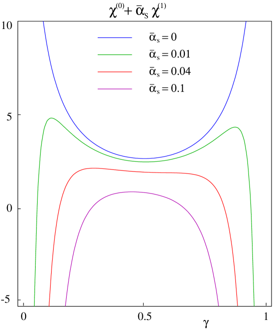
Figure 3.14: The BFKL eigenvalue function for different values of $\bar{\alpha}_{\mathrm{s}}$ and $N_{\!f}=0$. It is apparent the change in shape and the disappearance of the minimum for $\bar{\alpha}_{\mathrm{s}}>0.04$.

The situation is even worse if we look for the solution of Eq. (3.107) for finite (non vanishing) values of $\bar{\alpha}_{\mathrm{s}}$:

$$\omega_{\mathbb{P}}(\bar{\alpha}_{\mathrm{s}})=\underset{\gamma\in]0,1[}{\operatorname{{\rm Min}}}\bar{\alpha}_{\mathrm{s}}[\chi^{(0)}(\gamma)+\bar{\alpha}_{\mathrm{s}}\chi^{(1)}(\gamma)]\;.$$ (3.108)

The plot of the eigenvalue function in Fig. 3.14 shows that a stable minimum for $\chi$ exists only for very small values of $\bar{\alpha}_{\mathrm{s}}<0.04$, whereas for $\bar{\alpha}_{\mathrm{s}}>0.04$ the shape of $\chi$ is the opposite of the L$x$ eigenvalue. Among the physical consequences of this pathological behaviour there is the loss of positivity for the total cross section, as it was pointed out in Refs. [47, 48].

Does a reliable phenomenological analysis require the high energy $\ln 1/x$ resummation in NNL$x$ approximation? A simple arithmetic-geometric extrapolation based on the L$x$ and NL$x$ computation-time would suggest something like $20\div 100$ years of work. But it seems that the whole $\ln 1/x$ BFKL hierarchy has slow or even bad convergence problems. Rather than a 3-loops calculation it would be better to add some physical information, some consistency constraints with well established physics…

Chapter 4 Improvement of the small-$\boldsymbol{x}$ equation by RG analysis

After many years of calculations and expectations, the NL$x$ corrections to the kernel of the BFKL equation turned out to be so large as to question the very meaning of the high energy expansion (3.9), rising the compelling question of how to improve it.

Exact higher order calculations would be for sure a formidable task, both for their size and because they mix with unitarity effects [49] and thus cannot be described within the BFKL equation alone. Furthermore, there seems to be serious problems with the convergence of the kernel, as we will show in the next section.

The main issue is to understand the reasons of the pathological behaviour of the NL$x$ corrections. Just like for the problems concerning the subtraction of the leading terms from the reducible contributions of the NL$x$ kernel, the discussion of the large NL$x$ correction is fundamentally related to the issue of the choice of scales.

4.1 Origin of the double logarithms

In a high energy scattering process of two objects with transverse scales ${\boldsymbol{k}}^{2}$ and ${\boldsymbol{k}}_{0}^{2}$, the L$x$ BFKL equation resums all the leading logarithmic terms of the cross section of the form

$$\left(\bar{\alpha}_{\mathrm{s}}\,K^{(0)}\,\ln{s\over s_{0}}\right)\quad,\quad n\geqslant 0$$ (4.1)

and we have already remarked that, in L$x$ approximation, the choice of $s_{0}$ is immaterial.

In the NL$x$ approximation, the energy-scale is intimately connected to the form of the NL$x$ kernel (Sec. 3.5.2) and also to the structure of the GGF (Sec. 3.4). However, there is not a particular scale which seems to be preferable, rather there are various candidates according to the regime being investigated. We have already discussed the collinear-safe scale $s_{M}$ and the factorized Regge-motivated ones $kk_{0}$, $k^{2}$. Nevertheless, in the situation where $k^{2}\gg k_{0}^{2}$, the DGLAP approach (Chap. 1) tells us that each power of $\bar{\alpha}_{\mathrm{s}}$ is accompanied by a large $\ln k^{2}/k_{0}^{2}$ and that the correct scaling variable, carrying the whole $s$-dependence, is given by $x\simeq k^{2}/s$. In practice, the cross section has terms like

$${1\over k^{2}}\left(\bar{\alpha}_{\mathrm{s}}\,\ln{k^{2}\over k_{0}^{2}}\,\ln{s\over k^{2}}\right)\qquad(k^{2}\gg k_{0}^{2})\;.$$ (4.2)

Now, if we rewrite the general term (4.2) by adopting $kk_{0}$ as the scale of the energy, double logarithms ($\ln^{2}$) of the transverse momenta appear in the perturbative series:

$$(\ref{singlog})={1\over k^{2}}\sum_{m=0}^{n}{n\choose m}(-2)^{-m}\left(\bar{\alpha}_{\mathrm{s}}\ln^{2}{k^{2}\over k_{0}^{2}}\right)^{m}\left(\bar{\alpha}_{\mathrm{s}}\ln{s\over kk_{0}}\ln{k^{2}\over k_{0}^{2}}\right)^{n-m}\;.$$ (4.3)

For instance, the ${\mathcal{O}}(\bar{\alpha}_{\mathrm{s}}^{2})$ cross section at L$x$ level reads (see Eq. (3.54))

$${{\rm d}\sigma^{(2,\text{L}x)}_{\text{\sf a}\text{\sf b}}\over{\rm d}{\boldsymbol{k}}\,{\rm d}{\boldsymbol{k}}_{0}}=\bar{\alpha}_{\mathrm{s}}^{2}h_{\text{\sf a}}^{(0)}({\boldsymbol{k}})h_{\text{\sf b}}^{(0)}({\boldsymbol{k}}_{0})\ln^{2}{s\over s_{0}}K^{(0)}{}^{2}({\boldsymbol{k}},{\boldsymbol{k}}_{0})\;.$$ (4.4)

In the collinear limit ${\boldsymbol{k}}\gg{\boldsymbol{k}}_{0}$ we have $s_{0}=k^{2}$ and

$$K^{(0)}{}^{2}({\boldsymbol{k}},{\boldsymbol{k}}_{0}) \simeq\int{\rm d}{\boldsymbol{k}}^{\prime}\;{1\over\pi({\boldsymbol{k}}-{\boldsymbol{k}}^{\prime})^{2}}{1\over\pi({\boldsymbol{k}}^{\prime}-{\boldsymbol{k}}_{0})^{2}}$$

$$\simeq{1\over k^{2}}\left[\ln{k^{2}\over k_{0}^{2}}+{\mathcal{O}}(1)\right]\;,$$ (4.5)

which shows the single logarithmic term and, in Mellin $\gamma$-space, gives rise to a double pole $\bar{\alpha}_{\mathrm{s}}^{2}/\gamma^{2}$.

By shifting the energy-scale $s_{0}=k^{2}\to kk_{0}$, we get

$$K^{(0)}{}^{2}\ln^{2}{s\over k^{2}}\simeq{1\over k^{2}}\ln{k^{2}\over k_{0}^{2}}\ln^{2}{s\over k^{2}}\;\longrightarrow\;{1\over k^{2}}\ln{k^{2}\over k_{0}^{2}}\ln^{2}{s\over kk_{0}}-{1\over k^{2}}\ln^{2}{k^{2}\over k_{0}^{2}}\ln{s\over kk_{0}}+\text{NNL}x\;.$$ (4.6)

The L$x$ term, i.e., the coefficient of $\ln^{2}s$, remains unchanged whilst the NL$x$ term acquires the double logarithmic contribution $K^{(0)}\ln^{2}({k^{2}/k_{0}^{2}})$ whose eigenvalue gives rise to a cubic pole $\bar{\alpha}_{\mathrm{s}}^{2}/\gamma^{3}$.

In general, the appropriate DGLAP single logs corresponds to $\bar{\alpha}_{\mathrm{s}}^{n}/\gamma^{k}$ and $\bar{\alpha}_{\mathrm{s}}^{n}/(1-\gamma)^{k}$ poles with $k\leqslant n+1$. On the contrary, the presence of double logs involves poles with $n+1<k\leqslant 2n+1$.

We conclude with Salam [50] that the $\bar{\alpha}_{\mathrm{s}}$-expansion of the kernel in conjunction with a non collinear-safe energy scale, generate double logs, i.e., strong collinear singularities, in the lower order kernels.

4.2 A toy kernel

Now, with the aid of a toy model [50], we want to show that those strong collinear singularities are responsible of the instability of the finite order $\bar{\alpha}_{\mathrm{s}}\ln 1/x$ truncation. We can get an idea of that mechanism by considering the Lund model [51], consisting in a small-$x$ evolution equation for the unintegrated gluon density — derived in the context of the linked-dipole-chain (LCD) model — similar to the BFKL one but differing in the collinear region. The relevant equation can be written

$$\omega{\mathcal{F}}_{\omega}={\mathcal{F}}^{(0)}_{\omega}+{\mathcal{K}}_{\omega}{\mathcal{F}}_{\omega}\;,$$ (4.7)

where $\omega$ is the variable conjugate to $x=k^{2}/s$ — so that we are considering $s_{0}=k^{2}$ — and the kernel ${\mathcal{K}}_{\omega}$ admits the usual power-like eigenfunctions (2.59) and its eigenvalue is

$$\bar{\alpha}_{\mathrm{s}}\chi(\gamma,\omega)=\bar{\alpha}_{\mathrm{s}}[2\psi(1)-\psi(\gamma)-\psi(1-\gamma+\omega)]\;.$$ (4.8)

In complete analogy with the method of solution explained in the context of the BFKL equation, the anomalous dimension $\bar{\gamma}_{\omega}(\bar{\alpha}_{\mathrm{s}})$ is determined by the equation

$$\omega=\bar{\alpha}_{\mathrm{s}}\chi(\bar{\gamma},\omega)$$ (4.9)

or, equivalently,

$$\omega=\bar{\alpha}_{\mathrm{s}}\chi_{\text{eff}}(\bar{\gamma},\bar{\alpha}_{\mathrm{s}})\;,$$ (4.10)

where $\chi_{\text{eff}}(\gamma,\bar{\alpha}_{\mathrm{s}})$ is implicitly defined by the solution of Eq. (4.9) once $\gamma$ and $\bar{\alpha}_{\mathrm{s}}$ have been fixed.

In the DGLAP limit, corresponding to the region close to $\gamma=0$, the effective eigenvalue function has only simple poles $1/\gamma$ to all orders in $\bar{\alpha}_{\mathrm{s}}$:

$$\chi_{\text{eff}}(\gamma,\bar{\alpha}_{\mathrm{s}})={1\over\gamma}\;[1+{\mathcal{O}}(\bar{\alpha}_{\mathrm{s}})]+{\mathcal{O}}(\gamma^{0})\qquad(s_{0}=k^{2})\;.$$ (4.11)

In the opposite DGLAP limit, $k_{0}^{2}\gg k^{2}$, the relevant region of $\gamma$ is close to $\gamma=1$. Making the transformation to the relevant Bjorken scale $s_{0}=k_{0}^{2}$, using $\gamma\to\gamma+\omega$ (cfr. Secs. 3.5.3 and 4.3), there is only the pole $1/(1-\gamma)$:

$$\chi_{\text{eff}}(\gamma,\bar{\alpha}_{\mathrm{s}})={1\over 1-\gamma}\;[1+{\mathcal{O}}(\bar{\alpha}_{\mathrm{s}})]+{\mathcal{O}}\big{(}(1-\gamma)^{0}\big{)}\qquad(s_{0}=k_{0}^{2})\;.$$ (4.12)

So one is completely free of double transverse logarithms in both DGLAP limits.

In terms of the symmetric energy-scale $s_{0}=kk_{0}$, Eq. (4.8) becomes ($\gamma\to\gamma+\mbox{\small$\frac{1}{2}$}\omega$)

$$\chi(\gamma,\omega)=2\psi(1)-\psi(\gamma+\mbox{\small$\frac{1}{2}$}\omega)-\psi(1-\gamma+\mbox{\small$\frac{1}{2}$}\omega)\;.$$ (4.13)

The $\bar{\alpha}_{\mathrm{s}}$-expansion of the ensuing effective eigenvalue function

$$\chi_{\text{eff}}(\gamma,\bar{\alpha}_{\mathrm{s}}) =\sum_{n=0}^{\infty}\bar{\alpha}_{\mathrm{s}}^{n}\chi_{\text{eff}}^{(n)}(\gamma)\;,$$ (4.14a)

$$\chi_{\text{eff}}^{(0)}(\gamma) =2\psi(1)-\psi(\gamma)-\psi(1-\gamma)\;,$$ (4.14b)

$$\chi_{\text{eff}}^{(1)}(\gamma) =-{1\over 2}\chi_{\text{eff}}^{(0)}(\gamma)[\psi^{\prime}(\gamma)+\psi^{\prime}(1-\gamma)]\;,$$ (4.14c)

$$\chi_{\text{eff}}^{(2)}(\gamma) =-{1\over 2}\chi_{\text{eff}}^{(1)}(\gamma)[\psi^{\prime}(\gamma)+\psi^{\prime}(1-\gamma)]-{1\over 8}\chi_{\text{eff}}^{(0)}(\gamma)^{2}[\psi^{\prime\prime}(\gamma)+\psi^{\prime\prime}(1-\gamma)]\;,$$ (4.14d)

signals the presence of double logarithms from NL$x$ level on, as one can see from

$$\chi_{\text{eff}}^{(1)}(\gamma) =-{1\over 2\gamma^{3}}+{\mathcal{O}}\big{(}{1\over\gamma}\big{)}+\{\gamma\leftrightarrow 1-\gamma\}\;,$$ (4.15a)

$$\chi_{\text{eff}}^{(2)}(\gamma) =+{1\over 4\gamma^{5}}+{\mathcal{O}}\big{(}{1\over\gamma^{3}}\big{)}+\{\gamma\leftrightarrow 1-\gamma\}\;.$$ (4.15b)

Note that the most divergent part of $\chi_{\text{eff}}^{(1)}$ in the regions of $\gamma$ close to 0 and close to 1 is exactly the same of the NL$x$ BFKL eigenvalue (at scale $s_{0}=kk_{0}$)! Therefore, as previously remarked, the cubic poles of Eq. (3.79) are a consequence or the fact that the high-energy-factorization scale $kk_{0}$ is not collinear safe, i.e., is different from the Bjorken scale $k_{>}^{2}$.

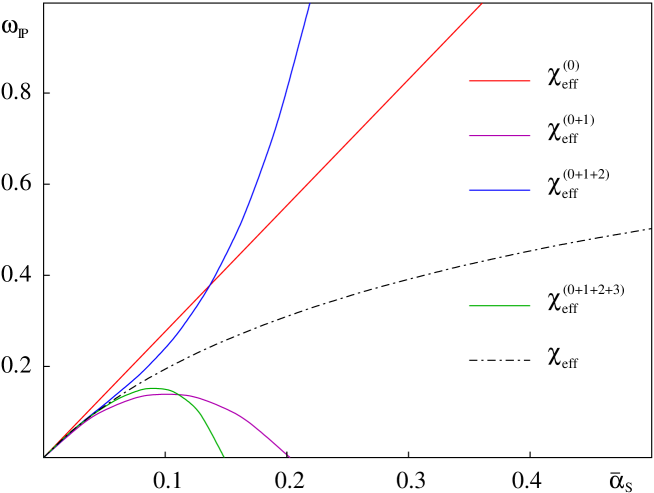
Figure 4.1: The toy-kernel pomeron singlularity as a function of $\bar{\alpha}_{\mathrm{s}}$, at leading, NL$x$, NNL$x$ , N³L$x$ and all orders.

If we look at the pomeron singularity $\omega_{\mathbb{P}}(\bar{\alpha}_{\mathrm{s}})=\bar{\alpha}_{\mathrm{s}}\chi_{\text{eff}}(1/2)$ of the toy-kernel in Fig. 4.1, we observe an alternate behaviour of the perturbative estimates, whose convergence is rather slow and limited to very low values of $\bar{\alpha}_{\mathrm{s}}$ in the lower approximations. For realistic values of $\bar{\alpha}_{\mathrm{s}}$, say 0.2, the fixed-order expansion are quite unreliable, and going from NL$x$ to NNL$x$ does not bring one any closer to the all-order result except for $\bar{\alpha}_{\mathrm{s}}\lesssim 0.1$.

To summarize, what one learns from this toy kernel is that the double transverse logarithms lead to a very poor convergence of the BFKL kernel at subleading orders and in particular the features of the analytic structure of the kernel and of the physical observables after the resummation are quite unrelated to the NL$x$ ones. Therefore, essential ingredients of any improvement of the BFKL approach should be the correct treatment of the collinear behaviour, as predicted by the RG, and the resummation of the corresponding collinear singularities to all orders.

4.3 Improved small-$\boldsymbol{x}$ kernel

In small-$x$ physics, Regge theory and the RG come to a sort of clash, which provides non trivial consistency requirements. The general form of the RG improved small-$x$ kernel is constrained by (i) the exact L$x$ and NL$x$ calculation and (ii) the collinear singulatity structure which we are going to specify. The latter requires to study the kernel in the collinear limits $k\gg k_{0}$ and $k\ll k_{0}$ where the relevant energy-scales are $k^{2}$ and $k_{0}^{2}$ respectively. It is also useful to consider the symmetric high-energy-factorization scale $kk_{0}$.

It is easy to see that, under energy-scale transformations of that kind, the GGF in Eq. (3.9) transforms according to

$$\overset{\text{\tiny s}}{{\mathcal{G}}}{}_{\omega}({\boldsymbol{k}},{\boldsymbol{k}}_{0})=\left({k_{0}\over k}\right)^{\omega}\overset{\text{\tiny u}}{{\mathcal{G}}}{}_{\omega}({\boldsymbol{k}},{\boldsymbol{k}}_{0})=\left({k\over k_{0}}\right)^{\omega}\overset{\text{\tiny l}}{{\mathcal{G}}}{}_{\omega}({\boldsymbol{k}},{\boldsymbol{k}}_{0})\;,$$ (4.16)

where the symmetric “$s$”, upper “$u$” and lower “$l$” suffixes refer to the energy-scales $kk_{0}$, $k^{2}$ and $k_{0}^{2}$. The similarity transformations (4.16) apply straightforwardly to the small-$x$ kernel defined by

$${\mathcal{G}}_{\omega}=[\omega-{\mathcal{K}}_{\omega}]^{-1}\;,$$ (4.17)

which we should consider $\omega$-dependent [52]:

$$\overset{\text{\tiny s}}{{\mathcal{K}}}_{\omega}({\boldsymbol{k}},{\boldsymbol{k}}_{0})=\left({k_{0}\over k}\right)^{\omega}\overset{\text{\tiny u}}{{\mathcal{K}}}_{\omega}({\boldsymbol{k}},{\boldsymbol{k}}_{0})=\left({k\over k_{0}}\right)^{\omega}\overset{\text{\tiny l}}{{\mathcal{K}}}_{\omega}({\boldsymbol{k}},{\boldsymbol{k}}_{0})\;.$$ (4.18)

Note that in the definition (4.17) of our improved small-$x$ kernel, the GGF does not contain any impact kernel.

We have already expressed the opinion that $\bar{\alpha}_{\mathrm{s}}$ is not a suitable expansion parameter for the kernel. The introduction of the $\omega$-dependence of ${\mathcal{K}}_{\omega}$ will reveal crucial in order to derive a novel small-$x$ expansion which automatically resums the collinear singularities.

From a perturbative point of view, however, we observe that, in general, the renormalized kernel ${\mathcal{K}}_{\omega}({\boldsymbol{k}},{\boldsymbol{k}}^{\prime};\mu^{2},\bar{\alpha}_{\mathrm{s}}(\mu^{2}))$ for non vanishing values of its arguments ${\boldsymbol{k}}$ and ${\boldsymbol{k}}^{\prime}$, is IR finite (see Secs. 2.3.1 and 3.5.3) and RG invariant, so that it can be expanded as a power series in $\bar{\alpha}_{\mathrm{s}}(k^{2})$ with scale-invariant coefficient kernels [52]

$${\mathcal{K}}_{\omega}({\boldsymbol{k}},{\boldsymbol{k}}^{\prime};\mu^{2},\bar{\alpha}_{\mathrm{s}}(\mu^{2}))=\sum_{n=0}^{\infty}\left[\bar{\alpha}_{\mathrm{s}}(k^{2})\right]^{n+1}K_{\omega}^{(n)}({\boldsymbol{k}},{\boldsymbol{k}}^{\prime})\;.$$ (4.19)

In other words, the only non scale-invariant source is the running coupling, which in Eq. (4.19) has been evaluated, for simplicity, at scale $k^{2}$. Different coupling-scales correspond to different, but always scale-invariant, coefficient kernels.

4.4 Form of the collinear singularities

We have shown in Sec. 3.6 (see also Refs. [45, 43]) that the BFKL equation satisfies RG factorization in an asymptotic way. The asymptotic form of the GGF for $t\,\raisebox{0.37pt}{:}=\ln k^{2}/\Lambda^{2}\gg t_{0}\,\raisebox{0.37pt}{:}=\ln k_{0}^{2}/\Lambda^{2}$ is given by

$$k^{2}\overset{\text{\tiny u}}{{\mathcal{G}}}{}_{\omega}({\boldsymbol{k}},{\boldsymbol{k}}_{0})\simeq C_{\omega}(\bar{\alpha}_{\mathrm{s}}(t))\Big{[}\exp\int_{t_{0}}^{t}\gamma^{+}_{\omega}(\bar{\alpha}_{\mathrm{s}}(\tau))\;{\rm d}\tau\Big{]}\widetilde{F}_{\omega}(t_{0})\;,$$ (4.20)

where $\gamma^{+}_{\omega}$ is the larger eigenvalue of the singlet anomalous dimension matrix, defined by the saddle point condition (3.100).

Therefore, the RG invariant kernel in the LHS of Eq. (4.19) acquires collinear singurarities for $k^{\prime}/k\to 0$ ($k/k^{\prime}\to 0$), which corresponds to strong ordering of the transverse momenta in the direction of the “upper” Bjorken scale $k^{2}$ (“lower” scale $k_{0}^{2}$). Such singularities are due to the non singular part $\tilde{\gamma}$ of the singlet anomalous dimension (3.106) which, neglecting the (small) $\text{\sf q}\bar{\text{\sf q}}$ contribution, is

$$\tilde{\gamma}_{\omega} =\gamma^{\text{\sf g}\text{\sf g}}_{\omega}-{\bar{\alpha}_{\mathrm{s}}\over\omega}=\bar{\alpha}_{\mathrm{s}}A_{1}(\omega)+\bar{\alpha}_{\mathrm{s}}^{2}A_{2}(\omega)+\cdots\;,$$ (4.21)

$$A_{1}(\omega) =-{11\over 12}+{\mathcal{O}}(\omega)\quad,\quad A_{2}(\omega)=0+{\mathcal{O}}(\omega)\;,$$

the singular part being taken into account by the BFKL iteration itself. It follows [52] that, for $k\gg k^{\prime}$,

$$\overset{\text{\tiny u}}{{\mathcal{K}}}_{\omega}({\boldsymbol{k}},{\boldsymbol{k}}^{\prime}) \simeq{\bar{\alpha}_{\mathrm{s}}(t)\over k^{2}}\;\exp\int_{t^{\prime}}^{t}\tilde{\gamma}_{\omega}(\alpha_{\mathrm{s}}(\tau))\;{\rm d}\tau\qquad(t\gg t^{\prime})$$ (4.22)

$$={\bar{\alpha}_{\mathrm{s}}(t)\over k^{2}}\left(1-b\bar{\alpha}_{\mathrm{s}}(t)\ln{k^{2}\over k^{\prime}{}^{2}}\right)^{-{A_{1}(\omega)\over b}}\;.$$

Expanding Eq. (4.22) in $\bar{\alpha}_{\mathrm{s}}(t)$ and comparing with the general definition (4.19), leads to the identification of the kernels $\overset{\text{\tiny u}}{K}{}_{\omega}^{(n)}$ in the collinear limit, whose eigenvalue functions turn out to have the singularities

$$\overset{\text{\tiny u}}{\chi}{}_{\omega}^{(n)}(\gamma)\simeq{1\cdot A_{1}(A_{1}+b)\cdots(A_{1}+(n-1)b)\over\gamma^{n+1}}\qquad(\gamma\ll 1)\;,$$ (4.23)

which correspond to single logarithmic scaling violations for $k\gg k_{0}$. A similar reasoning yields the collinear behavior of $\overset{\text{\tiny l}}{{\mathcal{K}}}_{\omega}$ in the opposite strong ordering region $k^{\prime}\gg k$

$$\overset{\text{\tiny l}}{{\mathcal{K}}}_{\omega}({\boldsymbol{k}},{\boldsymbol{k}}^{\prime}) \simeq{\bar{\alpha}_{\mathrm{s}}(t^{\prime})\over k^{\prime}{}^{2}}\;\exp\int_{t}^{t^{\prime}}\tilde{\gamma}_{\omega}(\alpha_{\mathrm{s}}(\tau))\;{\rm d}\tau\qquad(t^{\prime}\gg t)$$ (4.24)

$$={\bar{\alpha}_{\mathrm{s}}(t)\over k^{\prime}{}^{2}}\left(1-b\bar{\alpha}_{\mathrm{s}}(t)\ln{k^{\prime}{}^{2}\over k^{2}}\right)^{{A_{1}(\omega)\over b}-1}$$

and to the singularities

$$\overset{\text{\tiny l}}{\chi}{}_{\omega}^{(n)}(\gamma)\simeq{1\cdot(A_{1}-b)\cdots(A_{1}-nb)\over(1-\gamma)^{n+1}}\qquad(1-\gamma\ll 1)\;.$$ (4.25)

However, the similarity relations (4.18) connect the kernels $\overset{\text{\tiny u}}{{\mathcal{K}}}$ and $\overset{\text{\tiny l}}{{\mathcal{K}}}$. Therefore $\overset{\text{\tiny u}}{{\mathcal{K}}}$ has the singularities (4.25) shifted at $\gamma=1+\omega$ also, and similarly $\overset{\text{\tiny l}}{{\mathcal{K}}}$ has the singularities (4.23) shifted at $\gamma=-\omega$. As a consequence, the symmetric kernel $\overset{\text{\tiny s}}{{\mathcal{K}}}$ — for the energy-scale $s_{0}=kk_{0}$ — has both kinds of singularities shifted by $\pm\omega/2$:

$$\overset{\text{\tiny s}}{\chi}{}_{\omega}^{(n)}(\gamma) \simeq{1\cdot A_{1}(A_{1}+b)\cdots(A_{1}+(n-1)b)\over(\gamma+\mbox{\small$\frac{1}{2}$}\omega)^{n+1}}\qquad(\gamma\simeq-\mbox{\small$\frac{1}{2}$}\omega)\;,$$ (4.26a)

$$\simeq{1\cdot(A_{1}-b)(A_{1}-2b)\cdots(A_{1}-nb)\over(1-\gamma+\mbox{\small$\frac{1}{2}$}\omega)^{n+1}}\qquad(\gamma\simeq 1+\mbox{\small$\frac{1}{2}$}\omega)\;.$$ (4.26b)

Note the $b$-dependent asymmetry of the singularities in Eq. (4.26) under the $\gamma\leftrightarrow 1-\gamma$ transformation. It is due to the fact that the expansion (4.19) involves $\bar{\alpha}_{\mathrm{s}}(t)$ (and not $\bar{\alpha}_{\mathrm{s}}(t^{\prime})$). Of course, the kernel ${\mathcal{K}}_{\omega}$ itself must be symmetric under $t\leftrightarrow t^{\prime}$ exchange, so that expressing $\bar{\alpha}_{\mathrm{s}}(t^{\prime})$ in terms of $\bar{\alpha}_{\mathrm{s}}(t)$

$$\bar{\alpha}_{\mathrm{s}}(t^{\prime})={\bar{\alpha}_{\mathrm{s}}(t)\over 1-b\bar{\alpha}_{\mathrm{s}}(t)\ln\displaystyle{k^{2}\over k^{\prime}{}^{2}}}$$ (4.27)

leads to the symmetry constraints (in the following we omit the suffix “$s$”)

$$\chi_{\omega}^{(n)}(\gamma)=\sum_{m\leqslant n}{n\choose m}(-b\partial_{\gamma})^{n-m}\chi_{\omega}^{(m)}(1-\gamma)\;.$$ (4.28)

It is straightforward to check by the binomial identity

$${r+n\choose n}=\sum_{m=0}^{n}{r\choose m}{n\choose m}$$ (4.29)

that the symmetry constraints (4.28) are indeed satisfied by Eq. (4.26). In particular we must have

$$\chi_{\omega}^{(0)}(1-\gamma)=\chi_{\omega}^{(0)}(\gamma)\quad,\quad\chi_{\omega}^{(1)}(1-\gamma)=\chi_{\omega}^{(1)}(\gamma)+b\chi_{\omega}^{(0)}{}^{\prime}(\gamma)\;,$$ (4.30)

showing that the antisymmetric part of $\raisebox{1.5pt}{$\chi$}{}_{\omega}^{(1)}(\gamma)$ is $-{b\over 2}\raisebox{1.5pt}{$\chi$}{}_{\omega}^{(0)}{}^{\prime}(\gamma)$.

The coefficient kernels $K_{\omega}^{(n)}$ take up collinear singularities not only from the non singular part of the gluon anomalous dimension $\tilde{\gamma}^{\text{\sf g}\text{\sf g}}$, but also from $\text{\sf q}\bar{\text{\sf q}}$ states which are coupled to it in the one-loop gluon/quark-sea anomalous dimension matrix

$$\tilde{{\boldsymbol{\gamma}}}_{\omega}\,\raisebox{0.37pt}{:}={\boldsymbol{\gamma}}_{\omega}-{\bar{\alpha}_{\mathrm{s}}\over\omega}{0\quad 0\choose\textstyle{C_{F}\over C_{A}}\;1}=\bar{\alpha}_{\mathrm{s}}\boldsymbol{A}(\omega)\;.$$ (4.31)

Although the inclusion of the two-channel evolution (4.31) involves the collinear problem conceptually, the numerical effect of the quark-sea contribution to the gluon anomalous dimension is pretty small [44, 53]. Therefore, in the following, we will restrict our analysis to the gluon sector only.

4.4.1 Form of the leading coefficient kernel

Having determined the RG constraints, we are going to develop a procedure for defining the improved small-$x$ kernel at NL$x$ accuracy. The improved coefficient kernels $K_{\omega}^{(n)}$ are constructed by requiring that

• the Green’s function ${\mathcal{G}}_{\omega}$ reproduce the known NL$x$ calculations;

• the collinear singularities be as in Eq. (4.26).

In order to implement condition (1) we have first to relate the $\omega$-dependent formulation of ${\mathcal{G}}_{\omega}$ in Eq.(4.17) to the customary expression of the BFKL kernel at NL$x$ level

$${\mathcal{K}}=\bar{\alpha}_{\mathrm{s}}K^{(0)}+\bar{\alpha}_{\mathrm{s}}^{2}K^{(1)}+\cdots\;.$$ (4.32)

The $\omega$-dependent formulation of Eq. (4.19) yields instead the NL$x$ expansion

$${\mathcal{K}}_{\omega} =\bar{\alpha}_{\mathrm{s}}K_{0}^{(0)}+\bar{\alpha}_{\mathrm{s}}\omega K^{(0,1)}+\bar{\alpha}_{\mathrm{s}}^{2}K_{0}^{(1)}+\cdots\;,$$ (4.33)

$$K_{\omega}^{(n)}\,\raisebox{0.37pt}{:}=K_{0}^{(n)}+\omega K^{(n,1)}+\cdots\,,$$

which is actually more general than Eq. (4.32) because the $\bar{\alpha}_{\mathrm{s}}\omega$ term, coming from the $\omega$-expansion of $K_{\omega}^{(0)}$, is a possible NL$x$ contribution too.

Now it turns out that, at NL$x$ level, the formulation (4.33) reduces to the one in (4.32), provided the impact kernels $H_{L}$ and $H_{R}$ of Eq. (3.53) are taken into account [53]. In fact, by using the expansion (4.33) and simple operator identities, we can write

$$[\omega-{\mathcal{K}}_{\omega}]^{-1}=\left(1-\bar{\alpha}_{\mathrm{s}}K^{(0,1)}\right)^{-{1\over 2}}\left[\omega-(\bar{\alpha}_{\mathrm{s}}K^{(0)}+\bar{\alpha}_{\mathrm{s}}^{2}K^{(1)}+\cdots)\right]^{-1}\left(1-\bar{\alpha}_{\mathrm{s}}K^{(0,1)}\right)^{-{1\over 2}}$$ (4.34)

provided we set

$$K^{(0)} =K_{0}^{(0)}\;,$$ (4.35a)

$$K^{(1)} =K_{0}^{(1)}+K_{0}^{(0)}K^{(0,1)}\;.$$ (4.35b)

Eqs. (4.34) and (3.53) show that the two formulations above differ by just a redefinition of the impact kernels, while Eq. (4.35b) means that $K_{0}^{(1)}$ is given by $K^{(1)}$, after subtraction of the term already accounted for in the $\omega$-dependence of $K_{\omega}^{(0)}$.

The simplest way to define a L$x$ improved coefficient kernel fulfilling Eqs. (4.35a) and (4.26)$|_{n=0}$ is to displace the poles of $\raisebox{1.5pt}{$\chi$}{}^{(0)}_{\omega}$ in Eq. (3.80) by shifting the arguments of the $\psi$-functions, as suggested in Ref. [50]:

$$\chi_{\omega}^{(0)}(\gamma) =2\psi(1)-\psi(\gamma+\mbox{\small$\frac{1}{2}$}\omega)-\psi(1-\gamma+\mbox{\small$\frac{1}{2}$}\omega)$$ (4.36)

$$=\chi^{(0)}(\gamma)-{1\over 2}\omega{\pi^{2}\over\sin^{2}\pi\gamma}+\cdots\;.$$

The kernel $K_{\omega}^{(0)}$, corresponding to Eq. (4.36) is that occurring in the Lund model [51] and is given by

$$K_{\omega}^{(0)}({\boldsymbol{k}},{\boldsymbol{k}}^{\prime})=K^{(0)}({\boldsymbol{k}},{\boldsymbol{k}}^{\prime})\left({k_{<}\over k_{>}}\right)^{\omega}\;,$$ (4.37)

where $k_{>}\,\raisebox{0.37pt}{:}=\operatorname{{\rm Max}}(k,k^{\prime})$ and $k_{<}\,\raisebox{0.37pt}{:}=\operatorname{{\rm Min}}(k,k^{\prime})$. It is thus related to the customary leading kernel $K^{(0)}$ by the “threshold factor” $(k_{<}/k_{>})^{\omega}$. This means that the $s$-dependence provided by its inverse Mellin transform is [53]

$$K^{(0)}(s;{\boldsymbol{k}},{\boldsymbol{k}}^{\prime})\equiv\int{{\rm d}\omega\over 2\pi{\rm i}}\left({s\over kk^{\prime}}\right)^{\omega}{1\over\omega}K_{\omega}^{(0)}({\boldsymbol{k}},{\boldsymbol{k}}^{\prime})=K^{(0)}({\boldsymbol{k}},{\boldsymbol{k}}^{\prime})\,\Theta(s-k_{>}^{2})\;.$$ (4.38)

Can one justify the form of the kernel (4.37) “a priori”? From the point of view of the RG improved equation, any kernel which ($i$) reduces to $K^{(0)}$ in the $\omega\to 0$ limit and ($ii$) has the leading simple poles of Eq. (4.26) for $n=0$, is an acceptable starting point. An alternative choice of this kind will differ from $K_{\omega}^{(0)}$ by a NL$x$ kernel without $\gamma=0$ or $\gamma=1$ singularities. The resulting ambiguity can thus be reabsorbed by a proper subtraction in the NL$x$ coefficient kernel.

Nevertheless, the threshold interpretation of Eqs. (4.37) and (4.38) is appealing. For instance, the first iteration of such a kernel provides the expression

$$K^{(0)\,2}(s;{\boldsymbol{k}}_{1},{\boldsymbol{k}}_{2})= \int{{\rm d}\omega\over 2\pi{\rm i}}\left({s\over k_{1}k_{2}}\right)^{\omega}\left({1\over\omega}K_{\omega}^{(0)}\right)^{2}$$ (4.39)

$$= \int{\rm d}{\boldsymbol{k}}\;K^{(0)}({\boldsymbol{k}}_{1},{\boldsymbol{k}})\left(\ln{s\over k_{1}k_{2}}-\eta(k_{1},k)-\eta(k_{2},k)\right)K^{(0)}({\boldsymbol{k}},{\boldsymbol{k}}_{2})$$

where

$$\cosh\eta(k_{i},k)\equiv{k^{2}+k_{i}^{2}\over 2kk_{i}}\,.$$ (4.40)

The threshold condition implied by Eq. (4.39)

$${s\over 2k_{1}k_{2}}=\cosh\eta>\cosh\big{(}\eta(k_{1},k)+\eta(k,k_{2})\big{)}$$ (4.41)

is reminiscent of phase space in Toller variables [54] and may be regarded as an alternative way of stating coherence effects [30], as implied in the original version of the Lund model itself.

Whether or not such hints will eventually provide a more direct justification of $K_{\omega}^{(0)}$, the fact remains that Eq. (4.36) resums the $\omega$-dependence of the $\gamma$-singularities, and thus provides the correct singularities of the scale-dependent terms of the NL kernel. Therefore, it is a good starting point, yielding NL contributions which are smoother than those in the $\alpha_{\mathrm{s}}(t)$-expansion, as we now discuss.

4.4.2 Form of the next-to-leading contribution

The NL$x$ improved coefficient kernel is constrained by Eq. (4.26)$|_{n=1}$ and by Eq. (4.35b) which yields the $\omega=0$ limit of the eigenvalue function

$$\chi_{\omega=0}^{(1)}(\gamma)=\chi^{(1)}(\gamma)+{1\over 2}\chi^{(0)}(\gamma){\pi^{2}\over\sin^{2}\pi\gamma}\;.$$ (4.42)

The subtraction term so obtained is important because it has cubic poles at $\gamma=0,1$ which cancel the corresponding ones occurring in $\chi^{(1)}(\gamma)$. Furthermore, the impact kernels of Eq. (4.34) have quadratic poles which similarly account for the ones occurring in $H_{L}$ and $H_{R}$. This means that the remaining contributions are, in both cases, much smoother in the $\omega$-dependent formulation.

In order to implement condition (2) on $\raisebox{1.5pt}{$\chi$}{}_{\omega}^{(1)}$, we note that the $\omega=0$ limit (4.42) still contains double and single poles at $\gamma=0,1$, which should be shifted according to Eq. (4.26). By neglecting the (small) $\text{\sf q}\bar{\text{\sf q}}$ contributions, the explicit form of Eq. (4.42), following from Eq. (3.81) for the energy-scale $s_{0}=kk_{0}$, is [53]

$$\chi_{\omega=0}^{(1)}(\gamma)= -{1\over 2}\left({11\over 12}\big{(}\chi^{(0)\,2}(\gamma)+\chi^{(0)}{}^{\prime}(\gamma)\big{)}\right)+\left[-{1\over 4}\,\chi^{(0)}{}^{\prime\prime}(\gamma)+{1\over 2}\chi^{(0)}(\gamma){\pi^{2}\over\sin^{2}\pi\gamma}\right]+$$

$$-{1\over 4}\left\{\!\left({\pi\over\sin\pi\gamma}\right)^{2}\!\!{\cos\pi\gamma\over 3(1-2\gamma)}\left(11+{\gamma(1-\gamma)\over(1+2\gamma)(3-2\gamma)}\right)\right\}+$$

$$+\left({67\over 36}-{\pi^{2}\over 12}\right)\!\chi^{(0)}(\gamma)+{3\over 2}\,\zeta(3)+{\pi^{3}\over 4\sin\pi\gamma}-\Phi(\gamma)\;,$$ (4.43)

where $\Phi(\gamma)$ has been defined in Eq. (3.82). Here we have singled out some singular terms which have a natural physical interpretation, namely the running coupling terms (in round brackets), the energy-scale-dependent terms (in square brackets) and the collinear terms (in curly brackets).

The running coupling terms have a double pole at $\gamma=1$ only, and account for the asymmetric part of $\chi^{(1)}$ (given by $-{b\over 2}\chi^{(0)}{}^{\prime}$) which provides the $b$-dependent double pole on $\raisebox{1.5pt}{$\chi$}{}_{\omega}^{(1)}$ in Eq. (4.26). The collinear terms have symmetric double poles with residue $A_{1}(\omega=0)$, in accordance with Eq. (4.26) also. Both types of singularities can be shifted by adding a NNL$x$ term, vanishing in the $\omega=0$ limit, which we take to be

$$A_{1}(\omega)\psi^{\prime}(\gamma+\textstyle{\omega\over 2})-A_{1}(0)\psi^{\prime}(\gamma)+\big{(}A_{1}(\omega)-b\big{)}\psi^{\prime}(1-\gamma+\textstyle{\omega\over 2})-\big{(}A_{1}(0)-b\big{)}\psi^{\prime}(1-\gamma)\;.$$ (4.44)

This term incorporates the $\omega$-dependence of the one-loop anomalous dimension (4.21) too.

The energy-scale-dependent term in square brackets contains the subtraction (4.42) and has, therefore, simple poles at $\gamma=0,1$ only, which we can shift by adding the contribution

$${\pi^{2}\over 6}\big{(}\chi_{0}^{\omega}(\gamma)-\chi_{0}(\gamma)\big{)}\,.$$ (4.45)

By then collecting Eqs. (4.42), (4.44) and (4.45) we obtain the final eigenvalue function

$$\chi_{1}^{\omega}(\gamma)\equiv\tilde{\chi}_{1}(\gamma)+A_{1}(\omega)\psi^{\prime}(\gamma+\mbox{\small$\frac{1}{2}$}\omega)+\big{(}A_{1}(\omega)-b\big{)}\psi^{\prime}(1-\gamma+\mbox{\small$\frac{1}{2}$}\omega)+{\pi^{2}\over 6}\chi_{0}^{\omega}(\gamma)\;,$$ (4.46)

where

$$\tilde{\chi}^{(1)}(\gamma)\equiv\chi^{(1)}(\gamma)+{1\over 2}\chi^{(0)}(\gamma){\pi^{2}\over\sin^{2}\pi\gamma}-{\pi^{2}\over 6}\chi^{(0)}(\gamma)-A_{1}(0)\psi^{\prime}(\gamma)-\big{(}A_{1}(0)-b\big{)}\psi^{\prime}(1-\gamma)$$ (4.47)

is a symmetric function without $\gamma=0$ or $\gamma=1$ singularities at all. The expression (4.46) satisfies in addition the symmetry constraints (4.30), having antisymmetric part $-{b\over 2}\raisebox{1.5pt}{$\chi$}{}_{\omega}^{(0)}{}^{\prime}$.

Of course, there is some ambiguity involved in the choice of the subtraction terms (4.44, 4.45), which boils down to the possibility of adding to (4.47) a term, vanishing in the $\omega=0$ limit, and having only higher twist $\gamma$-singularities, around $\gamma=-1,-2,\cdots$ and $\gamma=2,3,\cdots$. We will discuss that ambiguity in Sec. 4.10.3.

4.4.3 Numerical importance of collinear effects at NLO

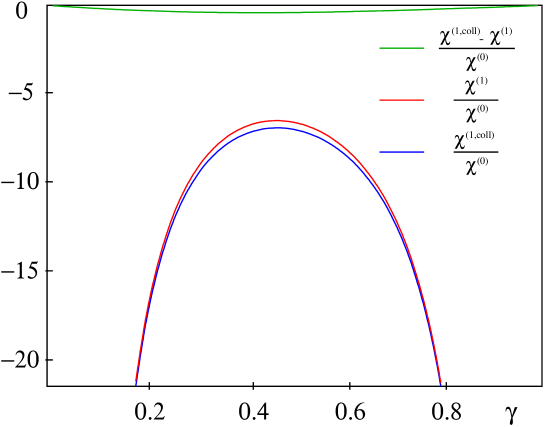
Figure 4.2: A comparison of the collinearly-enhanced (double and triple poles only) part of the NL$x$ corrections with the full NL$x$ corrections; $N_{\!f}=0$.

Above we have given the general form for the collinear singularities of the kernel at all orders. It is of interest to consider at NL$x$ level just how much of the full corrections come from these collinearly enhanced terms. Accordingly we look at the part of the NL$x$ corrections which contains just double and triple poles, $\chi^{(1)}_{\text{coll}}$:

$$\chi^{(1)}_{\text{coll}}=\frac{A_{1}}{\gamma^{2}}+\frac{A_{1}-b}{(1-\gamma)^{2}}-\frac{1}{2\gamma^{3}}-\frac{1}{2(1-\gamma)^{3}}\;.$$ (4.48)

This is compared with the full $\chi^{(1)}$ in Fig. 4.2, where we have plotted their ratios to $\chi^{(0)}$. The remarkable observation is that over a range of $\gamma$, the collinear approximation reproduces the true corrections to within $7\%$. It is obviously impossible to say whether this is true at higher orders as well. However the fact that the study of collinear terms has such predictive power at NL$x$ is a non-trivial point in favour of our resummation approach.

4.5 Factorization of non-perturbative effects

The next step is to obtain the improved GGF (4.17), i.e., to solve

$$\omega{\mathcal{G}}_{\omega}({\boldsymbol{k}},{\boldsymbol{k}}_{0})=\delta^{2}({\boldsymbol{k}}-{\boldsymbol{k}}_{0})+\int{\rm d}{\boldsymbol{k}}^{\prime}\;{\mathcal{K}}_{\omega}({\boldsymbol{k}},{\boldsymbol{k}}^{\prime}){\mathcal{G}}_{\omega}({\boldsymbol{k}}^{\prime},{\boldsymbol{k}}_{0})\;.$$ (4.49)

where an extention of the representation (4.19) in the region around the Landau pole $k^{2}\simeq\Lambda^{2}$ ($t=0$) is needed. However, for perturbation theory to be applicable, the non perturbative effects of such region should be factored out, as is predicted by the RG, and has been argued for at L$x$ and NL$x$ level [45, 43].

We assume that, by a suitable regularization of $\alpha_{\mathrm{s}}(t)$ around the Landau pole, ${\mathcal{K}}_{\omega}$ can be defined as a hermitian operator bounded from above in an ${\mathcal{L}}^{2}$ Hilbert space, with a continuum (or possibly discrete) spectrum $\text{Sp}({\mathcal{K}}_{\omega})\subset\;]-\infty,\mu_{\mathbb{P}}(\omega)]$. Typical regularizations of this kind may

• cut-off $\alpha_{\mathrm{s}}(t)$ below some value $t=\bar{t}>0$:

  $$\bar{\alpha}_{\mathrm{s}}(t)={1\over bt}\Theta(t-\bar{t})\;;$$ (4.50)

• freeze it in the form

  $$\bar{\alpha}_{\mathrm{s}}(t)={1\over bt}\Theta(t-\bar{t})+{1\over b\bar{t}}\Theta(\bar{t}-t)\;,$$ (4.51)

  possibly with some smoothing out around the cusp.

In such a framework, a formal solution for the Green’s function ${\mathcal{G}}_{\omega}$ is given by the spectral representation

$${\mathcal{G}}_{\omega}({\boldsymbol{k}},{\boldsymbol{k}}_{0})=\int_{-\infty}^{\mu_{\mathbb{P}}(\omega)}{{\rm d}\mu\over\pi}\;{F_{\omega}^{\mu}({\boldsymbol{k}})F_{\omega}^{\mu\,*}({\boldsymbol{k}}_{0})\over\omega-\mu}$$ (4.52)

in terms of a complete and orthonormal set of (real) eigenfunctions $F_{\omega}^{\mu}:\mu\in\text{Sp}({\mathcal{K}}_{\omega})$

$${\mathcal{K}}_{\omega}F_{\omega}^{\mu}=\mu F_{\omega}^{\mu}\;.$$ (4.53)

Let’s refer for definiteness to the frozen-$\bar{\alpha}_{\mathrm{s}}(t)$ regularization (4.51), which allows a simple classification of the eigenfunctions $F_{\omega}^{\mu}({\boldsymbol{k}})$ of Eq. (4.53), according to their behavior for $t\to-\infty$. In fact, since $\bar{\alpha}_{\mathrm{s}}(t)$ is fixed for $t<\bar{t}$, in the $t\to-\infty$ limit the eigenfunctions must behave just like the scale-invariant ones

$$(k^{2})^{\gamma(\mu)-1}={1\over k}{\rm e}^{{\rm i}\nu(\mu)t}\quad,\quad\gamma={1\over 2}+{\rm i}\nu\;.$$ (4.54)

Because of the symmetry property of the kernel with respect to the exchange of its arguments ${\boldsymbol{k}}\leftrightarrow{\boldsymbol{k}}^{\prime}$, to each eigenvalue $\mu$ there corresponds two opposite values $\pm\nu(\mu)$ and we can decompose the eigenfunctions $F_{\omega}^{\mu}({\boldsymbol{k}})$ as

$$F^{\mu}({\boldsymbol{k}}) \underset{\qquad\;}{=}\;{1\over 2{\rm i}}\left(E^{\nu(\mu)}({\boldsymbol{k}})-E^{-\nu(\mu)}({\boldsymbol{k}})\right)$$ (4.55)

$$\underset{t\to-\infty}{\simeq}\;{1\over 2{\rm i}k}\left(c(\nu){\rm e}^{{\rm i}\nu(\mu)t}-c^{*}(\nu){\rm e}^{-{\rm i}\nu(\mu)t}\right)$$

for suitable functions $E^{\nu}({\boldsymbol{k}})$ having a plane-wave asymptotic behavior for large and negative $t$ (the $\omega$ index has been dropped).

The precise superposition coefficient $c(\nu)$ of left- and right-moving waves occurring in Eq. (4.55) is determined by the condition that $F^{\mu}({\boldsymbol{k}})$ be regular for $t\to+\infty$, i.e., be vanishing at least as rapidly as $1/k$, so as to allow an ${\mathcal{L}}^{2}$ normalization.

If we assume $E^{\nu(\mu)}$ and $E^{-\nu(\mu)}$ to be boundary values of an imaginary analytic function $\widetilde{F}_{\omega}^{\mu}({\boldsymbol{k}})$ of $\mu$, whose branch cut lies along the spectrum (see Fig. 4.3), we can rewrite the spectral representation (4.52) as a contour integral

$${\mathcal{G}}_{\omega}({\boldsymbol{k}},{\boldsymbol{k}}_{0})=\int_{C(\omega)}{{\rm d}\mu\over 2\pi{\rm i}}\;{F_{\omega}^{\mu}({\boldsymbol{k}})\widetilde{F}_{\omega}^{\mu}({\boldsymbol{k}}_{0})\over\omega-\mu}\,,$$ (4.56)

encircling the spectrum $\text{Sp}({\mathcal{K}}_{\omega})$. By distorting the $\mu$-contour (because $\widetilde{F}^{\mu}$ is well behaved, for $\operatorname{\Re\text{e}}({\rm i}\nu)>0$) and by picking up the residue at the $\mu=\omega$ pole, we end up with the factorized expression [53]

$${\mathcal{G}}_{\omega}({\boldsymbol{k}},{\boldsymbol{k}}_{0})=F_{\omega}({\boldsymbol{k}})\widetilde{F}_{\omega}({\boldsymbol{k}}_{0})\qquad(k^{2}\gg k_{0}^{2})$$ (4.57)

where $F_{\omega}({\boldsymbol{k}})\,\raisebox{0.37pt}{:}=F_{\omega}^{\omega}({\boldsymbol{k}})$ and the same for $\widetilde{F}$. This procedure can be carried through provided $k/k_{0}$ is large enough for the decrease of $F^{\omega}$ to compensate the increase of $E^{\nu(\omega)}$.

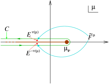
Figure 4.3: The function $\widetilde{F}^{\mu}$ is defined as that analytic function of $\mu$ whose limit on its branch cut — corresponding to the spectrum of ${\mathcal{K}}$ — is given by $E^{\nu(\mu)}$ ($E^{-\nu(\mu)}$) over (under) the cut. In this way the real integration in Eq. (4.52) can be replaced by a complex integration along the contour $C(\omega)$ of Eq. (4.56).

The plausibility argument above is further supported by the explicit model we will give in Chap. 5 for arbitrary values of $t$ and $t_{0}$, and hints at the general validity of Eq. (4.57). Therefore, for $k\gg k_{0}$, the Green’s function is asymptotically proportional — up to higher twist contributions — to the regular (for $t\to\infty$) solution $F_{\omega}({\boldsymbol{k}})$ of the homogeneous BFKL equation (4.53) with eigenvalue $\mu=\omega$:

$$\omega F_{\omega}={\mathcal{K}}_{\omega}F_{\omega}\;,$$ (4.58)

which becomes the basic quantity to be found.

4.6 The small-$\boldsymbol{\omega}$ expansion

Having determined the factorization property of the GGF in Eq. (4.57), we are now in a position to determine its perturbative (large-${\boldsymbol{k}}$) behaviour determined by the small-$x$ equation (4.58) whose kernel we know at NL$x$ level. In this section the scale of the energy $s_{0}$ is arbitrary, but one have to keep in mind that the resulting quantities depend on the scale chosen.

As usual it is better to work in $\gamma$-space, where we represent the eigenfunctions $F_{\omega}^{\mu}$ in a form hinted by Eq. (3.98):

$$F_{\omega}^{\mu}({\boldsymbol{k}})={1\over k}\int_{{1\over 2}-{\rm i}\infty}^{{1\over 2}+{\rm i}\infty}{{\rm d}\gamma\over 2\pi{\rm i}}\exp\left\{(\gamma-\mbox{\small$\frac{1}{2}$})t-{1\over b\mu}X_{\omega}(\gamma,\mu)\right\}\;,$$ (4.59)

where $X_{\omega}(\gamma,\mu)$ is to be found by solving Eq. (4.53).

By using the above representation for $F_{\omega}^{\mu}$ and keeping the general expression (4.19) for the kernel, the eigenvalue equation (4.53) becomes

$$0=[{\mathcal{K}}_{\omega}-\mu]F_{\omega}^{\mu}({\boldsymbol{k}})={1\over k}\int{{\rm d}\gamma\over 2\pi{\rm i}}\;{\rm e}^{(\gamma-\mbox{\small$\frac{1}{2}$})t-{1\over b\mu}X_{\omega}(\gamma,\mu)}\left[\sum_{n=0}^{\infty}\bar{\alpha}_{\mathrm{s}}(t)^{n+1}\chi_{\omega}^{(n)}(\gamma)-\mu\right]\;.$$ (4.60)

We assume that in the small-$\mu$, large-$t$ regime

$$bt\gtrsim{1\over\mu}\gtrsim{1\over\omega}\gg 1\;,$$ (4.61)

— resembling the anomalous dimension regime (3.101) — the integral (4.60) is dominated by a stable saddle point $\bar{\gamma}_{\omega}^{\mu}(\bar{\alpha}_{\mathrm{s}}(t))$ determined by the condition

$$\partial_{\gamma}\left\{(\gamma-\mbox{\small$\frac{1}{2}$})t-{1\over b\mu}X_{\omega}(\gamma,\mu)\right\}_{\gamma=\bar{\gamma}}=0\quad\iff\quad b\mu t=\partial_{\gamma}X_{\omega}^{\mu}(\bar{\gamma})\;,$$ (4.62a)

$$\partial_{\gamma}^{2}X_{\omega}(\bar{\gamma},\mu)<0\;.$$ (4.62b)

which need to be checked “a posteriori”.

By expanding in $\gamma$ the exponent and the eigenvalue functions $\raisebox{1.5pt}{$\chi$}{}_{\omega}^{(n)}$ around $\gamma=\bar{\gamma}$ and by keeping the ensuing fluctuations up to the relevant order, as explained in Ref. [53], Eq. (4.60) provides relations between the eigenvalues of the improved coefficient kernels and the $\gamma$-derivatives of $X_{\omega}(\gamma,\mu)$ which allows us to write the latter in terms of the former. More precisely, in the regime (4.61), we can express

$$\chi_{\omega}(\gamma,\mu)\,\raisebox{0.37pt}{:}=\partial_{\gamma}X_{\omega}(\gamma,\mu)\;,$$ (4.63)

by an expansion in $\mu$ whose coefficients are the eigenvalues $\raisebox{1.5pt}{$\chi$}{}_{\omega}^{(n)}$ and their $\gamma$-derivatives:

$$\chi_{\omega}(\gamma,\mu)=\eta_{\omega}^{(0)}(\gamma)+\mu\,\eta_{\omega}^{(1)}(\gamma)+\mu^{2}\,\eta_{\omega}^{(2)}(\gamma)+\cdots\;,$$ (4.64)

where the $\mu$-expansion coefficient $\eta_{\omega}^{(i)}$ could be derived, in principle, to all orders, and up to the third order (NNNL$x$) reads [53]

$$\eta_{\omega}^{(0)} =\chi_{\omega}^{(0)}\;,$$ (4.65a)

$$\eta_{\omega}^{(1)} ={\raisebox{1.5pt}{$\chi$}{}_{\omega}^{(1)}\over\raisebox{1.5pt}{$\chi$}{}_{\omega}^{(0)}}\;,$$ (4.65b)

$$\eta_{\omega}^{(2)} ={1\over\raisebox{1.5pt}{$\chi$}{}_{\omega}^{(0)}}\Bigg{[}{\raisebox{1.5pt}{$\chi$}{}_{\omega}^{(2)}\over\raisebox{1.5pt}{$\chi$}{}_{\omega}^{(0)}}+b\left({\raisebox{1.5pt}{$\chi$}{}_{\omega}^{(1)}\over\raisebox{1.5pt}{$\chi$}{}_{\omega}^{(0)}}\right)^{\prime}-\left({\raisebox{1.5pt}{$\chi$}{}_{\omega}^{(1)}\over\raisebox{1.5pt}{$\chi$}{}_{\omega}^{(0)}}\right)^{2}\Bigg{]}\;,$$ (4.65c)

$$\eta_{\omega}^{(3)} ={1\over\raisebox{1.5pt}{$\chi$}{}_{\omega}^{(0)}}\left[{\raisebox{1.5pt}{$\chi$}{}_{\omega}^{(3)}\over\raisebox{1.5pt}{$\chi$}{}_{\omega}^{(0)\,2}}+{b\over\raisebox{1.5pt}{$\chi$}{}_{\omega}^{(0)}}\left({\raisebox{1.5pt}{$\chi$}{}_{\omega}^{(2)}\over\raisebox{1.5pt}{$\chi$}{}_{\omega}^{(0)}}\right)^{\prime}-{\raisebox{1.5pt}{$\chi$}{}_{\omega}^{(1)}\raisebox{1.5pt}{$\chi$}{}_{\omega}^{(2)}\over\raisebox{1.5pt}{$\chi$}{}_{\omega}^{(0)\,3}}+b\,\eta_{\omega}^{(2)}{}^{\prime}-2\,\eta_{\omega}^{(1)}\eta_{\omega}^{(2)}\right]\;.$$ (4.65d)

In the $\mu=\omega$ case, Eq. (4.64) becomes an $\omega$-expansion [52] for

$$\chi_{\omega}(\gamma)\,\raisebox{0.37pt}{:}=\chi_{\omega}(\gamma,\omega)=\chi_{\omega}^{(0)}(\gamma)+\omega{\raisebox{1.5pt}{$\chi$}{}_{\omega}^{(1)}(\gamma)\over\raisebox{1.5pt}{$\chi$}{}_{\omega}^{(0)}(\gamma)}+\text{NNL}x\;,$$ (4.66)

which provides, through Eqs. (4.63), (4.59) and (4.57), the perturbative expression for the GGF we were looking for.

The analogy of Eqs. (4.62)$|_{\mu=\omega}\;\leftrightarrow\;$(3.100), (4.59)$\;\leftrightarrow\;$(3.98) and the L$x$ truncation of Eq. (4.66) leads to the identification of $\chi_{\omega}(\gamma)$ with the effective eigenvalue function of the improved kernel ${\mathcal{K}}_{\omega}$.

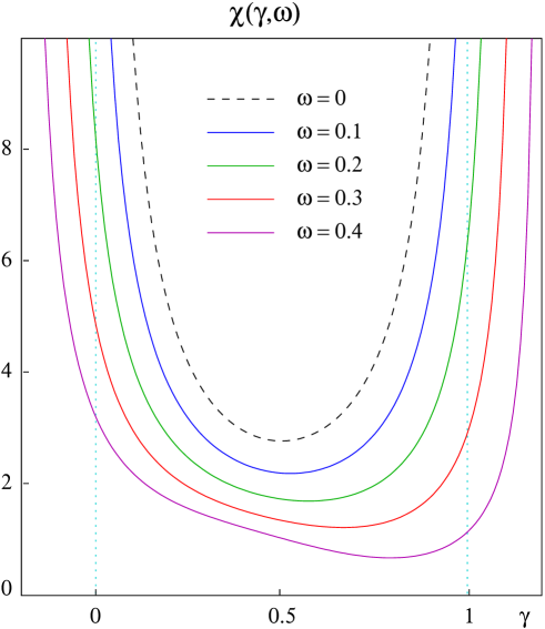
Figure 4.4: The NL$x$ truncation (4.66) of the effective eigenvalue function $\chi_{\omega}(\gamma)$; $N_{\!f}=0$.

Before entering the details of the determination of the improved anomalous dimension and of the hard pomeron, we would like to spend a few words about the major features of the improved eigenvalue $\raisebox{1.5pt}{$\chi$}{}_{\omega}(\gamma)$. In Fig. 4.4 you can see the effective eigenvalue function for various values of the new expansion parameter $\omega$. The stability of the shape, i.e., the presence of a minimum even for sizeable values of $\omega$ is apparent, at variance with Fig. 3.14. The shift of the poles is evident too, providing the consistency with the RG. The asymmetric shape is due to our (asymmetric) choice of the coupling-scale $k^{2}$.

4.7 Improved anomalous dimension

In order to study the anomalous dimension limit $Q^{2}\gg\Lambda^{2}$ of the integrated gluon density, let’s set the energy scale for the GGF to $s_{0}=k^{2}$. Due to the validity of RG factorization in the large-$t$ limit of Eq. (4.57), we can state that the gluon density $f^{(\text{\sf g}/H)}_{\omega}(Q^{2})$ in the hadron $H$ has a universal $t_{\!{}_{Q}}\,\raisebox{0.37pt}{:}=\ln Q^{2}/\Lambda^{2}$ dependence

$$f^{(\text{\sf g}/H)}_{\omega}(Q^{2})=g_{\omega}(t_{\!{}_{Q}})\,\tilde{g}_{\omega}^{(H)}\;,$$ (4.67)

where the $H$-dependent coefficient arise from Eq. (2.28)

$$\tilde{g}_{\omega}^{(H)}=\int{\rm d}{\boldsymbol{k}}_{0}\;\widetilde{F}_{\omega}({\boldsymbol{k}}_{0})\,f_{\omega}^{(\text{\sf g}/H)}({\boldsymbol{k}}_{0})$$ (4.68)

and is in general non perturbative, while the perturbative one is independent on the probe and is determined by

$$g_{\omega}(t_{\!{}_{Q}})=\int^{Q^{2}}{\rm d}{\boldsymbol{k}}\;F_{\omega}({\boldsymbol{k}})=\int{{\rm d}\gamma\over 2\pi{\rm i}}\;{1\over\gamma}\exp\left\{\gamma t_{\!{}_{Q}}-{1\over b\omega}\overset{u}{X}{}_{\omega}(\gamma)\right\}$$ (4.69)

where we have specified the function $X_{\omega}$ at the “upper” energy-scale $k^{2}$.

The asymptotic behaviour of Eq. (4.69) in the RG regime can be found from the saddle point (4.62) which, thanks to the identity

$$\bar{\gamma}_{\omega}t-X_{\omega}(\bar{\gamma})=\int^{t}\bar{\gamma}_{\omega}(\bar{\alpha}_{\mathrm{s}}(\tau))\;{\rm d}\tau+\text{const}$$ (4.70)

(check it by differentiating with respect to $t$) yields the result

$$g_{\omega}(t_{\!{}_{Q}})\simeq\left({1\over\bar{\gamma}_{\omega}}\sqrt{b\omega\over 2\pi|\overset{\text{\tiny u}}{\chi}{}_{\omega}^{\prime}(\bar{\gamma})|}+\cdots\right)\exp\int^{t_{\!{}_{Q}}}\bar{\gamma}_{\omega}(\bar{\alpha}_{\mathrm{s}}(\tau))\;{\rm d}\tau\;.$$ (4.71)

The coefficient in front, coming from the saddle point fluctuations, has been evaluated at NL level only. If we work at NL level, the saddle point approximation (4.71) is enough, and provides the effective anomalous dimension [53]

$$\gamma^{\text{eff}}_{\omega}(\bar{\alpha}_{\mathrm{s}}(t))\,\raisebox{0.37pt}{:}={{\rm d}\over{\rm d}t}\ln g_{\omega}(t) =\bar{\gamma}_{\omega}-{{\rm d}\over{\rm d}t}\ln\left[\bar{\gamma}_{\omega}\sqrt{|\overset{\text{\tiny u}}{\chi}{}_{\omega}^{\prime}(\bar{\gamma}_{\omega})|}\right]$$

$$=\bar{\gamma}_{\omega}-{b\omega\over\overset{\text{\tiny u}}{\chi}{}^{\prime}_{\omega}(\bar{\gamma}_{\omega})}\left({1\over\bar{\gamma}_{\omega}}+{\overset{\text{\tiny u}}{\chi}{}^{\prime\prime}_{\omega}(\bar{\gamma}_{\omega})\over 2\overset{\text{\tiny u}}{\chi}{}^{\prime}_{\omega}(\bar{\gamma}_{\omega})}\right)+\cdots$$ (4.72)

where in the last equality use have been made of the relation

$$b\omega t=\chi_{\omega}(\bar{\gamma}_{\omega})\quad\Longrightarrow\quad b\omega=\chi^{\prime}_{\omega}(\bar{\gamma}_{\omega}){{\rm d}\over{\rm d}t}\bar{\gamma}_{\omega}(\bar{\alpha}_{\mathrm{s}}(t))\;.$$ (4.73)

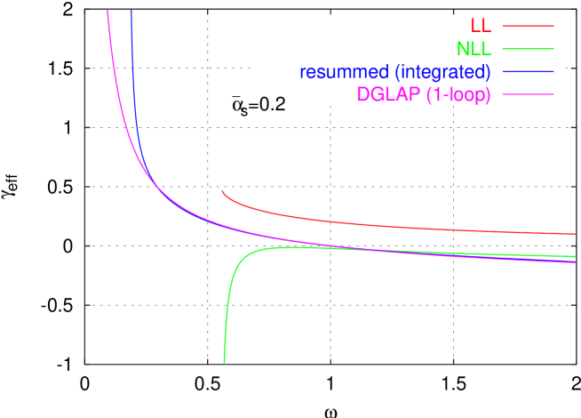
Figure 4.5: The anomalous dimension in various approximations.

Fig. 4.5 shows the (purely gluonic) anomalous dimension as a function of $\omega$ for $\bar{\alpha}_{\mathrm{s}}=0.2$. The L$x$ anomalous dimension is just $\gamma_{\textsc{l}}=\chi^{(0)\,-1}(\omega/\bar{\alpha}_{\mathrm{s}})$ and has the familiar branch-cut at $\omega=4\ln 2\bar{\alpha}_{\mathrm{s}}$. The NL$x$ anomalous dimension (3.105) has a divergent structure around the same point as $\gamma_{\textsc{l}}$. The resummed result, defined in Eqs. (4.69) and (4.72), shows a divergence at a much lower $\omega$, defined by $\omega_{c}(t)$, corresponding to the vanishing of the gluon density

$$g_{\omega_{c}(t)}(t)=0\;,$$ (4.74)

thus extending the resummed anomalous dimension beyond the spurious singularity of the BFKL truncation. What is particularly remarkable is the similarity to the DGLAP result until very close to the divergence. The momentum sum rule is automatically conserved: for $\omega=1$ we have $\gamma^{\text{eff}}_{1}=0$. Note however that, since $\omega_{c}(t)$ comes from a zero of $g_{\omega}(t)$, the $\omega=\omega_{c}(t)$ singularity does not transfer to $g_{\omega}(t)$ itself. Furthermore, the singularity of the anomalous dimension representation (4.71), coming from the failure of the saddle point expansion at the value $\omega=\omega_{s}(t)$ such that

$$\chi_{\omega_{s}}^{\prime}(\bar{\gamma}_{\omega_{s}}(t))=0\;,$$ (4.75)

is different from $\omega_{c}(t)$.

4.8 Improved hard pomeron

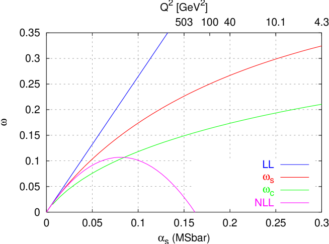
Figure 4.6: $\omega_{c}$ and $\omega_{s}$ as a function of $\alpha_{\mathrm{s}}$ for the BFKL kernel with $N_{\!f}=0$.

The values of the exponents $\omega_{c}$ and $\omega_{s}$ as a function of $\alpha_{\mathrm{s}}$ (and $Q^{2}$), are shown in Fig. 4.6 and compared with the L$x$ and pure NL$x$ results. It is apparent that the improved equation provides sensible predictions even for sizeable values of $\alpha_{\mathrm{s}}$. The above difference should not be too confusing. The exponent $\omega_{s}(t)$ signals the breakdown of the formal small-$x$ expansion of the anomalous dimension of Eq. (4.72), due to infinite saddle-point fluctuations, while $\omega_{c}(t)$ tells us the position of the singularity of the resummed anomalous dimension. Their difference arises from their different definitions, not from some instability of our approach.

What are the roles of the two hard pomeron estimates $\omega_{c}$ and $\omega_{s}$? What, if any, their relation to the pomeron singularity $\omega_{\mathbb{P}}$, the leading singularity of the GGF? We are not in a position to say a lot about those questions yet. Probably there is an intermediate small-$x$ moderate-$Q^{2}$ regime where the perturbative physics dominates, where $\omega_{c}$ or $\omega_{s}$ could be the effective small-$x$ growth exponent. The non perturbative soft pomeron, determined by the spectral condition $\omega_{\mathbb{P}}=\mu_{\mathbb{P}}(\omega_{\mathbb{P}})$, should however govern the very low-$x$ region.

In order to gain some hints on these issues, we have devised a simplified model [46] which allows one to treat in a semi-analytic way the whole $t$-space dependence and thus to estimete the (in)dependence of some physical quantities on the strong coupling region and also to clarify possible transition mechanisms between various $x$-regimes. But this is the subject of the last chapter.

4.9 Estimate of the NL$\boldsymbol{x}$ truncation error

What is the error that we make in the NL truncation of the RG improved equation? Our claim is that, in the improved formulation, based on the $\omega$-expansion (4.66), this error is smaller than in the formal NL expansion in $\alpha_{\mathrm{s}}(t)$. Let us in fact estimate the remaining terms in Eq. (4.64). According to Eq. (4.26) further subleading eigenvalue functions contain at least higher order collinear poles which contribute to $\eta_{\omega}^{(2)}$, $\eta_{\omega}^{(3)}$ and so on. A first observation is that, even if $\raisebox{1.5pt}{$\chi$}{}_{\omega}^{(n)}$ has ($n+1$)-th order poles, the $\eta_{\omega}^{(n)}:n\geqslant 0$ have at most simple poles, due to the powers of $\chi_{\omega}^{(0)}$ in the denominator, roughly due to the replacement $\bar{\alpha}_{\mathrm{s}}(t)\sim\omega/\raisebox{1.5pt}{$\chi$}{}_{\omega}^{(0)}$. Therefore, their contribution cannot be too big, even for small values of $\gamma={\mathcal{O}}(\omega)$.

Furthermore, one can check that, if $\text{\sf q}\bar{\text{\sf q}}$ contributions are neglected, the leading collinear poles actually cancel out in the expansions (4.65) of $\eta_{\omega}^{(2)}$, $\eta_{\omega}^{(3)}$, …around both $\gamma=0$ and $\gamma=1$. The mechanism of this cancellation is explained in Ref. [53].

From a physical point of view, it is not possible for simple poles to survive in $\eta_{\omega}^{(n)}:n\geqslant 2$, because, when replaced in the saddle point condition (4.73), they would provide $\omega^{n}:n\geqslant 2$ corrections to the 1-loop anomalous dimensions which cannot possibly be there. In fact, the full anomalous dimension is accounted for by Eqs. (4.66,4.62) as follows

$$b\omega t\simeq{1\over\bar{\gamma}_{\omega}}+{A_{1}(\omega)\over\bar{\gamma}_{\omega}}\quad\Longrightarrow\quad\bar{\gamma}_{\omega}=\bar{\alpha}_{\mathrm{s}}\left({1\over\omega}+A_{1}(\omega)\right)\;,$$ (4.76)

where we have taken the small-$\gamma$ limit of the collinear safe eigenvalue function $\overset{\text{\tiny u}}{\chi}{}_{\omega}(\gamma)$.

We therefore conclude that, in the purely gluonic case, the NL $\omega$-expansion (4.62) takes into account the collinear behavior to all-orders, and that no further resummation is needed.

4.10 Stability

The effective eigenvalue $\raisebox{1.5pt}{$\chi$}{}_{\omega}(\gamma)$ reveals its stability in shape providing a stable minimum and thus a reliable framework for small-$x$ physics. Nevertheless, there are some ambiguities, one of which is proper of the present resummation method and concerns the pole-shifting procedure of Sec. 4.4, others are typical of the perturbative treatments and concern the renormalization scheme prescription and the renormalization scale choice.

The original L$x$+NL$x$ formalism suffered from considerable instabilities under renormalization group scale and scheme changes [55]. An important characteristic of any resummed approach is that it should be relatively insensitive to such changes, and generally stable.

4.10.1 Renormalization scale

Note first that in our approach the renormalization scale only enters through the RG invariant $\Lambda$ parameter of $t=\ln k^{2}/\Lambda^{2}$ (Eqs. (4.19) and (4.69)). It is then easy to see that the physical results are $\Lambda$-independent. A redefinition of $\Lambda$ is essentially a shift in $t$, say by an amount $\Delta t$. There is a corresponding modification of $\chi_{\omega}^{(1)}$, $\chi_{\omega}^{(2)}$, …by the amounts

$$\chi_{\omega}^{(1)}\to\chi_{\omega}^{(1)}+b\Delta t\chi_{\omega}^{(0)}\quad,\quad\chi_{\omega}^{(2)}\to\chi_{\omega}^{(2)}+2b\Delta t\chi_{\omega}^{(1)}+b^{2}(\Delta t)^{2}\chi_{\omega}^{(0)}\quad,\quad\dots\;.$$ (4.77)

In the $\gamma$-representation (4.59), this corresponds to a modification of $X_{\omega}$ by an amount $b\mu\gamma\Delta t$. In fact the transformation (4.77) changes the coefficient $\eta^{(1)}_{\omega}$ only, the remaining ones $\eta^{(2)}_{\omega}$, $\eta^{(3)}_{\omega}$,…being left invariant. This change exactly cancels the modification of $t$ itself:

$$\exp\left\{\gamma t-{1\over b\mu}X_{\omega}(\gamma,\mu)\right\}\to\exp\left\{\gamma(t+\Delta t)-{1\over b\mu}(X_{\omega}(\gamma,\mu)+b\mu\gamma\Delta t)\right\}\;,$$ (4.78)

thus implying that the physical results are independent of the $\Lambda$-parameter choice [53]. This automatic resummation of the renormalization scale alleviates the need for techniques such as BLM resummation [56], advocated for example in [55], which show a strong renormalization scheme dependence.

4.10.2 Renormalization scale

The issue of renormalization scheme dependence is in fact closely related. Consider a scheme $S$ related to the $\overline{MS}$ scheme by

$$\alpha_{\mathrm{s}}^{(S)}=\alpha_{\mathrm{s}}^{(\overline{\text{\scriptsize MS}})}+T\alpha_{\mathrm{s}}^{2}\,,$$ (4.79)

with an appropriate modification of $\chi_{\omega}^{(1)}$. Except for terms of ${\mathcal{O}}(\alpha_{\mathrm{s}}^{3})$ and higher, this is identical to a renormalization scale change. Indeed if one defines the scheme change by a modification of $\Lambda$ then renormalization scheme changes behave exactly as renormalization scale changes, and so have no effect on the answer. Using instead 4.79 there is some residual dependence on the scheme at ${\mathcal{O}}(\alpha_{\mathrm{s}}^{3})$, but as one can see in Fig. 4.7 for the $\Upsilon$ scheme, which has $T\simeq 1.17$ (for $N_{\!f}=0$), the effect of the change of scheme is small.

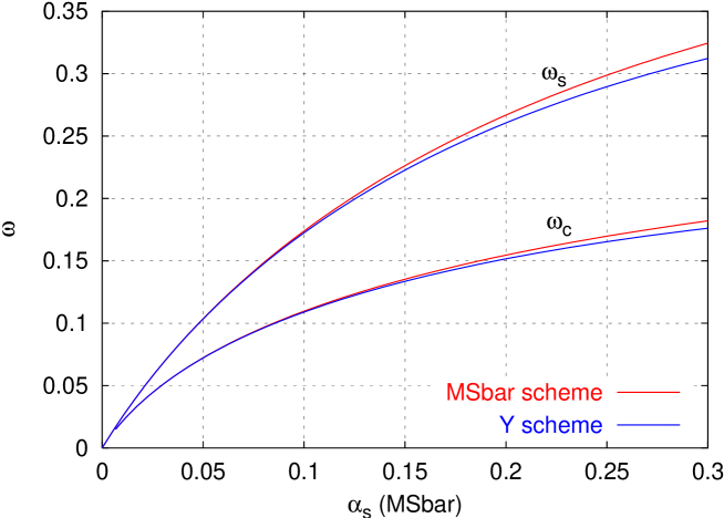
Figure 4.7: Renormalization scheme uncertainty of the two exponents; $\overline{MS}$ scheme and $\Upsilon$ scheme; $\alpha_{\mathrm{s}}$ is always shown in the $\overline{MS}$ scheme, and is connected to the $\Upsilon$ scheme value of $\alpha_{\mathrm{s}}$ via (4.79).

4.10.3 Resummation scheme

In resumming the double transverse logarithms (energy-scale terms), there is some freedom in one’s choice of how to shift the poles around $\gamma=0$ and $\gamma=1$. In a similar manner to what was done in [50] we consider two choices. The one explicitly discussed in this chapter can be summarized as

$$\psi^{(n-1)}(\gamma)\to\psi^{(n-1)}(\gamma+\mbox{\small$\frac{1}{2}$}\omega)\;,$$

with an equivalent procedure around $\gamma=1$. We refer to this as resummation scheme (a). An alternative possibility is (scheme (b))

$$\frac{1}{\gamma^{n}}\to\frac{1}{(\gamma+\mbox{\small$\frac{1}{2}$}\omega)^{n}}\;.$$

For instance, in this second scheme, the L$x$ improved eigenfunction would be

$$\chi^{(0)}_{\omega}(\gamma)=\chi^{(0)}(\gamma)-\frac{1}{\gamma}-\frac{1}{1-\gamma}+\frac{1}{\gamma+\mbox{\small$\frac{1}{2}$}\omega}+\frac{1}{1-\gamma+\mbox{\small$\frac{1}{2}$}\omega}\;.$$ (4.80)

A comparison of these two resummation schemes [53] is given in Fig. 4.8 and the difference between them is again reasonably small.

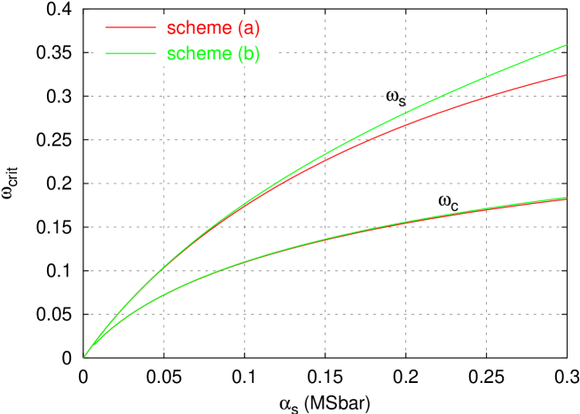
Figure 4.8: Resummation scheme uncertainty of the two critical exponents $\omega_{s}$ and $\omega_{c}$.

Aside from the explicit renormalization-scale independence, the stability of our approach is connected with the resummation of the collinear poles, for both the double-log, energy-scale dependent terms (the $1/\gamma^{3}$ and $1/(1-\gamma)^{3}$ poles at NL$x$ order) and for the single-log ones of Eq. (4.76).

Chapter 5 The collinear model

Let’s briefly review the results of the previous chapters. The study of perturbative high energy processes requires resummation techniques in order to correctly take into account the energy dependence. The BFKL approach provides such a framework, but exhibits an unstable behaviour as soon as the coupling exceeds very small values. It has been shown that the implementation of RG constrained collinear physics cures the BFKL hierarchy pathologies and the use of $\omega$ instead of $\alpha_{\mathrm{s}}$ as expansion parameter furnishes a stable framework where to study small-$x$ physics.

However, the improved formulation of Chap. 4 still leaves some open questions, concerning in particular the relative importance of perturbative versus non perturbative effects and the identification of the physical observables. Of course a lot of work has to be done yet in checking the validity of the factorization properties (4.57) of the GGF and on the novel small-$x$ equation (4.60) determining the perturbative solution.

For those purposes, we have devised a simple, but powerful tool for studying the problem of small-$x$ physics that we call the collinear model — namely a model where all and only the collinearly-enhanced physics is correctly included, in particular the full dependence on the one-loop running coupling, the splitting functions, and the so-called energy-scale terms (the ones in square brackets in Eq. (4.43). The model has the properties of correctly reproducing the one-loop renormalization group results and of being symmetric (given a problem with two transverse scales, its results do not depend on which of the scales is larger). These are properties desired from the resummation of the NLL corrections in the case of the full BFKL kernel.

While it does not correctly resum the series of leading and subleading logarithms of $s$ (i.e. the non-collinear part of the problem), in that region it does have a structure which qualitatively is very similar to that of the BFKL equation (cfr. Fig. 5.1) and can usefully serve as a model. In contrast to the BFKL equation, it is very easily soluble, as a Schrödinger-like problem.

5.1 Definition of the model

Our model [46] is defined in such a way to reproduce the DGLAP limits for branchings of gluons with ordered transverse momenta, and the anti-DGLAP limit for branchings with anti-ordered transverse momenta. In practice the kernel of this model extends the collinear asymptotic form (4.22) of the small-$x$ kernel down to $t\,\raisebox{0.37pt}{:}=\ln k^{2}/\Lambda^{2}\geqslant t^{\prime}\,\raisebox{0.37pt}{:}=\ln k^{\prime}{}^{2}/\Lambda^{2}$ while in the opposite region $t\leqslant t^{\prime}$ it is defined by Eq. (4.24). It is clear that the two expressions refer to the “upper” $k^{2}$ and “lower” $k_{0}^{2}$ energy-scales of the GGF respectively. By taking into account the energy-scale transformation relations (4.18) the symmetric expression of the collinear kernel reads

$${\mathcal{K}}_{\omega}(t,t^{\prime}) \,\raisebox{0.37pt}{:}=kk^{\prime}\overset{\text{\tiny s}}{{\mathcal{K}}}_{\omega}(k,k^{\prime})$$ (5.1)

$$=\bar{\alpha}_{\mathrm{s}}(t)\exp\left\{-{1+\omega\over 2}(t-t^{\prime})+A_{1}(\omega)\int_{t^{\prime}}^{t}\bar{\alpha}_{\mathrm{s}}(\tau)\,{\rm d}\tau\right\}\Theta(t-t^{\prime})+(t\leftrightarrow t^{\prime})\;,$$

$A_{1}(\omega)$ being the non singular part of the gluon anomalous dimension (4.21) at 1-loop.

Therefore the kernel for a single small-$x$ branching actually resums many branchings, of which the last (and only the last) is governed by the $1/\omega$ part of the splitting function and is taken into account in the iteration of the kernel giving the GGF

$${\mathcal{G}}_{\omega}={1\over\omega}\left[\boldsymbol{1}-{1\over\omega}{\mathcal{K}}_{\omega}\right]^{-1}$$ (5.2)

of the model.

The collinear properties of the kernel (5.1) can also be seen in $\gamma$-space, by the expansion

$${\mathcal{K}}_{\omega}(k,k^{\prime})=\sum_{n=0}^{\infty}[\bar{\alpha}_{\mathrm{s}}(k^{2})]^{n+1}\,K_{\omega}^{(n)}(k,k^{\prime})\;,$$

where the scale-invariant kernels $K_{\omega}^{(n)}$ have eigenvalue functions $\raisebox{1.5pt}{$\chi$}{}_{\omega}^{(n)}(\gamma)$ given by

$$\chi_{\omega}^{(n)}(\gamma)={1\cdot A_{1}(A_{1}+b)\cdots(A_{1}+(n-1)b)\over(\gamma+\textstyle{1\over 2}\omega)^{n+1}}+{1\cdot(A_{1}-b)(A_{1}-2b)\cdots(A_{1}-nb)\over(1-\gamma+\textstyle{1\over 2}\omega)^{n+1}}\;.$$ (5.3)

The leading order eigenvalue (cfr. Eq. (4.35a))

$$\chi^{(0)}(\gamma)\,\raisebox{0.37pt}{:}=\chi_{\omega=0}^{(0)}(\gamma)={1\over\gamma}+{1\over 1-\gamma}$$ (5.4)

differs from BFKL quite significantly numerically, but retains a very similar structure — a saddle point at $\gamma=1/2$ (see Fig. 5.1a), implying a power growth of the cross section, and diffusion.

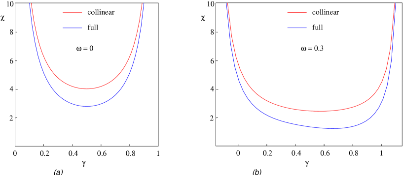
Figure 5.1: Comparison of the effective eigenvalue functions of the collinear model and of the full small-$x$ kernel of Chap. 4. In (a) the leading ($\omega=0$) ones and in (b) the L$x$+NL$x$ ones for $\omega=0.3$.

The NL$x$ eigenvalue (cfr. Eq. (4.35b))

$$\chi^{(1)}(\gamma)\,\raisebox{0.37pt}{:}=\chi^{(1)}_{\omega=0}(\gamma)+\chi^{(0)}_{\omega=0}\,\partial_{\omega}\chi^{(1)}_{\omega}|_{\omega=0}=\frac{A_{1}}{\gamma^{2}}+\frac{A_{1}-b}{(1-\gamma)^{2}}-\frac{\chi^{(0)}(\gamma)}{2}\left(\frac{1}{\gamma^{2}}+\frac{1}{(1-\gamma)^{2}}\right)$$ (5.5)

turns out to be very close, even numerically, to the full BFKL NLO kernel, reproducing it to better than $7\%$ over the whole range of $\gamma$ from $0$ to $1$ (cfr. Fig. 4.2). This confirms that collinearly enhanced effects dominate the NL$x$ kernel.

5.2 Differential equation formulations

5.2.1 First order formulation

The main advantage of our collinear kernel from the point of view of this article is its relative simplicity. Specifically it can be written in factorized form:

$${\mathcal{K}}_{\omega}(t,t^{\prime})=U_{\omega}(t)\,V_{\omega}(t^{\prime})\,\Theta(t-t^{\prime})+U_{\omega}(t^{\prime})\,V_{\omega}(t)\,\Theta(t^{\prime}-t)\,,$$ (5.6)

where (the $\omega$-dependence will be understood)

$$U(t) =\bar{\alpha}_{\mathrm{s}}(t)\exp\left\{-{1+\omega\over 2}t+A_{1}(\omega)\int^{t}\bar{\alpha}_{\mathrm{s}}(\tau)\,{\rm d}\tau\right\}\,,$$ (5.7a)

$$V(t) =\exp\left\{{1+\omega\over 2}t-A_{1}(\omega)\int^{t}\bar{\alpha}_{\mathrm{s}}(\tau)\,{\rm d}\tau\right\}\,.$$ (5.7b)

This allows us to recast the homogeneous BFKL equation

$$\omega{\mathcal{F}}(t)\equiv\omega k{\mathcal{F}}_{\omega}(k)=U(t)\int_{-\infty}^{t}{\rm d}t^{\prime}\;V(t^{\prime})\,{\mathcal{F}}(t^{\prime})+V(t)\int^{\infty}_{t}{\rm d}t^{\prime}\;U(t^{\prime})\,{\mathcal{F}}(t^{\prime})$$ (5.8)

as a differential equation. Dividing ${\mathcal{F}}$ into two parts,

$$\mathcal{A}(t) =U(t)\int_{-\infty}^{t}{\rm d}t^{\prime}\;V(t^{\prime})\,{\mathcal{F}}(t^{\prime})$$ (5.9a)

$$\mathcal{B}(t) =V(t)\int^{\infty}_{t}{\rm d}t^{\prime}\;U(t^{\prime})\,{\mathcal{F}}(t^{\prime})$$ (5.9b)

$$\omega{\mathcal{F}}(t) =\mathcal{A}(t)+\mathcal{B}(t)$$ (5.9c)

and taking the derivative leads to a pair of coupled differential equations:

$$\frac{{\rm d}\mathcal{A}}{{\rm d}t} =\frac{U^{\prime}}{U}\mathcal{A}+UV{\mathcal{F}}\,,$$ (5.10a)

$$\frac{{\rm d}\mathcal{B}}{{\rm d}t} =\frac{V^{\prime}}{V}\mathcal{B}-UV{\mathcal{F}}\,.$$ (5.10b)

For the specific kernel (5.1) that we consider, we have [46]

$$\frac{{\rm d}\mathcal{A}}{{\rm d}t} =\left(-\frac{1+\omega}{2}+A_{1}\bar{\alpha}_{\mathrm{s}}+\frac{\bar{\alpha}_{\mathrm{s}}^{\prime}}{\bar{\alpha}_{\mathrm{s}}}\right)\mathcal{A}+\bar{\alpha}_{\mathrm{s}}{\mathcal{F}}$$ (5.11a)

$$\frac{{\rm d}\mathcal{B}}{{\rm d}t} =\left(\frac{1+\omega}{2}-A_{1}\bar{\alpha}_{\mathrm{s}}\right)\mathcal{B}-\bar{\alpha}_{\mathrm{s}}{\mathcal{F}}$$ (5.11b)

Since we have two coupled equations, there are two independent solutions. Examining the equation for large and positive $t$, where $\bar{\alpha}_{\mathrm{s}}$ is small, one sees that they can be classified as a regular solution

$${\mathcal{F}}_{R}\sim\exp\left(-\frac{1+\omega}{2}t\right),$$ (5.12)

which is dominated by $\mathcal{A}$, and an irregular solution

$${\mathcal{F}}_{I}\sim\exp\left(\frac{1+\omega}{2}t\right),$$ (5.13)

dominated by $\mathcal{B}$.

5.2.2 Second order formulation

The coupled set of differential equations (5.10) can be recast in the form of a simple second order equation for ${\mathcal{F}}$. In fact, by using (5.9), we can first rewrite (5.10) in the form

$$\omega{\mathcal{F}}=\left[\left(\partial_{t}-\frac{U^{\prime}}{U}\right)^{-1}-\left(\partial_{t}-\frac{V^{\prime}}{V}\right)^{-1}\right]UV{\mathcal{F}}\,.$$ (5.14)

Then, in order to eliminate the resolvents appearing in (5.14) we introduce the operator

$${\mathcal{D}}_{t} =\left(\partial_{t}+\frac{U^{\prime}}{U}-\frac{w^{\prime}}{w}\right)\left(\partial_{t}-\frac{U^{\prime}}{U}\right)=\left(\partial_{t}+\frac{V^{\prime}}{V}-\frac{w^{\prime}}{w}\right)\left(\partial_{t}-\frac{V^{\prime}}{V}\right)$$ (5.15)

$$=\partial^{2}-{w^{\prime}\over w}\;\partial+{U^{\prime}V^{\prime\prime}-U^{\prime\prime}V^{\prime}\over w}\;,$$

and the wronskian

$$w(t)=W[U,V]\equiv UV^{\prime}-U^{\prime}V=\bar{\alpha}_{\mathrm{s}}(t)\left(1+\omega-2A_{1}\bar{\alpha}_{\mathrm{s}}-\frac{\bar{\alpha}_{\mathrm{s}}^{\prime}}{\bar{\alpha}_{\mathrm{s}}}\right)\,.$$ (5.16)

By applying ${\mathcal{D}}_{t}$ to (5.14) we finally obtain [46]

$$\omega{\mathcal{D}}_{t}{\mathcal{F}}=\left(\frac{U^{\prime}}{U}-\frac{V^{\prime}}{V}\right)UV{\mathcal{F}}=-w(t){\mathcal{F}},$$ (5.17)

which is the second order formulation that we were looking for.

Eq. (5.17) can be recast in normal form by the similarity transformation

$${\mathcal{F}}(t)={\rm const}\cdot\sqrt{w(t)}\,f(t)\,,$$ (5.18)

which leads to a Schrödinger type equation,

$$(-\partial_{t}^{2}+V_{\text{eff}})\,f =0$$ (5.19a)

$$V_{\text{eff}} =\frac{1}{4}\left(\frac{w^{\prime}}{w}\right)^{2}-\frac{1}{2}\left(\frac{w^{\prime}}{w}\right)^{\prime}-\frac{w}{\omega}+\frac{U^{\prime\prime}V^{\prime}-V^{\prime\prime}U^{\prime}}{w}\;.$$ (5.19b)

Note that the above derivation is valid for any form of the running coupling $\bar{\alpha}_{\mathrm{s}}(t)$ which extrapolates the perturbative form $(bt)^{-1}$ into the strong coupling region around the Landau pole $t=0$.

In what follows we consider various regularizations of the Landau pole, in particular the cut-off and the frozen $\alpha_{\mathrm{s}}$ cases defined in Eqs. (4.50) and (4.51). It is obvious that such different regularizations will change the form of the potential (Fig. 5.2) and thus the boundary conditions on ${\mathcal{F}}$ (or $f$) coming from the strong coupling region. A similar Schrödinger formulation was found [43] for the (Airy) diffusion model [4, 45] with running coupling, with a potential which roughly corresponds to the bottom of the well in Fig. 5.2.

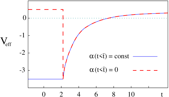
Figure 5.2: Qualitative $t$-dependence of the effective potential for the regularizations of type (a) and (b) of the coupling strength.

We consider in particular the solution ${\mathcal{F}}_{R}(t)$ (${\mathcal{F}}_{L}(t)$) of the homogeneous equation (5.17) which is regular for $t\to+\infty$ ($t\to-\infty$). If both conditions are satisfied, ${\mathcal{F}}_{R}={\mathcal{F}}_{L}$ is an eigenfunction of the BFKL equation. The pomeron singularity $\omega=\omega_{\mathbb{P}}$ is the maximum value of $\omega$ for which this occurs (ground state).

If $\omega>\omega_{\mathbb{P}}$, ${\mathcal{F}}_{R}\neq{\mathcal{F}}_{L}$ and the two solutions have rather different features. Due to the locality of the differential equation, ${\mathcal{F}}_{R}$ is independent of the regularization in the region $t>\bar{t}$. On the other hand, ${\mathcal{F}}_{L}$ will be dependent on the behaviour of $\bar{\alpha}_{\mathrm{s}}(t)$ for $t<\bar{t}$. For instance, in the case of $\bar{\alpha}_{\mathrm{s}}(t)$ being frozen (4.51), ${\mathcal{F}}_{L}$ has the exponential behaviour

$${\mathcal{F}}_{L}(t)\sim{\rm e}^{\kappa t}\,,\qquad(t<\bar{t})\,,$$ (5.20)

where $\kappa=\sqrt{V_{\text{eff}}(t<\bar{t})}$ is found from (5.19b) to be

$$\kappa^{2}=\left[\frac{1}{2}(1+\omega)-A_{1}\bar{\alpha}_{\mathrm{s}}(\bar{t})\right]\left[\frac{1}{2}(1+\omega)-A_{1}\bar{\alpha}_{\mathrm{s}}(\bar{t})-\frac{2\bar{\alpha}_{\mathrm{s}}(\bar{t})}{\omega}\right].$$ (5.21)

5.2.3 Factorization of non-perturbative effects

The basic tool for describing BFKL evolution is the Green’s function ${\mathcal{G}}_{\omega}(t,t_{0})\equiv kk_{0}{\mathcal{G}}_{\omega}(k,k_{0})$, which satisfies the inhomogeneous small-$x$ equation

$$\omega{\mathcal{G}}_{\omega}(t,t_{0})=\delta(t-t_{0})+{\mathcal{K}}_{\omega}\otimes{\mathcal{G}}_{\omega}(t,t_{0}),$$ (5.22)

and is supposed to be well-behaved for $t,t_{0}\to\pm\infty$. The problem of factorization is the question of the (in)dependence on the non-perturbative strong-coupling region.

For $t\neq t_{0}$, ${\mathcal{G}}_{\omega}$ satisfies the same differential equation as ${\mathcal{F}}$ and is thus a superposition of two independent solutions. The large-$t$ behaviour implies a regularity condition and suggests the expression

$${\mathcal{G}}_{\omega}(t,t_{0})={\mathcal{F}}_{R}(t){\mathcal{F}}_{L}(t_{0})\Theta(t-t_{0})+{\mathcal{F}}_{L}(t){\mathcal{F}}_{R}(t_{0})\Theta(t_{0}-t)\quad,\quad(t\neq t_{0})$$ (5.23)

Actually (5.23) is a rigorous consequence of the second-order formulation. In fact, ${\mathcal{G}}_{\omega}$ satisfies the differential equation

$$\left({\mathcal{D}}_{t}+{w\over\omega}\right){\mathcal{G}}_{\omega}={1\over\omega}{\mathcal{D}}_{t}\delta(t-t_{0})\,.$$ (5.24)

With a little thought, one can realize that ${\mathcal{G}}_{\omega}$ must contain a delta function term in the form

$${\mathcal{G}}_{\omega}(t,t_{0})={1\over\omega}\delta(t-t_{0})+\hat{{\mathcal{G}}}_{\omega}(t,t_{0})$$ (5.25)

and hence

$$\left({\mathcal{D}}_{t}+{w\over\omega}\right)\hat{{\mathcal{G}}}_{\omega}=-{w\over\omega^{2}}\delta(t-t_{0})$$ (5.26)

showing that $\hat{{\mathcal{G}}}$ is continuous function at $t=t_{0}$ with discontinuous derivative. Eq. (5.26) is an inhomogeneous Schrödinger type equation with a delta source, and its solution is just like the RHS of Eq. (5.23) also for $t=t_{0}$. We conclude that

$${\mathcal{G}}(t,t_{0})={1\over\omega}\delta(t-t_{0})+{\mathcal{F}}_{R}(t){\mathcal{F}}_{L}(t_{0})\Theta(t-t_{0})+{\mathcal{F}}_{L}(t){\mathcal{F}}_{R}(t_{0})\Theta(t_{0}-t)$$ (5.27)

with the normalization

$${\mathcal{F}}_{R,L}(t)=\frac{\sqrt{w(t)}}{\omega}f_{R,L}(t)\quad,\quad W[f_{R},f_{L}]\,\raisebox{0.37pt}{:}=f_{R}f^{\prime}_{L}-f_{R}^{\prime}f_{L}=1\,.$$ (5.28)

The main consequence of (5.23) is that the regularization dependence is factorized away in ${\mathcal{F}}_{L}$, whenever $t$ or $t_{0}$ are large enough. This happens in particular in the collinear limit $t-t_{0}\gg 1$ relevant for structure functions.

5.3 Solutions: analytical features

The collinear model just defined can be solved in principle as a Schrödinger problem by known analytical and numerical techniques and for both types of solutions occurring in the Green’s function (5.23) (i.e., the left-regular and the right-regular ones).

The right-regular solution ${\mathcal{F}}_{R}$ is, for large $t$, perturbative, i.e., independent of the potential in the strong coupling region $t\leqslant\bar{t}$, while the left-regular one ${\mathcal{F}}_{L}$ is dependent on the strong coupling. The left-regular solution ${\mathcal{F}}_{L}$ can be written as a superposition of the right-regular solution ${\mathcal{F}}_{R}$ and an other generic (linearly independent on ${\mathcal{F}}_{R}$) solution ${\mathcal{F}}_{I}$ (which is necessarily right-irregular, i.e., ${\mathcal{F}}_{I}\to\infty$ for $t\to+\infty$). By normalizing ${\mathcal{F}}_{I}$ in such a way that

$$W[f_{R},f_{I}]=1\quad,\quad{\mathcal{F}}_{I}(t)=\raisebox{0.37pt}{:}\hskip 3.0pt{\sqrt{w(t)}\over\omega}\,f_{I}(t)\;,$$ (5.29)

we have

$${\mathcal{F}}_{L}(t)={\mathcal{F}}_{I}(t)+S(\omega){\mathcal{F}}_{R}(t)\;.$$ (5.30)

The coefficient $S(\omega)$ is formally found from the matching conditions of both sides of Eq. (5.30) and their first derivatives at $t=\bar{t}$:

$$S(\omega)={{\mathcal{F}}_{I}(\bar{t}^{+})\over{\mathcal{F}}_{R}(\bar{t}^{+})}\cdot{{\mathcal{L}}_{I}(\omega)-{\mathcal{L}}_{L}(\omega)\over{\mathcal{L}}_{L}(\omega)-{\mathcal{L}}_{R}(\omega)}\quad,\quad{\mathcal{L}}_{i}\,\raisebox{0.37pt}{:}={{\mathcal{F}}^{\prime}_{i}(\bar{t}^{+})\over{\mathcal{F}}_{i}(\bar{t}^{+})}\;.$$ (5.31)

The coefficient ${\mathcal{L}}_{L}$ is provided by the strong coupling boundary conditions. In the two cases of regularization that we are considering we have

$$\left.{\mathcal{L}}_{L}\right|_{\rm freezing}={\kappa}(\omega)$$ (5.32)

$$\left.{\mathcal{L}}_{L}\right|_{\rm cutoff}=\left[\left({1+\omega\over 2}-A_{1}\bar{\alpha}_{\mathrm{s}}(\bar{t})\right)\left(1-{\bar{\alpha}_{\mathrm{s}}(\bar{t})\over\omega(1+\omega)}\right)+{\bar{\alpha}_{\mathrm{s}}^{\prime}(\bar{t})\over\omega(1+\omega)}\right]\left(1+{\bar{\alpha}_{\mathrm{s}}(\bar{t})\over\omega(1+\omega)}\right)^{-1}\,,$$ (5.33)

where $\bar{\alpha}_{\mathrm{s}}(\bar{t})$ is the $t\to\bar{t}^{+}$ limit of $\bar{\alpha}_{\mathrm{s}}(t)$.

Let us remark that, while ${\mathcal{F}}_{I}$ and ${\mathcal{F}}_{R}$ are expected to have an essential singularity at $\omega=0$ only, (cfr. Sec. 5.7), the coefficient $S(\omega)$ displays the leading part of the $\omega$-spectrum in $\operatorname{\Re\text{e}}\omega>0$, and in particular the leading Pomeron singularity $\omega_{\mathbb{P}}$. In fact, if $\omega\to\omega_{0}\in\text{Sp}({\mathcal{K}}_{\omega})$, then ${\mathcal{F}}_{L}\to\text{const}\times{\mathcal{F}}_{R}$ and the normalization condition (5.29) can be satisfied only if $S(\omega)\to\infty$.

The soft pomeron $\omega_{\mathbb{P}}$ is the greatest $\omega$-singularity of $S(\omega)$ and in the frozen-$\alpha_{\mathrm{s}}$ regularization it corresponds to the endpoint of the continuous spectrum. In the cut-off case, we expect also a discrete component in the spectrum (since there is a potential well, see Fig. 5.2) with poles at $\omega$-values such that ${\mathcal{L}}_{L}(\omega)={\mathcal{L}}_{R}(\omega)$, both being analytic functions in $\operatorname{\Re\text{e}}\omega>0$. Mixed cases are also possible, depending on the detailed shape of the potential in the strong coupling region.

Eq. (5.30) allows us to rewrite the Green’s function for $t>t_{0}$ and $\omega>\omega_{\mathbb{P}}$ in terms of $S(\omega)$ in Eq. (5.31) as follows:

$${\mathcal{G}}_{\omega}(t,t_{0})={\mathcal{F}}_{R}(t)\left[{\mathcal{F}}_{I}(t_{0})+S(\omega){\mathcal{F}}_{R}(t_{0})\right]\,.$$ (5.34)

If both $t,t_{0}\gg 1$, but $t-t_{0}={\mathcal{O}}(1)$, Eq. (5.34) is dominated by the first term, the second being suppressed exponentially in $t_{0}$ because the regular solution is much smaller than the irregular one for $t_{0}\gg 1$. This term is, on the other hand, defined by boundary conditions for $t,t_{0}\to+\infty$ only, and is therefore independent of the strong coupling region. Its analytical and numerical form will be discussed in more detail in the following.

The second term in Eq. (5.34) carries the regularization dependence and contains the leading $\omega$-singularities, in particular $\omega_{\mathbb{P}}$ (Ref. [39]). In $Y\,\raisebox{0.37pt}{:}=\log(s/kk_{0})$ space, the sum in Eq. (5.34) defines two asymptotic regimes, as we shall see.

5.4 Strong-coupling features

Within the collinear model we can study the spectrum of ${\mathcal{K}}_{\omega}$, which provides the $\omega$-singularities of the Green’s function embodied in $S(\omega)$, and in turn determine the high-energy behaviour of the cross section.

The leading $\omega$-singularity is the Pomeron $\omega_{\mathbb{P}}$, i.e., the maximum $\omega$ value for which a zero energy bound state for the potential (5.19b) is present. The pomeron properties depends on the coupling regularization. For smooth and non negative couplings the effective potential is a regular function bounded from below and increasing with $\omega$ so that there exists a value of $\omega=\omega_{\mathbb{P}}>0$ such that for $\omega>\omega_{\mathbb{P}}$ there are no more zero energy solutions. This demonstrates that the spectrum of the collinear kernel is bounded from above ($\text{Sp}({\mathcal{K}}_{\omega})\subset\;]-\infty,\omega_{\mathbb{P}}]$) for any regularization ($\omega_{\mathbb{P}}$ depends however on the regularization!).

In the following, we consider the two cases of freezing (4.51) and cutting-off (4.50) $\bar{\alpha}_{\mathrm{s}}(t)$. The first case is fairly simple, because for $t<\bar{t}$ the effective potential is constant and at its minimum value. Therefore $\omega_{\mathbb{P}}$, the upper limit of the continuous spectrum, given by $V^{\text{eff}}_{\omega}(t<\bar{t})-0$, is determined by the condition

$$\omega_{\mathbb{P}}={4\bar{\alpha}_{\mathrm{s}}(\bar{t})\over 1+\omega_{\mathbb{P}}-2\bar{\alpha}_{\mathrm{s}}(\bar{t})A_{1}(\omega_{\mathbb{P}})}\;.$$ (5.35)

This is to be compared with the saddle point definition of the hard Pomeron (4.75) $\omega_{s}(\bar{t})$, which is obtained by minimizing the solution (as a function of $\gamma$) of

$$\omega_{s}=\bar{\alpha}_{\mathrm{s}}\left(\chi_{0}^{\omega_{s}}(\gamma)+\omega_{s}\frac{\chi_{1}^{\omega_{s}}}{\chi_{0}^{\omega_{s}}}\right)\,.$$ (5.36)

Taking the $b=0$ form for $\chi_{1}^{\omega}$ the minimum is at $\gamma=1/2$, and $\omega_{s}$ is given by

$$\omega_{s}=\frac{4\bar{\alpha}_{\mathrm{s}}}{1+\omega_{s}-2\bar{\alpha}_{\mathrm{s}}A_{1}}\,.$$ (5.37)

which is identical to the true $\omega_{\mathbb{P}}$.

The second critical exponent $\omega_{c}(t)$ introduced in Sec. 4.7, corresponds to the rightmost singularity of the anomalous dimension. In the collinear model the integrated gluon distribution can be defined as

$$g_{\omega}(t_{\!{}_{Q}})\,\raisebox{0.37pt}{:}=\int_{-\infty}^{t_{\!{}_{Q}}}{\rm d}t\;\exp\left\{{1+\omega\over 2}t+A_{1}\int_{t}^{t_{\!{}_{Q}}}\bar{\alpha}_{\mathrm{s}}(\tau)\;{\rm d}\tau\right\}{\mathcal{F}}_{\omega}(t)={\mathcal{A}(t)\over\bar{\alpha}_{\mathrm{s}}(t)}$$ (5.38)

because $g_{\omega}(t)$ can be shown to satisfy, in the collinear limit, the usual DGLAP equation with anomalous dimension $(1/\omega+A_{1})\bar{\alpha}_{\mathrm{s}}$. The singularity of the anomalous dimension (at energy scale $k^{2}$)

$$\gamma^{\text{eff}}_{\omega}\big{(}\bar{\alpha}_{\mathrm{s}}(t)\big{)}\,\raisebox{0.37pt}{:}={{\rm d}\over{\rm d}t}\ln g_{\omega}(t)$$ (5.39)

is at the point $\omega=\omega_{c}(t)$ where $g_{\omega}(t)$ goes to zero, i.e., where $\mathcal{A}(t)$ goes to zero.

It is easier to discuss $\omega_{c}(t)$ in the cut-off case, in which $\bar{\alpha}_{\mathrm{s}}(t)=0$ for $t<\bar{t}$. In this case (5.38) allows us to write

$$\omega{\mathcal{F}}(t)=\mathcal{A}(t)+\mathcal{B}(t)=\bar{\alpha}_{\mathrm{s}}(t)g(t)+\mathcal{B}(t)\;.$$ (5.40)

By substituting (5.40) in the first order differential equation (5.11) it is not difficult to show that both $g(t)$ and $\mathcal{B}(t)$ are continuous at $t=\bar{t}$ and exponentially behaved for $t<\bar{t}$: $g\sim\mathcal{B}\sim\exp\big{(}\mbox{\small$\frac{1}{2}$}(1+\omega)t\big{)}$. It follows that

$${\mathcal{A}(\bar{t}^{+})\over\bar{\alpha}_{\mathrm{s}}(\bar{t}^{+})}=g(\bar{t})={\mathcal{B}(\bar{t})\over\omega(1+\omega)}\;.$$ (5.41)

For $\omega=\omega_{\mathbb{P}}$, ${\mathcal{F}}_{\omega_{\mathbb{P}}}(t)$ corresponds to the ground state of the system and have no zeroes:

$$0\neq{\mathcal{F}}_{\omega_{\mathbb{P}}}(\bar{t}^{+})={1\over\omega_{\mathbb{P}}}\big{(}\mathcal{A}(\bar{t}^{+})+\mathcal{B}(\bar{t})\big{)}={1\over\omega_{\mathbb{P}}}\left[{\bar{\alpha}_{\mathrm{s}}(\bar{t}^{+})\over\omega_{\mathbb{P}}(1+\omega_{\mathbb{P}})}+1\right]\mathcal{B}(\bar{t})\;,$$ (5.42)

hence $\mathcal{B}(\bar{t})\neq 0$ and also $g_{\omega_{\mathbb{P}}}(\bar{t})\neq 0$. In order to have $\mathcal{A}(\bar{t}^{+})=0$ one has to increase the depth of the potential well, i.e., to lower $\omega<\omega_{\mathbb{P}}$. This means that $\omega_{c}(\bar{t})<\omega_{\mathbb{P}}$.

The relationships just found ($\omega_{\mathbb{P}}^{\rm freezing}=\omega_{s}(\bar{t}),\;\omega_{\mathbb{P}}^{\rm cutoff}>\omega_{c}(\bar{t})$) represent two extreme cases of the boundary condition dependence of $\omega_{\mathbb{P}}$. If the coupling $\bar{\alpha}_{\mathrm{s}}(t)>0$ is positive but has intermediate size and shape for $t<\bar{t}$, we expect in general that

$$\omega_{c}(\bar{t})<\omega_{\mathbb{P}}<\omega_{s}(\bar{t})\;.$$ (5.43)

5.5 Perturbative regime: $\!\boldsymbol{\omega}$-expansion and WKB limit

Approximate homogeneous solutions in the large-$t$ region can be found, as in the full small-$x$ equation of Chap. 4, by the method of the $\gamma$-representation (4.59) and $\omega$-expansion (4.66). The regular solution is approximated, for $\omega\ll 1$, by the expression:

$${\mathcal{F}}_{R}(t)\simeq\int{{\rm d}\gamma\over 2\pi{\rm i}}\;\exp\left[(\gamma-\mbox{\small$\frac{1}{2}$})t-\frac{X^{\omega}}{b\omega}\right]\,,$$ (5.44)

with

$$\partial_{\gamma}X^{\omega}\equiv\chi(\gamma,\omega)=\chi^{\omega}_{0}(\gamma)+\omega\frac{\chi^{\omega}_{0}(\gamma)}{\chi^{\omega}_{1}(\gamma)}+{\mathcal{O}}(\omega^{2})$$ (5.45)

where, for the collinear model,

$$\chi^{\omega}_{0}(\gamma) =\frac{1}{\gamma+\mbox{\small$\frac{1}{2}$}\omega}+\frac{1}{1-\gamma+\mbox{\small$\frac{1}{2}$}\omega},$$ (5.46a)

$$\chi^{\omega}_{1}(\gamma) =\frac{A_{1}}{(\gamma+\mbox{\small$\frac{1}{2}$}\omega)^{2}}+\frac{A_{1}-b}{(1-\gamma+\mbox{\small$\frac{1}{2}$}\omega)^{2}}.$$ (5.46b)

In Chap. 4 this representation was extensively studied, and shown to be a solution of the problem up to next-to-leading order in $\omega$ and to all orders for the collinear structure. But this was only guaranteed to work true for small values of $\omega$ (whereas for the continuation with the DGLAP anomalous dimensions it is useful to be able to access high $\omega$ as well). Also there was no way of determining the coefficient of any higher-order error introduced by the procedure. A comparison of this representation with the exact solution, as is possible in the collinear model, is therefore important (cfr. Sec. 5.6.1).

The expressions (5.44–5.46) can be further specialized in the large-$t$ limit, where (5.44) is dominated by a saddle point at $\gamma=\bar{\gamma}_{\omega}(t):b\omega t=\chi(\bar{\gamma},\omega)$ and yields

$${\mathcal{F}}_{R}(t)=\sqrt{b\omega\over 2\pi|\chi_{\omega}^{\prime}(\bar{\gamma})|}\exp\int^{t}\bar{\gamma}(\tau)\;{\rm d}\tau\;.$$ (5.47)

We can obtain the large-$t$ behaviour of the right-regular solution by means of the WKB approximation for solving the differential equation (5.19). In fact, on the basis of Eqs. (5.19) and (5.28), one can prove the asymptotic expansion

$${\mathcal{F}}_{R}(t)={1\over\omega}\sqrt{w(t)\over 2\,{\kappa}(t)}\exp\left\{-\int_{t_{\kappa}}^{t}{\kappa}(\tau)\,{\rm d}\tau\right\}\times\left[1+{\mathcal{O}}\big{(}{1\over t}\big{)}\right]\,,$$ (5.48)

where ${\kappa}(t)$ is defined in terms of the effective potential (5.19b) as

$${\kappa}^{2}(t)\equiv V_{\text{eff}}(t)=\frac{1}{2}\left(1+\omega-{2A_{1}-b\over bt}\right)\left[\frac{1}{2}\left(1+\omega-{2A_{1}-b\over bt}\right)-\frac{2}{b\omega t}\right]+{\mathcal{O}}\big{(}{1\over t^{2}}\big{)}$$ (5.49)

and $t_{\kappa}$ is the zero of the WKB momentum: ${\kappa}(t_{\kappa})=0$.

Eq. (5.47) and (5.49) are asymptotic representations of the same function and are related by

$$\bar{\gamma}=\frac{1}{2}\left(1+{1\over t}\right)-{\kappa}(t)+{\mathcal{O}}\big{(}{1\over t^{2}}\big{)}\;.$$ (5.50)

It is interesting to note that in the collinear model, because of the differential equation (5.19), the present method yields the irregular solution also, which is obtained by just changing the sign of the WKB momentum ${\kappa}(t)$, i.e.,

$${\mathcal{F}}_{I}(t)={1\over\omega}\sqrt{w(t)\over 2\,{\kappa}(t)}\exp\left\{+\int_{t_{\kappa}}^{t}{\kappa}(\tau)\,{\rm d}\tau\right\}\,.$$ (5.51)

This is useful for evaluating the Green’s function according to Eq. (5.34).

5.6 Test of the $\boldsymbol{\omega}$-expansion

5.6.1 Right-regular solution

The possibility of evaluating (at least numerically) the GGF of the collinear model to arbitrary precision, allows us to test the validity of the $\omega$-expansion approximation method introduced in Sec. 4.6 by comparing the exact right-regular solution of the differential equation (5.11), or equivalently (5.19), with the $\gamma$-representation (5.44) where $X_{\omega}(\gamma)$ is determined by the NL$x$ truncation of the $\omega$-expansion (5.45). Fig. 5.3 shows the exact and approximated function ${\mathcal{F}}_{R}(t)$ for $\omega=0.15$. One sees that for larger values of $t$, the $\omega$-expansion is in good agreement with the exact solution, while for smaller $t$, where the solutions oscillate the results from the $\omega$-expansion are slightly out of phase with the exact solution. In general we are interested in the behaviour to the right of the rightmost zero.

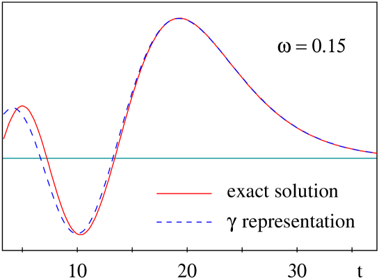
Figure 5.3: Right-regular solution from the explicit solution of the differential equation and from the $\omega$-expansion in arbitrary normalization; shown for $\omega=0.15$.

5.6.2 Critical exponent

One quantitative test of the $\omega$-expansion concerns the critical exponent $\omega_{c}$, i.e., the value of $\omega$ at which the effective anomalous dimension of Eq. (5.39) diverges. We recall that this is connected with the position of the rightmost zero of the regular solution: ${\mathcal{F}}_{\omega_{c}}(t)=0$. The $\omega$-expansion determination of the position of this zero, i.e., the zero of ${\mathcal{F}}_{R}(t)$ determined by means of the $\gamma$-representation (5.44) and the $\omega$-expansion (5.45), involves a small error which we call $\delta\omega_{c}$. Fig. 5.4 shows $\delta\omega_{c}/\omega_{c}$ as a function of $\omega_{c}$, and we see that the relative error on $\omega_{c}$ goes roughly as $\omega^{2}$, or equivalently as $\bar{\alpha}_{\mathrm{s}}^{2}$. This corresponds to a NNL$x$ correction and is beyond our level of approximation. We note also that even for relatively large values of $\omega\sim 0.3$, the relative correction remains of the order of $5\%$ which is quite acceptable. In other words the NNL$x$ correction that arises is not accompanied by a large coefficient.

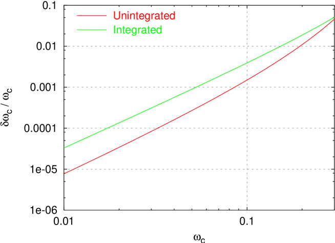
Figure 5.4: The error, $\delta\omega_{c}$ in the determination of $\omega_{c}$ within the $\omega$-expansion. Shown for both the unintegrated and integrated solutions.

5.6.3 Anomalous dimension

Our second quantitative test of the $\omega$-expansion concerns the anomalous dimension $\gamma_{\omega}$, as defined in Eq. (5.39). The error in the $\omega$-expansion result for the anomalous dimension, $\delta\gamma$, is plotted in Fig. 5.5 as a function of $\bar{\alpha}_{\mathrm{s}}$ for two values of $\omega$. Let us first concentrate on the region for $\bar{\alpha}_{\mathrm{s}}<0.01$. We see that the error is roughly independent of $\omega$, and proportional to $\bar{\alpha}_{\mathrm{s}}^{2}$. In other words the difference between the exact result and the $\omega$-expansion is a term of ${\mathcal{O}}(\bar{\alpha}_{\mathrm{s}}^{2})$. We recall that the terms that we wish to include properly are the leading terms $(\bar{\alpha}_{\mathrm{s}}/\omega)^{n}$, the NL terms $\bar{\alpha}_{\mathrm{s}}(\bar{\alpha}_{\mathrm{s}}/\omega)^{n}$ and the collinear terms $(\bar{\alpha}_{\mathrm{s}}/\omega)\omega^{n}$. A first correction of ${\mathcal{O}}(\bar{\alpha}_{\mathrm{s}}^{2})$ is consistent with all these terms having been correctly included.

For $\bar{\alpha}_{\mathrm{s}}>0.01$ we see that the error in the anomalous dimension has a more complicated behaviour: it changes sign (the dip) and then diverges, at the same point as the divergence in the anomalous dimension itself (solid curve): this is just a consequence of the position of the divergence of the anomalous dimension from the $\omega$-expansion being slightly different from the true position

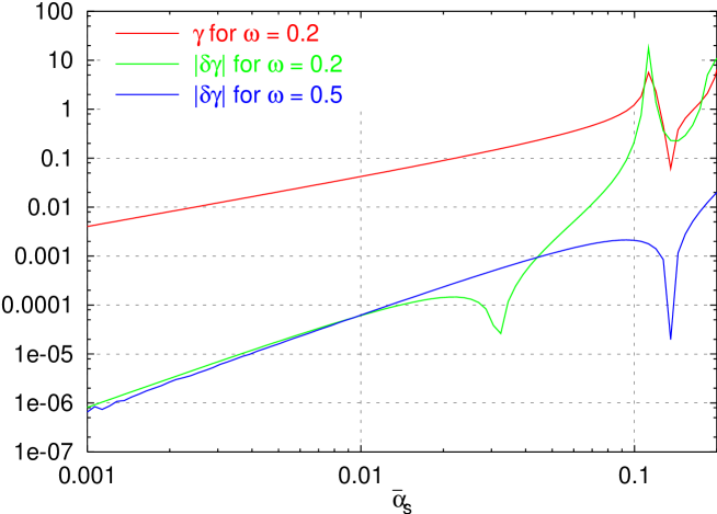
Figure 5.5: Error in the effective anomalous dimension of Eq. (5.39) from the $\omega$-expansion plotted against $\alpha_{\mathrm{s}}(t)$.

5.7 High energy behaviour

It is widely believed that a two-scale process — described by a small-$x$ equation of BFKL type — is perturbative for large enough $t$ and $t_{0}$, while it becomes a strong coupling process if the energy is so large as to allow diffusion to small values of $t\simeq 0$ ($k^{2}\simeq\Lambda^{2}$) [57, 58].

In the collinear model the Green’s function has the explicit expression (5.34), in which the strong-coupling information is clearly embodied in the reflection coefficient $S(\omega)$. Therefore it allows a direct study of the relative importance of the “perturbative” part ${\mathcal{F}}_{R}\otimes{\mathcal{F}}_{I}$ and of the “strong-coupling” part $S\,{\mathcal{F}}_{R}\otimes{\mathcal{F}}_{R}$, induced by diffusion through the boundary conditions at $t=\bar{t}$.

For large $t$ and $t_{0}$, the factorized form (5.23) of $\hat{{\mathcal{G}}}_{\omega}$ can be approximated by the WKB expression of Eq. (5.48,5.51), that we study in the special case $t=t_{0}$, so that the GGF in $Y\,\raisebox{0.37pt}{:}=\ln s/kk_{0}$ space is

$$\hat{{\mathcal{G}}}(Y;t,t)\simeq\int{{\rm d}\omega\over 2\pi{\rm i}}\;{\rm e}^{\omega Y}{w(t)\over 2\omega^{2}{\kappa}_{\omega}(t)}\left[1+S(\omega)\exp\left(-2\int_{t_{\kappa}}^{t}{\kappa}_{\omega}(\tau)\,{\rm d}\tau\right)\right]$$ (5.52)

for large enough $t$. The (perturbative) first term is characterized by a saddle point at $\omega=\bar{\omega}(t)>\omega_{s}(t)>0$ placed between the vertical asymptote of $1/{\kappa}_{\omega}(t)$ at $\omega\simeq\omega_{s}(t)$ on the left and the fast rising exponent ${\rm e}^{\omega Y}$ on the right. Since around $\omega_{s}$ we have ${\kappa}_{\omega}^{2}(t)\simeq\text{const}(t)\;[\omega-\omega_{s}(t)]$, the saddle point condition reads

$$\left.Y=\frac{1}{2}{\partial\over\partial\omega}\log{\kappa}^{2}_{\omega}\right|_{\omega=\bar{\omega}}\simeq{1\over 2(\bar{\omega}-\omega_{s})}\;,$$ (5.53)

hence

$$\bar{\omega}(Y,t)\simeq\omega_{s}(t)+{1\over 2Y}\;.$$ (5.54)

The saddle point (5.54) is self consistent provided the WKB approximation is valid, i.e., the variation of the WKB momentum ${\kappa}(t)$ is small on the typical wave-length of the solution:

$${\partial_{t}{\kappa}\over{\kappa}}\Big{/}{2\pi\over{\kappa}}\ll 1\quad\iff\quad 2Y\ll\left({2\over b}\right)^{2\over 3}\omega_{s}(t)^{-{5\over 3}}\sim\bar{\alpha}_{\mathrm{s}}(t)^{-{5\over 3}}$$ (5.55a)

and provided $$Y$$ is not too small so that the saddle point is not too shallow:

$${1\over 2Y}\ll\omega_{s}(t)\sim\bar{\alpha}_{\mathrm{s}}(t)\;.$$ (5.55b)

The saddle point estimate is finally performed by means of the integral

$$\int_{\epsilon-{\rm i}\infty}^{\epsilon+{\rm i}\infty}{{\rm d}x\over 2{\rm i}\sqrt{\pi x}}{\rm e}^{x}=1\,,\quad(x\equiv(\omega-\omega_{s})Y)$$ (5.56)

rather than by naïve quadratic fluctuations around $x=1/2$ and yields [46]

$$\hat{{\mathcal{G}}}^{(\text{pert})}(Y;t,t)\simeq{1\over\sqrt{2\pi\chi_{m}^{\prime\prime}\bar{\alpha}_{\mathrm{s}}Y}}\,{\rm e}^{\omega_{s}(t)Y}\times\left[1+{\mathcal{O}}(\alpha_{\mathrm{s}}^{5}Y^{3})\right]\quad,\quad\chi_{m}^{\prime\prime}(t)\,\raisebox{0.37pt}{:}=\underset{\gamma}{\operatorname{{\rm Min}}}\,\chi\big{(}\gamma,\omega_{s}(t)\big{)}\;.$$ (5.57)

The contribution of the (non perturbative) second term of Eq. (5.52) is evaluated with the residue method

$$\hat{{\mathcal{G}}}^{(\text{nopt})}(Y;t,t)=\sum_{\omega_{i}\in\{\text{poles}\}}{\rm e}^{\omega_{i}Y}R_{i}{\rm e}^{-2\int_{t_{\kappa}}^{t}{\kappa}_{\omega_{i}}(\tau)\,{\rm d}\tau}\;.$$ (5.58)

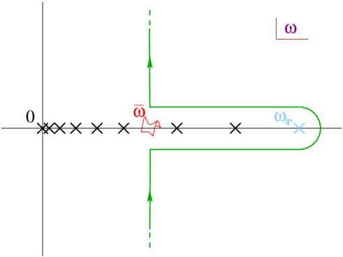
Figure 5.6: The contour of integration for the Green’s function $\hat{{\mathcal{G}}}_{\omega}(Y;t,t)$, displaying the pole contribution of the non perturbative part and the background integral parallel to the imaginary axis relevant for the perturbative part of the GGF.

Retaining only the leading pole $\omega_{\mathbb{P}}$ and observing that ${\kappa}_{\omega_{\mathbb{P}}}(\tau)\simeq(1+\omega_{\mathbb{P}})/2+{\mathcal{O}}(1/\tau)$, we end up with the result [46]

$$\hat{{\mathcal{G}}}(Y;t,t)\simeq{1\over\sqrt{2\pi\chi_{m}^{\prime\prime}\bar{\alpha}_{\mathrm{s}}Y}}\,{\rm e}^{\omega_{s}(t)Y}\times\left[1+{\mathcal{O}}(\alpha_{\mathrm{s}}^{5}Y^{3})\right]+{\rm e}^{\omega_{\mathbb{P}}Y}R_{\mathbb{P}}{\rm e}^{-(1+\omega_{\mathbb{P}})t}\,.$$ (5.59)

showing that in the well-defined intermediate regime (5.55) the exponent $\omega_{s}(t)$ appears to be an observable quantity. Increasing $Y$ the GGF enters a second, non perturbative regime where the second term of Eq. (5.59) dominates on the first one, i.e.,

$$Y>Y_{t}\,\raisebox{0.37pt}{:}={1+\omega_{\mathbb{P}}\over\omega_{\mathbb{P}}-\omega_{s}(t)}\,t\;.$$ (5.60)

Two remarks are in order.
$\bullet$ It is possible to calculate the higher order corrections to Eq. (5.57)) as shown in Ref. [46]:

$$\left[1+{\mathcal{O}}(\alpha_{\mathrm{s}}^{5}Y^{3})\right]\quad\longrightarrow\quad\sum_{n=0}^{\infty}\frac{1}{n!}\left(\frac{\omega_{s}^{2}\chi_{m}^{\prime\prime}Y^{3}}{24bt^{3}}\right)^{n}=\exp\left(\frac{\chi_{m}^{2}\chi_{m}^{\prime\prime}b^{2}\,\bar{\alpha}_{\mathrm{s}}^{5}Y^{3}}{24}\right)\;.$$ (5.61)

It turns out that these corrections coincide with the “non-Regge correction” to the “Regge exponent” $\omega_{s}(t)Y$ found by other authors [59, 48] in different but related context . We notice, however, that the true Regge contribution is the second term in Eq. (5.59), which is of strong-coupling type, with a $t$-independent and eventually leading exponent $\omega_{\mathbb{P}}$. The perturbative part, which dominates in the large-$t$ limit, comes from the background integral and has no reason to be Regge behaved.
$\bullet$ The quantity $\omega_{c}(t)$ — the formal anomalous dimension singularity in the definition (5.39) — does not directly appear in the $Y$ dependence, because the oscillating behaviour of the ${\mathcal{F}}$’s, which is relevant for increasing values of $Y$, is masked by the onset of $\omega_{\mathbb{P}}$ dominance for $Y>Y_{t}$.

We conclude that the two-scale Green’s function shows a perturbative (non-Regge) regime where the exponent $\omega_{s}(t)Y$ shows up with calculable corrections (Eq. (5.61)), provided the parameter $\bar{\alpha}_{\mathrm{s}}^{5}Y^{3}$ is small. Even before the latter gets large, at $Y\gtrsim Y_{t}$ the Pomeron-dominated regime takes over, characterized by the regular solution, which is confined to the strong-coupling region of small $t$’s.

5.8 The tunneling mechanism

The transition mechanism between the perturbative and non perturbative regimes described in the previous section reveals completely new features with respect to the well-known diffusion one [58], as we will see soon. We are going to present some numerical results, the analytical description being rather hard.

Note first that several aspects of the two regimes are due to just running $\alpha_{\mathrm{s}}$ effects. The latter enters at two levels: first, because of the “attraction” in the potential well of Fig. 5.2, it modifies the traditional fixed-$\alpha_{\mathrm{s}}$ kind of diffusion, weighting it towards lower transverse scales. Secondly, because of the strong-coupling boundary condition, it also introduces a qualitatively new kind of diffusion, perhaps more properly referred to as ‘tunneling’: namely there is a certain $Y=Y_{t}$, defined in Eq. (5.60), at which the non-perturbative pomeron suddenly takes over and beyond which the Green’s function is dominated by the regular solution, and thus confined to small $t$-values.

This ‘tunneling’ phenomenon is qualitatively different from diffusion, in so far as there is not a gradual decrease in the relevant scale for the evolution, until non-perturbative scales become important, but rather there is a point beyond which low scales suddenly dominate, without intermediate scales ever having been relevant.

To study these effects at a qualitative level it suffices to consider a very simplified version of the collinear model: one which retains only the running of the coupling, but not the $\omega$-shifts of the $\gamma=0,1$ poles, nor the $A_{1}$ component of the NL corrections [46]. We then examine the solution to

$${\mathcal{G}}(Y,t,t_{0})=\delta(t-t_{0})+\int_{0}^{Y}{\rm d}y\;K\otimes{\mathcal{G}}(y)\,,$$ (5.62)

for this simplified kernel and we consider the effective exponent of the evolution

$$\omega_{\text{eff}}=\frac{{\rm d}}{{\rm d}Y}\ln\hat{{\mathcal{G}}}(Y,t,t)$$ (5.63)

as a function of $Y$, where $\hat{{\mathcal{G}}}(Y,t,t_{0})$ is simply ${\mathcal{G}}(Y,t,t_{0})$ with $\delta(t-t_{0})$ subtracted, in analogy with Eq. (5.25).

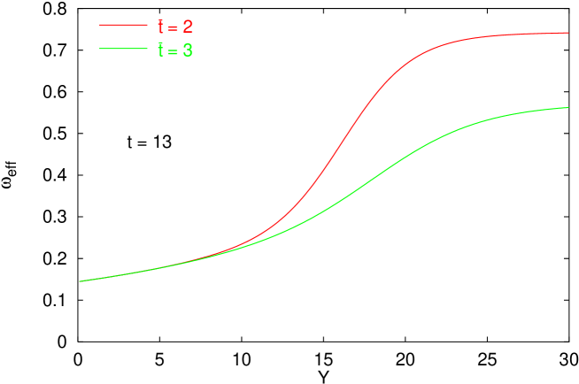
Figure 5.7: The effective intercept $\omega_{\text{eff}}$ as a function of $Y$ for $t=13$ and two different values of the infra-red cutoff $\bar{t}$.

Fig. 5.7 illustrates the basic behaviour of $\omega_{\text{eff}}$ for rather extreme kinematics — not intended to be phenomenologically relevant, but rather to show clearly the relevant features. Two values of the infra-red cutoff are considered. What is seen is that the exponent at first increases slowly and smoothly, and then at a certain threshold $Y$ increases rapidly towards $\omega_{\mathbb{P}}$. The saturation of $\omega_{\mathbb{P}}$ occurs later in $Y$ for increased $\bar{t}$ (i.e., decreased $\omega_{\mathbb{P}}$) as expected from (5.60). Traditional smooth diffusion into the infra-red would have led to the opposite behaviour, namely the higher $\bar{t}$ case (lower $\omega_{\mathbb{P}}$) being saturated first.

In order to have a closer look to the underlying physical mechanism, we analyse the $Y$-dependence of the so called Bartels’ cigar consisting in the contour plot of the function

$${{\mathcal{G}}(Y-y;t,t^{\prime}){\mathcal{G}}(y;t^{\prime},t_{0})\over{\mathcal{G}}(Y;t,t_{0})}\;.$$ (5.64)

Once one has fixed $Y$, $t$ and $t_{0}$, the $y$-section of Eq. (5.64) as a function of $t^{\prime}$ describes the relative importance of the intermediate states of different transverse momentum $k^{\prime}={\rm e}^{t^{\prime}/2}$ in the evolution of ${\mathcal{G}}$ from 0 to $Y$.

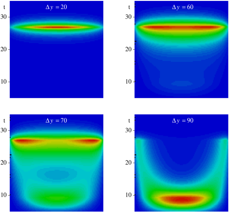
Figure 5.8: Domains of the dominant paths in transverse momentum $t^{\prime}$ and rapidity $y$ space for the evolution of the GGF in $Y$ between two hard and equal scales $t=t_{0}$. In the first plots the relevant paths stays in the perturbative region, their spread increasing with $Y$. The last plots show the sharp transition of the paths in the non perturbative region corresponding to the pomeron dominated cross section.

Let us start with a not too large rapidity interval $Y$ and consider for simplicity $t_{0}=t\gg 1$. The first plot of Fig. 5.8 shows that the domain of the dominant paths in transverse momentum-rapidity space, represented by the light coloured region, is restricted around the value of $t$ of the initial and final state, with a small spread. Increasing the value $Y$, the cigar gets thicker and thicker. In normal diffusion, the reach and the broadening of the cigar in the non perturbative region is gradual, according to its width $\sim\sqrt{\bar{\alpha}_{\mathrm{s}}(t)Y}$.

In the collinear model instead, we observe (Fig. 5.8) a jump (tunneling) in the IR region of an increasing fraction of paths as $Y$ gets larger, until all the relevant intermediate states belong to the strong coupling domain, thus providing the non perturbative regime mentioned in Sec. 5.7.

An impressing picture of the tunneling phenomenon can be obtained by plotting the distribution of transverse momenta in the middle of the evolution interval $Y/2$: Fig. 5.9 displays the contour plot of the function

$${|{\mathcal{G}}(Y/2;t,t^{\prime})|^{2}\over{\mathcal{G}}(Y;t,t)}$$ (5.65)

in $t^{\prime}$ and $Y/2$. In the left region (small evolution) the transverse momenta are spread around $t$ in the perturbative region and the small-$x$ effective growth exponent

$$\omega_{\text{eff}}(Y,t)\,\raisebox{0.37pt}{:}={{\rm d}\ln{\mathcal{G}}(Y;t,t)\over{\rm d}Y}$$ (5.66)

is given by the saddle point one $\omega_{s}(t)$ plus the ($Y$-derivative of the) corrections (5.61). For $Y>Y_{t}$ tunneling is at work and the small-$x$ exponent is given by $\omega_{\mathbb{P}}$.

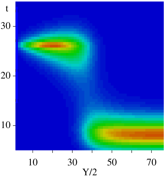
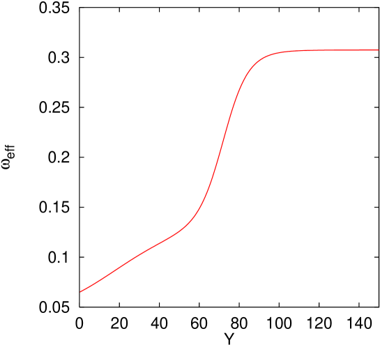
Figure 5.9: Middle section of the Bartels’ cigars of Fig. 5.8 for continuous value of $Y$ and the corresponding small-$x$ effective growth exponent

To conclude this chapter, we stress that all the estimates based on the collinear model are by no means intended to be quantitative results. This model reveals itself useful in order to justify some of the assumptions adopted in the treatment of the complete small-$x$ kernel such as the factorization properties and the $\omega$-expansion, and to clarify the role of the critical exponents $\omega_{s}(t)$, $\omega_{c}(t)$ and $\omega_{\mathbb{P}}$.

In particular, for two-scales processes, we have elucidated a completely new transition mechanism into the non perturbative domain which, for large enough energies $Y\gtrsim t(1+\omega_{\mathbb{P}})/(\omega_{\mathbb{P}}-\omega_{s}(t))$ and for sizeable values of $\omega_{\mathbb{P}}-\omega_{s}(t)$ may be spectacular.

Chapter 6 Conclusive remarks

This last and short chapter summarizes the basic results of the work presented in this thesis and indicates the main open questions and directions for future studies as well.

We have investigated the properties of QCD in the kinematic region of small-$x$ with particular attention to deeply inelastic scattering of electrons on hadrons and in particular to the physics at HERA. The most precise experimental results in the small-$x$ domain concerns the measurements of the $F_{2}$ structure function which clearly exhibits a marked rise (Fig. 2.1) towards low values of $x$ in a wide range of $Q^{2}$. Even though the standard DGLAP evolution equations are able to describe the whole set of data, nevertheless they have to be supplied with an initial condition (see Eq. (3.8)) for the partonic distribution functions which cannot be explained within the DGLAP approach itself. Furthermore, there is a variety of two-scale processes, e.g. $\gamma^{*}\gamma^{*}$ scattering and forward-jets, whose $x$-behaviour is determined independently of $Q^{2}$-evolution which is suppressed.

The natural framework where to study the small-$x$ behaviour of those inclusive processes is the BFKL one, where the large logarithmic coefficients of the perturbative series have been resummed at leading order and, recently, also at next-to-leading order. Even though the BFKL equation provides the right power-like shape for the small-$x$ growth of structure functions, nevertheless the quantitative estimate of the growth exponent is absolutely not compatible with its measurements (Fig. 3.1). This is true both at leading order — which overestimates the small-$x$ rise — and in the NL$x$ approximation, where the corrections are so large and negative that, for the accessible values of $Q^{2}$, the $x$-behaviour changes its slope (Fig. 3.13).

The analysis performed in Secs. 4.1 and 4.2 have shown that the responsibles of such large corrections and of the ensuing instability of the BFKL hierarchy are the big collinear contributions to the coefficient kernels in the BFKL expansion. More precisely, the coefficient kernels $K^{(n)}({\boldsymbol{k}},{\boldsymbol{k}}^{\prime})$ of Eq. (3.11) are affected by single and double logarithms of $k^{2}/k^{\prime}{}^{2}$ in the collinear limits $k^{2}\gg k^{\prime}{}^{2}$ and $k^{2}\ll k^{\prime}{}^{2}$. The single logarithms are essentially those predicted by the renormalization group equation which are responsibles for the logarithmic scaling violations in $Q^{2}$ for the partonic densities. The double logarithms, on the other hand, are due to the mismatch between the high energy factorization scale $s_{0}=kk_{0}$ — which is supposed to be the correct scale which allows the factorization formula (3.9) — and the Bjorken scale $s_{B}=\operatorname{{\rm Max}}(k^{2},k_{0}^{2})$ providing the relevant scaling variable $x_{B}\simeq s_{B}/s$ in the collinear limits $k^{2}\gg k_{0}^{2}$ and $k^{2}\ll k_{0}^{2}$.

Those large logarithms are unavoidable in the $\alpha_{\mathrm{s}}$-expansion of the BFKL kernel (3.11) and the corresponding series is oscillatory and unstable for not very small values of $\alpha_{\mathrm{s}}$. In addition, the total cross section stemming from the naïve NL$x$ truncation of that series may turn out to be negative in the very large $s$-limit! A resummation of the large collinear contributions mentioned before is therefore mandatory.

By a RG analysis of the collinear singularities of the GGF (4.20) and hence of the kernel (4.22,4.24) it is possible to determine the coefficients of single and double logarithms of the transverse momenta ${\boldsymbol{k}},{\boldsymbol{k}}_{0}$ to all orders in $\alpha_{\mathrm{s}}\ln 1/x$. The resummation of those logarithms can be accomplished by a suitable shift of the $\gamma$-singularities of the eigenvalue functions $\raisebox{1.5pt}{$\chi$}{}^{(n)}_{\omega}(\gamma)$ of the improved coefficient kernels of Eq. (4.19) as indicated in Eqs. (4.26). By then incorporating the constraints of the known L$x$ and NL$x$ BFKL eigenvalue functions, we are able to construct — up to NNL$x$ corrections — the resummed L$x$ and NL$x$ eigenvalues, given in Eqs. (4.36) and (4.46).

Having determined the collinear-resummed L$x$ and NL$x$ kernels, it remains the question of determining the improved GGF, i.e., the solution of Eq. (4.49). The technical difficulty in solving such an equation is mainly concerned with the running of $\alpha_{\mathrm{s}}(k^{2})$ and in particular with the singularity of its perturbative expression at the Landau point $k^{2}=\Lambda^{2}$. In practice, a suitable regularization of $\alpha_{\mathrm{s}}(k^{2})$ has to be adopted.

At this point we proceed in two directions: the first one consists in considering the large $t=\ln k^{2}/\Lambda^{2}$ regime ($t\gg t_{0}$) where perturbative (regularization independent) features and strong coupling (regularization dependent) ones are argued to factorize and therefore can be considered independently. The second one is to define a simplified small-$x$ model which can be exactly solved (at least numerically) where the qualitative features of the real case can be studied as well as the issue of factorization.

The complete small-$x$ equation has been studied in Chap. 4 where, in the regime $k^{2}\gg k_{0}^{2}$, the GGF is argued to assume the factorized form (4.57) in terms of a perturbative factor $F_{\omega}({\boldsymbol{k}})$ which obeys the homogeneous equation (4.58). The solution of the latter has been given in terms of the $\gamma$-representation (4.59) and of the $\omega$-expansion (4.66).

The merit of the $\omega$-expansion is to provide an effective eigenvalue function $\raisebox{1.5pt}{$\chi$}{}_{\omega}(\gamma)$ whose shape is stable even for sizeable values of the expansion parameter $\omega$ (Fig. 4.4) and whose error stemming from neglecting NNL$x$ contributions is much smaller than the corresponding NNL$x$ truncation of the BFKL kernel in the $\alpha_{\mathrm{s}}$-expansion. As far as the stability of the shape is concerned, this means that a minimum in the function $\gamma\mapsto\raisebox{1.5pt}{$\chi$}{}_{\omega}(\gamma)$ is always present, even for large values of $\omega$. Because of that, a stable saddle point exists, preventing us from negative cross sections and providing a small-$x$ growth exponent $\omega_{s}(t)$ — defined in Eq. (4.75) and plotted in Fig. 4.6 — which should be observable in some intermediate-$x$ regime (see Sec. 5.7). In the range $Q^{2}\simeq 4\div 40\text{ GeV}^{2}$, i.e., $\alpha_{\mathrm{s}}\simeq 0.2\div 0.3$, the critical exponent $\omega_{s}(t)\simeq 0.27\div 0.32$ is not far from the corresponding values of the HERA data.

It is to be noted that, while $\omega_{s}(t)$ decreases for large $t$, the trend of the experimental growth exponent is to increas with $Q^{2}$. This is due to the scaling violations, which the DGLAP approach takes into account by resumming the $\ln Q^{2}$ contributions which are not directly incorporated in $\omega_{s}(t)$. A more direct observation of the critical exponent $\omega_{s}(t)$ is expected from two-scale processes where the $Q^{2}$-evolution is less important (cfr. beginning of Chap. 3).

The error coming from the NL truncation in the $\omega$-expansion is uniformly (i.e., independently of $\gamma$) ${\mathcal{O}}(\omega^{2})$, the neglected coefficients having no $\gamma=0$ nor $\gamma=1$ singularities at all. This error is therefore of the same size as the ambiguity in the definition of $\raisebox{1.5pt}{$\chi$}{}_{1}^{\omega}$. The corresponding error in the saddle point condition (4.62) is a roughly $\gamma$-independent change of scale $\Delta(bt)={\mathcal{O}}(\omega)$, affecting the anomalous dimension with a relative uncertainty $\Delta\alpha_{\mathrm{s}}/\alpha_{\mathrm{s}}\sim\alpha_{\mathrm{s}}\omega$ while for the critical exponent $\Delta\omega_{s}(t)\sim\dot{\omega}_{s}(t)\Delta t$. The important thing to note is that all these errors are NNL$x$ and that their coefficients do not show a strong $t$-dependence.

In connection with the ambiguities of the finite order truncation, one can consider also the renormalization scale and scheme dependence as well as the resummation scheme dependence. In Sec. 4.10 it is shown that such dependences are very small and do not affect considerably the critical $\omega$-exponents $\omega_{s}$ and $\omega_{c}$.

The collinear model presented in Chap. 5 allows us to investigate in more detail the physical consequences of the collinear-resummed kernel. First of all, the model offers a method of analysis of non perturbative effects on the observable quantities, in particular on the very small-$x$ growth exponent (Sec. 5.4). The main results of that analysis is that, in two-scale processes, for large enough values of the external scales $k^{2}$ and $k_{0}^{2}$ and for not too large values of the energy $s$, there exists a regime governed by perturbative physics where the effective small-$x$ growth exponent is given by $\omega_{s}(t)$. A preliminary phenomenological analysis seems to indicate that the $x$-growth in $\gamma^{*}\gamma^{*}$ and forward-jet processes are similar, and consistent with the $\omega_{s}$ value quoted before. For increasing values of the energy, there is a transition point beyond which most of the exchanged gluons lie in the strong coupling region and the growth exponent is given by the “pomeron” which is of non perturbative nature. This transition mechanism does not take place continuously like “diffusion”. For this reason, we refer to it as “tunneling”.

The study of the RG improved small-$x$ equation has just begun and leaves many open questions yet, which hopefully will find an answer after further investigation. Just to mention some of them, there is to clarify the role of the critical exponent $\omega_{c}(t)$ — the true singularity of the resummed anomalous dimension. A second point concerns the evaluation of higher twist contributions stemming from poles in the effective eigenvalue functions at values of $\gamma<-\omega/2$ and $\gamma>1+\omega/2$. A preliminary study of such corrections can be done in the collinear model by suitably modifying the pole-structure of the eigenvalue. A major task concerns the implementation of unitarity which however should involve the study of strong coupling effects.

To conclude, small-$x$ physics emerges from our work as a rather unique framework where the perturbative and strong coupling features play a complementary role. I think we have shown that by combining $\ln 1/x$ and $\ln Q^{2}$ evolutions we can progress a great deal towards understanding the perturbative aspects of the problem. Further progress will require a deeper understanding of non perturbative physics.

Appendix A The Structure Functions in DIS

According to the definition of the kinematics variables of DIS in Sec. 1.4 (see Fig. 1.1),the transition matrix element is given, in the lowest order of the EM interaction, by

$$\langle l^{\prime}\,X|T|l\,H\rangle=\overline{u}_{\sigma^{\prime}}(p_{1}^{\prime})\,{\rm i}e\gamma^{\mu}\,u_{\sigma}(p_{1})\,{-{\rm i}\over q^{2}}\,\langle X|(-e)J_{\mu}(0)|p_{2},\lambda\rangle\;,$$ (A.1)

where $\sigma^{\prime}$, $\sigma$ and $\lambda$ are the spin components of the scattered electron, initial electron and target proton respectively, $e$ is the electronic EM charge and $J_{\mu}(x)$ is the quark part of the EM current.

The inclusive unpolarized differential cross section (with respect to the outgoing electron) is obtained by multiplying (A.1) by the appropriate phase space factor and reads

$$p_{1}^{\prime}{}^{0}\,{{\rm d}\sigma\over{\rm d}^{3}\vec{p}_{1}\!{}^{\prime}}={2\over s}\,{\alpha^{2}\over Q^{4}}\,L^{\mu\nu}W_{\mu\nu}\;,$$ (A.2)

where we have defined the leptonic tensor

$$L^{\mu\nu}(p_{1},q)\,\raisebox{0.37pt}{:}= {1\over 2}\sum_{\sigma,\sigma^{\prime}}\Big{(}\overline{u}_{\sigma^{\prime}}(p_{1}^{\prime})\gamma^{\mu}u_{\sigma}(p_{1})\Big{)}^{*}\Big{(}\overline{u}_{\sigma^{\prime}}(p_{1}^{\prime})\gamma^{\nu}u_{\sigma}(p_{1})\Big{)}$$ (A.3a)

$$= 2\left(p_{1}^{\mu}p_{1}^{\prime}{}^{\nu}+p_{1}^{\nu}p_{1}^{\prime}{}^{\mu}\right)+q^{2}g^{\mu\nu}$$ (A.3b)

and the hadronic tensor

$$W_{\mu\nu}(p_{2},q)\,\raisebox{0.37pt}{:}= {1\over 4\pi}\sum_{X}(2\pi)^{4}\delta^{4}(p_{2}+q-p_{X})\,{1\over 2}\sum_{\lambda}\langle p_{2},\lambda|J_{\mu}(0)|X\rangle\langle X|J_{\nu}(0)|p_{2},\lambda\rangle$$ (A.4a)

$$= {1\over 4\pi}\int{\rm d}^{4}z\;{\rm e}^{{\rm i}qz}\,{1\over 2}\sum_{\lambda}\langle p_{2},\lambda|[J_{\mu}(z),J_{\nu}(0)]|p_{2},\lambda\rangle\;.$$ (A.4b)

Because of current conservation at the hadronic vertex, $\partial_{\mu}J^{\mu}(z)|X\rangle=0$ and hence $q^{\mu}W_{\mu\nu}=0=q^{\nu}W_{\mu\nu}$. The most general form of the hadronic tensor fulfilling the requirements of Lorentz covariance, space-inversion and time-reversal conservation and current conservation is ($p_{2}q\equiv p_{2}\cdot q$)

$$W^{\mu\nu}=F_{1}\,\left({q^{\mu}q^{\nu}\over q^{2}}-g^{\mu\nu}\right)+F_{2}\,{1\over p_{2}q}\left(p_{2}^{\mu}-{p_{2}q\over q^{2}}q^{\mu}\right)\left(p_{2}^{\nu}-{p_{2}q\over q^{2}}q^{\nu}\right)\;,$$ (A.5)

where the Lorentz invariant coefficient $F_{i}(x,Q^{2}):i=1,2$ are called structure functions of the proton. It is worthwile to stress that the structure functions depends only on the Lorentz invariants of the lower vertex (the blob) in Fig. 1.1, i.e., on $x$ and $Q^{2}$.

Keeping $p_{2}$ and $q$ fixed, let’s introduce the longitudinal polarization unit vector

$$\epsilon_{L}^{\mu}(q)\,\raisebox{0.37pt}{:}={Q\over p_{2}q}\left[1+{M^{2}Q^{2}\over(p_{2}q)^{2}}\right]^{-\mbox{\small$\frac{1}{2}$}}\left(p_{2}^{\mu}-{p_{2}q\over q^{2}}q^{\mu}\right)\;,\quad q\cdot\epsilon_{L}=0\;,\quad\epsilon_{L}\cdot\epsilon_{L}=1$$ (A.6)

and a couple of transverse unit vectors $\epsilon_{1}$ and $\epsilon_{2}$ such that

$$q\cdot\epsilon_{i}=0\;,\quad\epsilon_{L}\cdot\epsilon_{i}=0\;,\quad\epsilon_{i}\cdot\epsilon_{i}=-1\;,\quad\epsilon_{1}\cdot\epsilon_{2}=0\;,\quad(i=1,2)\;.$$

The sets of vectors $\{\epsilon_{1},\epsilon_{2}\}$ and $\{\epsilon_{L},\epsilon_{1},\epsilon_{2}\}$ form pseudo-orthonormal basis for the subspaces $<p_{2},q>^{\perp}$ and $<q>^{\perp}$ respectively. Defining the projectors

$$\Pi^{\mu\nu}_{L} \,\raisebox{0.37pt}{:}=\epsilon_{L}^{\mu}\epsilon_{L}^{\nu}$$ (A.7)

$$\Pi^{\mu\nu}_{T} \,\raisebox{0.37pt}{:}=-(\overset{*}{\epsilon}{}{}_{1}^{\mu}\epsilon_{1}^{\nu}+\overset{*}{\epsilon}{}{}_{2}^{\mu}\epsilon_{2}^{\nu})$$ (A.8)

$$\Pi^{\mu\nu}_{\perp} \,\raisebox{0.37pt}{:}=\Pi^{\mu\nu}_{L}+\Pi^{\mu\nu}_{T}=g^{\mu\nu}-{q^{\mu}q^{\nu}\over q^{2}}$$ (A.9)

in the longitudinal, transverse and orthogonal (to $q^{\mu}$) space respectively, we can decompose the hadronic tensor as

$$W^{\mu\nu} =-F_{1}\,\Pi_{\perp}^{\mu\nu}+F_{2}\,{p_{2}q\over Q^{2}}\left(1+{Q^{2}\over\nu^{2}}\right)\Pi_{L}^{\mu\nu}$$ (A.10a)

$$=-F_{1}\,\Pi_{T}^{\mu\nu}+{F_{L}\over 2x}\,\Pi_{L}^{\mu\nu}$$ (A.10b)

$$={1\over 2x}\left[F_{L}\,\Pi_{\perp}^{\mu\nu}-\left(1+{Q^{2}\over\nu^{2}}\right)F_{2}\,\Pi_{T}^{\mu\nu}\right]\;,$$ (A.10c)

where the longitudinal structure function is given by

$$F_{L}(x,Q^{2})\,\raisebox{0.37pt}{:}=\left(1+{Q^{2}\over\nu^{2}}\right)F_{2}-2xF_{1}\;.$$ (A.11)

If we consider virtual photon absorption by a proton, the ensuing cross section involves just the hadronic tensor (A.4) and the former assumes the form

$$\sigma(\gamma^{*}\,H)\propto\overset{*}{\epsilon}{}{}^{\mu}\epsilon^{\nu}\,W_{\mu\nu}\;,$$ (A.12)

$\epsilon^{\mu}$ being the polarization vector of the virtual photon. It is easy then to extract any of the structure functions simply by choosing the appropriate vector $\epsilon^{\mu}$. If we parametrize the generic polarization vector $\epsilon^{\mu}=\lambda\epsilon_{L}+\tau\epsilon_{T}$ where $\epsilon_{T}$ is a unitary transverse vector, then $\overset{*}{\epsilon}{}{}^{\mu}\epsilon^{\nu}\,W_{\mu\nu}$ gives

• $F_{1}$ for $|\lambda|=0$ and $|\tau|=1$;

• $F_{L}$ for $|\lambda|=1$ and $|\tau|=0$;

• $F_{2}$ for $|\lambda|=|\tau|=2x/(1+{Q^{2}\over\nu^{2}})$.

A.1 $\boldsymbol{M,m\to 0}$ limit

For high values of the energy $\sqrt{s}$ and of the momentum transfer $Q$ with respect to the typical hadronic masses, the latter can safely be neglected, together with the electronic mass which is even smaller. In this case $\nu^{-1}=0$ and for the relevant kinematical variables holds

$$Q^{2}=xys\;.$$ (A.13)

In terms of these variables and of the azimuthal angle $\phi$ in the CM frame, the phase space element in Eq. (A.2) becomes

$$p_{1}^{\prime}{}^{0}\,{{\rm d}\over{\rm d}^{3}\vec{p}_{1}\!{}^{\prime}}={2sx^{2}\over Q^{2}}{{\rm d}\over{\rm d}x\,{\rm d}Q^{2}\,{\rm d}\phi}$$

so that we can write the differential cross section with respect to $x$, $Q^{2}$ and $\phi$ at fixed $s$ as

$${{\rm d}\sigma\over{\rm d}x\,{\rm d}Q^{2}\,{\rm d}\phi} ={Q^{2}\over 2x^{2}s}(\ref{sdd})={\alpha^{2}\over x^{2}s^{2}Q^{2}}L^{\mu\nu}W_{\mu\nu}$$

$$={2\alpha^{2}\over xQ^{4}}\left\{xy^{2}F_{1}+(1-y)F_{2}\right\}$$ (A.14a)

$$={\alpha^{2}\over xQ^{4}}\left\{[1+(1-y)^{2}]F_{2}-y^{2}F_{L}\right\}$$ (A.14b)

where $\alpha\,\raisebox{0.37pt}{:}=e^{2}/4\pi$ is the EM fine structure constant. Note that in this massless case $F_{L}=F_{2}-2xF_{1}$.

Appendix B Dimensional regularization

The dimensional regularization technique consists in performing the loop and phase space (divergent) integrals of Feynman diagrams and squared matrix elements in a modified space-time of generic dimension $D\neq 4$, where such integrals exist. The ensuing expressions are then analytically continued for complex values of $D$.

For our purposes, the main modifications with respect to the $D=4$ case concern the phase space measure ${\rm d}\phi^{(n)}$ and the expression of the coupling $\alpha_{\mathrm{s}}$.

The generally adopted convention for momentum integration is to replace the volume element as

$${{\rm d}^{4}k\over(2\pi)^{4}}\quad\longrightarrow\quad{{\rm d}^{D}k\over(2\pi)^{D}}\;.$$ (B.1)

Introducing the (half) extra-dimension parameter $\varepsilon:D=\raisebox{0.37pt}{:}\hskip 3.0pt4+2\varepsilon$, the phase space measure (2.46)

$${\rm d}\phi^{(2+n)}={1\over(2s)^{2}}{1\over(4\pi)^{n}}\prod_{i=1}^{n}{{\rm d}z_{i}\over z_{i}}\prod_{j=1}^{n+1}{{\rm d}{\boldsymbol{k}}_{j}\over(2\pi)^{2}}\quad\longrightarrow\quad{1\over(2s)^{2}}{1\over(4\pi)^{n}}\prod_{i=1}^{n}{{\rm d}z_{i}\over z_{i}}\prod_{j=1}^{n+1}{{\rm d}{\boldsymbol{k}}_{j}\over(2\pi)^{2+2\varepsilon}}\;,$$ (B.2)

i.e., only the $(2\pi)^{2}$ denominator under ${\rm d}{\boldsymbol{k}}_{j}$ is modified.

In addition, in going from L$x$ to NL$x$ approximation, also the longitudinal measure is modified. In particular the two-body phase space reads

$${\rm d}\phi^{(2)}={1\over 4s^{2}}{{\rm d}{\boldsymbol{k}}\over(2\pi)^{2+2\varepsilon}}$$ (B.3)

and the three-body one is

$${\rm d}\phi^{(3)}={1\over 16\pi s^{2}}{{\rm d}z_{1}\over z_{1}(1-z_{1})}{{\rm d}{\boldsymbol{k}}_{1}{\rm d}{\boldsymbol{k}}_{2}\over(2\pi)^{4+4\varepsilon}}\;.$$ (B.4)

In $4+2\varepsilon$ dimensions the QCD coupling constant $g$ acquire a mass-dimension $[g]=-\varepsilon$, therefore a massive parameter $\mu$ has to be introduced, so to consider $g\mu^{\varepsilon}$ as the effective dimensionless coupling. The convention generally adopted in the papers reporting the calculations of the NL$x$ BFKL kernel is to use the $\overline{MS}$ renormalization scheme and to define the dimensionless colour strength as

$$\alpha_{\mathrm{s}}\,\raisebox{0.37pt}{:}={g^{2}\mu^{2\varepsilon}\Gamma(1-\varepsilon)\over(4\pi)^{1+\varepsilon}}\;,$$ (B.5)

which reduces to the customary expression in the $\varepsilon\to 0$ limit. Accordingly, we have adopted the following definition for the Born impact factor:

$$h_{\text{\sf a}}^{(0)}({\boldsymbol{k}})\,\raisebox{0.37pt}{:}={2^{1+\varepsilon}C_{\text{\sf a}}\alpha_{\mathrm{s}}\over\sqrt{N_{c}^{2}-1}\,\Gamma(1-\varepsilon)}\,{1\over\mu^{2\varepsilon}{\boldsymbol{k}}^{2}}\;.$$ (B.6)

As transverse measure we keep the natural one

$${\rm d}{\boldsymbol{k}}\,\raisebox{0.37pt}{:}={\rm d}^{2+2\varepsilon}{\boldsymbol{k}}\quad;\quad\delta({\boldsymbol{k}})\,\raisebox{0.37pt}{:}=\delta^{2+2\varepsilon}({\boldsymbol{k}})\;.$$ (B.7)

Appendix C Integral representations for functions in transverse momentum space

C.1 The leading BFKL eigenvalue function

Given a set $\Omega$ of complex functions defined on a vectorial space $V$, an operator ${\mathcal{K}}$ acting on $\Omega$ is said to be rotationally invariant if it commutes with all the rotation operators on $V$. If ${\mathcal{K}}({\boldsymbol{k}},{\boldsymbol{k}}^{\prime})$ is the kernel of the linear integral operator ${\mathcal{K}}$, then ${\mathcal{K}}$ is rotationally invariant if and only if

$${\mathcal{K}}(R{\boldsymbol{k}},R{\boldsymbol{k}}^{\prime})={\mathcal{K}}({\boldsymbol{k}},{\boldsymbol{k}}^{\prime})\quad,\quad{\boldsymbol{k}},{\boldsymbol{k}}^{\prime}\in V$$ (C.1)

where $R$ is the generic rotation operator in $V$.

Let $S_{\lambda}$ denote the scaling operator on $\Omega$ defined by

$$[S_{\lambda}f]({\boldsymbol{k}})\,\raisebox{0.37pt}{:}=f(\lambda{\boldsymbol{k}})\quad,\quad f\in\Omega\;.$$ (C.2)

An operator ${\mathcal{K}}$ is said to be scale invariant if it commutes with $S_{\lambda}$ for all $\lambda>0$. In a $d$-dimensional vector space $V$, the integral operator ${\mathcal{K}}$ is scale invariant if and only if

$${\mathcal{K}}(\lambda{\boldsymbol{k}},\lambda{\boldsymbol{k}}^{\prime})=\lambda^{-d}{\mathcal{K}}({\boldsymbol{k}},{\boldsymbol{k}}^{\prime})\;.$$ (C.3)

Under rather general conditions, if the operator ${\mathcal{K}}$ is rotationally invariant, then it admits a complete set of eigenfunction $\{f_{j}:j\in J\}$ of the form

$$f_{j}({\boldsymbol{k}})=\Psi_{j}({\boldsymbol{k}}^{2})Y_{j}(\phi)$$ (C.4)

where $\phi$ denotes the set of angular variables and $Y_{j}$ is a spherical harmonic in $d$ dimensions. Furthermore, if ${\mathcal{K}}$ is also scale-invariant, the radial eigenfunctions $\Psi$ can only be powers of the variable ${\boldsymbol{k}}^{2}$.

The BFKL operator ${\mathcal{K}}$ acts on functions defined in the $d=2$ dimensional transverse space $V$; the only angular variable is the azimuthal angle $\phi$. The action of ${\mathcal{K}}$ on a generic function $f\in\Omega$ can be explicitly written as

$$[{\mathcal{K}}f]({\boldsymbol{k}})=\bar{\alpha}_{\mathrm{s}}\int{\rm d}{\boldsymbol{k}}^{\prime}{1\over\pi({\boldsymbol{k}}-{\boldsymbol{k}}^{\prime})^{2}}\left[f({\boldsymbol{k}}^{\prime})-{{\boldsymbol{k}}^{2}f({\boldsymbol{k}})\over 2{\boldsymbol{k}}^{\prime}{}^{2}}\right]$$ (C.5)

the first and second term corresponding to the real and virtual part of the kernel respectively. It is easy to check that, for fixed coupling $\bar{\alpha}_{\mathrm{s}}$, the BFKL kernel defines a rotationally and scale invariant operator.

Since in two dimensions spherical harmonics corresponds to complex exponentials

$$Y_{m}(\phi)={{\rm e}^{{\rm i}m\phi}\over\sqrt{\pi}}$$ (C.6)

the eigenfunctions of ${\mathcal{K}}$ are of the form

$$f_{\gamma,m}({\boldsymbol{k}})={\boldsymbol{k}}^{\gamma-1}{{\rm e}^{{\rm i}m\phi}\over\sqrt{\pi}}$$ (C.7)

and a complete set is obtained by allowing $m\in\mathbb{Z}$ and $\gamma=1/2+{\rm i}\nu:\nu\in\mathbb{R}$. The eigenfunctions (C.7) are normalized according to

$$\delta^{2}({\boldsymbol{k}}-{\boldsymbol{k}}_{0})=\sum_{m\in\mathbb{Z}}\int_{{1\over 2}-{\rm i}\infty}^{{1\over 2}+{\rm i}\infty}{{\rm d}\gamma\over 2\pi{\rm i}}\;f_{\gamma,m}({\boldsymbol{k}})f^{*}_{\gamma,m}({\boldsymbol{k}}_{0})$$ (C.8)

and satisfy the orthonormality conditions

$$\int{\rm d}{\boldsymbol{k}}\;f^{*}_{\gamma,m}({\boldsymbol{k}})f_{\gamma^{\prime},m^{\prime}}({\boldsymbol{k}})=2\pi\delta_{mm^{\prime}}\,\delta(\nu-\nu^{\prime})\quad,\quad\gamma=\mbox{\small$\frac{1}{2}$}+{\rm i}\nu\quad,\quad\gamma^{\prime}=\mbox{\small$\frac{1}{2}$}+{\rm i}\nu^{\prime}\;.$$ (C.9)

The IR finiteness of the kernel can be checked directly on the eigenfunctions. For simplicity we restrict ourselves to the $m=0$ case. By using the dimensional regularization in $d=2+2\varepsilon$ and the formula

$$\int{{\rm d}^{2+2\varepsilon}{\boldsymbol{k}}\over\pi^{1+\varepsilon}}\;{1\over[{\boldsymbol{k}}^{2}]^{1-\alpha}[({\boldsymbol{q}}-{\boldsymbol{k}})^{2}]^{1-\beta}}={\Gamma(1-\alpha-\beta-\varepsilon)\Gamma(\alpha+\varepsilon)\Gamma(\beta+\varepsilon)\over\Gamma(\alpha+\beta+2\varepsilon)\Gamma(1-\alpha)\Gamma(1-\beta)}({\boldsymbol{q}}^{2})^{\alpha+\beta+\varepsilon-1}$$ (C.10)

we get:

$$\int{{\rm d}^{2+2\varepsilon}{\boldsymbol{k}}^{\prime}\over\pi^{\varepsilon}}\;{\mathcal{K}}^{(\text{R})}({\boldsymbol{k}},{\boldsymbol{k}}^{\prime})({\boldsymbol{k}}^{\prime}{}^{2})^{\gamma-1} =\left[{1\over\varepsilon}+\psi(1)-\psi(\gamma)-\psi(1-\gamma)+{\mathcal{O}}(\varepsilon)\right]\bar{\alpha}_{\mathrm{s}}({\boldsymbol{k}}^{2})^{\varepsilon+\gamma-1}$$ (C.11)

$$\int{{\rm d}^{2+2\varepsilon}{\boldsymbol{k}}^{\prime}\over\pi^{\varepsilon}}\;{\mathcal{K}}^{(\text{V})}({\boldsymbol{k}},{\boldsymbol{k}}^{\prime})({\boldsymbol{k}}^{\prime}{}^{2})^{\gamma-1} =\left[-{1\over\varepsilon}+\psi(1)+{\mathcal{O}}(\varepsilon)\right]\bar{\alpha}_{\mathrm{s}}({\boldsymbol{k}}^{2})^{\varepsilon+\gamma-1}$$ (C.12)

where the real and virtual BFKL kernel are defined in Eqs. (2.54) and $\psi\,\raisebox{0.37pt}{:}=\Gamma^{\prime}/\Gamma$ is the logarithmic derivative of the gamma function. It is evident the singular behaviour of both the real and virtual terms in $d=2$ dimension corresponding to the poles in $\varepsilon$. However, when adding the two contributions, the poles cancel and in the $\varepsilon\to 0$ limit we recover the $m=0$ eigenvalue function $\chi(\gamma)\,\raisebox{0.37pt}{:}=\chi(\gamma,0)=2\psi(1)-\psi(\gamma)-\psi(1-\gamma)$. When acting on the general eigenfunction the kernel yields

$$\int{\rm d}{\boldsymbol{k}}\;{\mathcal{K}}({\boldsymbol{k}},{\boldsymbol{k}}^{\prime})\,f_{\gamma,m}({\boldsymbol{k}}^{\prime})=\bar{\alpha}_{\mathrm{s}}\chi(\gamma,m)\,f_{\gamma,m}({\boldsymbol{k}})$$ (C.13)

$$\chi(\gamma,m)=2\psi(1)-\psi\big{(}\gamma+{|m|\over 2}\big{)}-\psi\big{(}1-\gamma+{|m|\over 2}\big{)}\;.$$ (C.14)

C.2 Mellin representation in transverse momentum space

The BFKL kernel can be expressed in terms of its eigenfunctions (C.7) and its eigenvalues (C.13) by means of the spectral representation

$${\mathcal{K}}({\boldsymbol{k}},{\boldsymbol{k}}^{\prime})=\sum_{m\in\mathbb{Z}}\int_{{1\over 2}-{\rm i}\infty}^{{1\over 2}+{\rm i}\infty}{{\rm d}\gamma\over 2\pi{\rm i}}\;f_{\gamma,m}({\boldsymbol{k}})\bar{\alpha}_{\mathrm{s}}\chi(\gamma,m)f^{*}_{\gamma,m}({\boldsymbol{k}})\;$$ (C.15)

In particular, the azimuthal average of the kernel, defined by

$${\mathcal{K}}({\boldsymbol{k}}^{2},{\boldsymbol{k}}^{\prime}{}^{2})\,\raisebox{0.37pt}{:}=\int{{\rm d}\theta\over 2\pi}\;{\mathcal{K}}({\boldsymbol{k}},{\boldsymbol{k}}^{\prime})\quad,\quad\theta=\widehat{{\boldsymbol{k}}{\boldsymbol{k}}^{\prime}}$$ (C.16)

has $({\boldsymbol{k}}^{2})^{\gamma-1}$ as eigenfunctions and $\chi(\gamma)\,\raisebox{0.37pt}{:}=\chi(\gamma,0)$ as eigenvalue function. Thanks to Eq. (C.15), it can be given the integral representation

$${\mathcal{K}}({\boldsymbol{k}}^{2},{\boldsymbol{k}}^{\prime}{}^{2}) ={1\over\pi{\boldsymbol{k}}^{2}}\int_{{1\over 2}-{\rm i}\infty}^{{1\over 2}+{\rm i}\infty}{{\rm d}\gamma\over 2\pi{\rm i}}\;\left({{\boldsymbol{k}}^{2}\over{\boldsymbol{k}}^{\prime}{}^{2}}\right)^{\gamma}\bar{\alpha}_{\mathrm{s}}\chi(\gamma)\;,$$ (C.17)

$$\bar{\alpha}_{\mathrm{s}}\chi(\gamma) =\int{\rm d}{\boldsymbol{k}}\;\left({{\boldsymbol{k}}^{2}\over{\boldsymbol{k}}^{\prime}{}^{2}}\right)^{-\gamma}{\mathcal{K}}({\boldsymbol{k}}^{2},{\boldsymbol{k}}^{\prime}{}^{2})\;,$$ (C.18)

showing that $\chi(\gamma)$ is nothing but the Mellin transform of the azimuthally averaged kernel ${\mathcal{K}}$. This is due to the fact that the radial eigenfunctions of ${\mathcal{K}}$ are powers of ${\boldsymbol{k}}^{2}$.

The Mellin transformation allows to diagonalize convolutions of function in both longitudinal and transverse space, such as the high energy factorization formula (2.20). By defining

$$F_{2,\omega}(\gamma) \,\raisebox{0.37pt}{:}=\int_{0}^{\infty}{{\rm d}Q^{2}\over Q^{2}}\;\left({Q^{2}\over\Lambda^{2}}\right)^{-\gamma}\int_{0}^{1}{{\rm d}x\over x}\;x^{\omega}\,F_{2}(x,Q^{2})$$ (C.19a)

$$\hat{\sigma}_{\omega}(\gamma) \,\raisebox{0.37pt}{:}=\int_{0}^{\infty}{{\rm d}\rho\over\rho}\;\rho^{-\gamma}\int_{0}^{1}{{\rm d}\xi\over\xi}\;\xi^{\omega}\,\hat{\sigma}(\xi,\rho)\quad,\quad\xi={x\over z}\quad,\quad\rho={Q^{2}\over\Lambda^{2}}$$ (C.19b)

$${\mathcal{F}}_{\omega}(\gamma) \,\raisebox{0.37pt}{:}=\int{\rm d}{\boldsymbol{k}}\;\left({{\boldsymbol{k}}^{2}\over\Lambda^{2}}\right)^{-\gamma}\int_{0}^{1}{{\rm d}z\over z}\;z^{\omega}\,{\mathcal{F}}(z,{\boldsymbol{k}})$$ (C.19c)

the mentioned factorization formula can be written in the simple algebraic form (2.22) or as a ${\boldsymbol{k}}$-integral if the Mellin transform is carried out only in the longitudinal variables $x$ and $z$.

The Mellin transforms (C.19) can be inverted by using

$$F_{2}(x,Q^{2}) =\int_{{1\over 2}-{\rm i}\infty}^{{1\over 2}+{\rm i}\infty}{{\rm d}\gamma\over 2\pi{\rm i}}\;\left({Q^{2}\over\Lambda^{2}}\right)^{\gamma}\int{{\rm d}\omega\over 2\pi{\rm i}}\;x^{-\omega}\,F_{2,\omega}(\gamma)$$ (C.20a)

$$\hat{\sigma}\big{(}{x\over z},{Q^{2}\over\Lambda^{2}}\big{)} =\int_{{1\over 2}-{\rm i}\infty}^{{1\over 2}+{\rm i}\infty}{{\rm d}\gamma\over 2\pi{\rm i}}\;\left({Q^{2}\over\Lambda^{2}}\right)^{\gamma}\int{{\rm d}\omega\over 2\pi{\rm i}}\;\left({x\over z}\right)^{-\omega}\,\hat{\sigma}_{\omega}(\gamma)$$ (C.20b)

$${\mathcal{F}}(z,{\boldsymbol{k}}) ={1\over\pi{\boldsymbol{k}}^{2}}\int_{{1\over 2}-{\rm i}\infty}^{{1\over 2}+{\rm i}\infty}{{\rm d}\gamma\over 2\pi{\rm i}}\;\left({{\boldsymbol{k}}^{2}\over\Lambda^{2}}\right)^{\gamma}\int{{\rm d}\omega\over 2\pi{\rm i}}\;z^{-\omega}\,F_{\omega}(\gamma)$$ (C.20c)

where the integration in the complex $\omega$-plane is parallel to the imaginary axis and to the right of all the singularities of the integrating function.

Bibliography

- [1] W. Marciano and H. Pagels, Phys. Rep. 36C (1978) 138.
- [2] See, e.g., T. Muta in Foundations of QCD, World Scientific Lectures Notes in Physics-Vol. 5, 1987.
-
[3]
See, e.g.,
Yu.L. Dokshitzer, D.I. Dyakonov and S.I. Troyan, Phys. Rep. 58 (1980) 269 and also
G. Altarelli, Phys. Rep. 81 (1982) 1. - [4] See, e.g., L.V. Gribov, E.M. Levin and M.G. Ryskin, Phys. Rep. 100 (1983) 1.
- [5] A. Bassetto, M. Ciafaloni and G. Marchesini, Phys. Rep. 100 (1983) 201.
- [6] See, e.g., J.C. Collins, D.E. Soper and G. Sterman in Perturbative QCD, World Scientific, Singapore, 1989 and Refs. therein.
-
[7]
J.D. Bjorken, Phys. Rev. 179 (1969) 1547;
R.P. Feynman, Photon Hadron Interactions, W. A. Benjamin, New York, 1972. - [8] K.G. Wilson, Phys. Rev. 179 (1969) 1499.
- [9] N. Christ, B. Hasslacher and A.H. Mueller, Phys. Rev. D 6 (1972) 3543.
-
[10]
D.J. Gross and F. Wilczek, Phys. Rev. D 9 (1974) 980;
H. Georgi and H.D. Politzer, Phys. Rev. D 9 (1974) 416. -
[11]
V.N. Gribov and L.N. Lipatov, Sov. J. Nucl. Phys. 15 (1972) 438;
G. Altarelli and G. Parisi, Nucl. Phys. B 126 (1977) 298;
Yu.L. Dokshitzer, Sov. Phys. JETP 46 (1977) 641. -
[12]
S.Aid et al., H1 Collaboration, Nucl. Phys. B 470 (1996) 3;
The ZEUS Collaboration, Z. Physik C 69 (1996) 607. - [13] See, e.g., P.D.B. Collins and E.J. Squires in Regge Poles in Particle Physics – Springer Tracts in Modern Physics 45, Springer Verlag, Berlin, 1968.
- [14] A. Donnachie and P.V. Landshoff, Phys. Lett. B 296 (1992) 227.
-
[15]
S. Catani, M. Ciafaloni and F. Hautman, Phys. Lett. B 242 (1990) 97;
S. Catani, M. Ciafaloni and F.Hautman, Nucl. Phys. B 366 (1991) 135. -
[16]
L.N. Lipatov, Sov. J. Nucl. Phys. 23 (1976) 338;
E.A. Kuraev, L.N. Lipatov and V.S. Fadin, Sov. Phys. JETP 44 (1976) 443;
E.A. Kuraev, L.N. Lipatov and V.S. Fadin, Sov. Phys. JETP 45 (1977) 199;
Ya. Balitskii and L.N. Lipatov, Sov. J. Nucl. Phys. 28 (1978) 822. - [17] L.N. Lipatov in Perturbative QCD, World Scientific, Singapore, 1989.
- [18] M. Glück, E. Reya and A. Vogt, Z. Physik C 67 (1995) 433.
- [19] A.D. Martin, R.G. Roberts and W.J. Stirling, Phys. Lett. B 354 (1995) 155.
- [20] S.J. Brodsky, F. Hautmann and D. Soper, Phys. Rev. D 56 (1997) 6957.
- [21] See, e.g., P. Achard for L3 Collaboration, [hep-ex/9907016].
- [22] See, e.g., J. Kwiecinski, A.D. Martin and J.J. Outhawaite, Eur. Phys. J. C 9 (1999) 611 and Refs. therein.
- [23] See, e.g., J. Bartels and C. Ewerz, [hep-ph/9908454] and Refs. therein, in particular from [25] to [53].
- [24] V.S. Fadin and L.N. Lipatov, Phys. Lett. B 429 (1998) 127.
- [25] M. Ciafaloni and G. Camici, Phys. Lett. B 430 (1998) 349.
- [26] M. Ciafaloni, Phys. Lett. B 429 (1998) 363.
- [27] M. Ciafaloni and D. Colferai, Nucl. Phys. B 538 (1999) 187.
- [28] A.H. Mueller and H. Navelet, Nucl. Phys. B 282 (1987) 727.
-
[29]
V.S. Fadin and R. Fiore, Phys. Lett. B 294 (1992) 286;
V.S. Fadin and L.N. Lipatov, Nucl. Phys. B 406 (1993) 259;
V.S. Fadin, R. Fiore and A. Quartarolo, Phys. Rev. D 50 (1994) 2265. -
[30]
M. Ciafaloni, Nucl. Phys. B 296 (1988) 49;
S. Catani, F. Fiorani and G. Marchesini, Phys. Lett. B 234 (1990) 339; Nucl. Phys. B 336 (990) 18 - [31] L.N. Lipatov and V.S. Fadin, Sov. J. Nucl. Phys. 50 (1989) 712.
-
[32]
V. Del Duca, Phys. Rev. D 54 (1996) 989;Phys. Rev. D 54 (1996) 4474;
V. Del Duca and C.R. Schmidt, Phys. Rev. D 57 (1998) 4069. - [33] See, e.g., G. Camici and M. Ciafaloni, Nucl. Phys. B 467 (1996) 25 and Refs. therein.
- [34] W. Furmanski and R. Petronzio, Phys. Lett. B 97 (1980) 437.
- [35] I.A. Korchemskaya and G.P. Korchemsky, Phys. Lett. B 387 (1996) 346.
- [36] See, e.g., R. Brower and J. Weis, Rev. Mod. Phys. 47 (1975) 605.
- [37] See, e.g., M. Ciafaloni, C. De Tar and M.N. Misheloff, Phys. Rev. 188 (1969) 2522 and Refs. therein.
- [38] V.S. Fadin, R. Fiore and M.I. Kotsky, Phys. Lett. B 359 (1995) 181; Phys. Lett. B 387 (1996) 593.
- [39] G. Camici and M. Ciafaloni, Phys. Lett. B 412 (1997) 396.
-
[40]
V.S. Fadin, R. Fiore and A. Quartarolo, Phys. Rev. D 50 (1994) 5893;
V.S. Fadin, R. Fiore, and M. I. Kotsky, Phys. Lett. B 389 (1996) 737. -
[41]
G. Camici and M. Ciafaloni, Nucl. Phys. B 496 (1997) 305;
V.S. Fadin, R. Fiore, A. Flachi, and M.I. Kotsky, Phys. Lett. B 422 (1998) 287. -
[42]
V.S. Fadin and L.N. Lipatov, Nucl. Phys. B 477 (1996) 767;
V.S. Fadin, M.I. Kotsky and L.N. Lipatov, [hep-ph/9704267];Phys. Lett. B 415 (1997) 97; - [43] G. Camici and M. Ciafaloni, Phys. Lett. B 395 (1997) 118.
- [44] G. Camici and M. Ciafaloni, Nucl. Phys. B 496 (1997) 305.
- [45] J.C. Collins and J. Kwiecinski, Nucl. Phys. B 316 (1989) 307.
- [46] M. Ciafaloni, D. Colferai and G.P. Salam, [hep-ph/9907409], to be published in JHEP 9910 (1999) 017.
- [47] D.A. Ross, Phys. Lett. B 431 (1998) 161.
- [48] E.M. Levin, [hep-ph/9806228].
-
[49]
See, e.g., A.H. Mueller, Nucl. Phys. B 425 (1994) 471;
L.N. Lipatov, Nucl. Phys. B 452 (1995) 369;
J. Bartels, L.N. Lipatov and M. Wüsthoff, Nucl. Phys. B 464 (1996) 289. - [50] G.P. Salam, JHEP 9807 (1998) 19.
- [51] B. Andersson, G. Gustafson and J. Samuelsson, Nucl. Phys. B 467 (1996) 443.
- [52] M. Ciafaloni and D. Colferai, Phys. Lett. B 452 (1999) 372.
- [53] M. Ciafaloni, D. Colferai and G.P. Salam, [hep-ph/9905566] to be published in Phys. Rev. D 60 (1999) 114036.
- [54] M. Toller, Nuovo Cim. 37 n.2 (1965) 631.
- [55] S.J. Brodsky, V.S. Fadin, V.T. Kim, L.N. Lipatov and G.B. Pivovarov, JETP Lett. 70 (1999) 155.
- [56] S.J. Brodsky, G.P. Lepage and P.N. Mackenzie, Phys. Rev. 28 (1983) 228.
- [57] J. Bartels and H. Lotter, Phys. Lett. B 309 (1993) 400.
- [58] See, e.g., J.R. Forshaw and D.A. Ross, Quantum Chromodynamics and the Pomeron, Cambridge University Press, 1997.
- [59] Yu.V. Kovchegov and A.H. Mueller, Phys. Lett. B 439 (1998) 428.