hep-ph/0008291 DESY 00-121 Saclay/SPhT–T00/120

Next-to-leading order QCD corrections to parity-violating 3-jet observables for massive quarks in $\bf e^{+}e^{-}$ annihilation

W. Bernreuther^a,, A. Brandenburg^b, and P. Uwer^c,

Abstract:

In this work we provide all the missing ingredients for calculating parity-violating 3-jet observables in $e^{+}e^{-}$ collisions at next-to-leading order (NLO) including the full quark mass dependence. In particular we give explicit results for the one-loop corrections and for the singular contributions from real emission processes. Our formulae allow for the computation of the NLO 3-jet contributions to the forward-backward asymmetry for heavy flavours, which is – and will be – an important observable for electroweak physics at present and future $e^{+}e^{-}$ colliders.

I Introduction

The measurement of the forward-backward asymmetry $A_{\mbox{\scriptsize FB}}^{b}$ for $b$-quark production in $e^{+}e^{-}$ collisions at the Z peak provides one of the most precise determinations of the weak mixing angle ${\rm sin}^{2}\theta_{\rm eff}$. It can be determined with an error at the per mille level if the computations of $A_{\mbox{\scriptsize FB}}^{b}$ are at least as accurate as the present experimental precision of about two percent [1]. This implies, in particular, that perturbative and non-perturbative QCD corrections to the lowest order formula for $A_{\mbox{\scriptsize FB}}^{b}$ must be controlled to this level of accuracy.

As far as perturbative QCD corrections to this observable are concerned, the present knowledge is as follows. The order $\alpha_{s}$ contributions had been computed first for massless and then for massive quarks in ref. [2] and ref. [3, 4], respectively. These calculations, which used the quark direction for defining the asymmetry were later modified [5, 6, 7] to encompass the asymmetry with respect to the thrust axis, which is more relevant experimentally. The coefficient of the order $\alpha_{s}^{2}$ correction was computed first in ref. [8], for massless quarks using the quark axis definition, by numerical phase space integration. This result was recently corrected by a completely analytical [9] and by a numerical calculation [10]. In the latter reference the second-order corrections were also determined for the thrust axis definition.

For future applications to measurements at proposed linear $e^{+}e^{-}$ colliders the attained theoretical precision so far will not suffice. The forward-backward asymmetry will be a key observable for determining the electroweak couplings of the top quark above threshold – a fundamental task at a linear collider as far as top quark physics is concerned. Needless to say all radiative corrections must be determined for non-vanishing top quark mass. Moreover, there may be the option to run such a collider at the Z peak, aiming to increase the precision attained at LEP1/SLC significantly. For instance one may be able to measure $A_{\mbox{\scriptsize FB}}$ for $b$ and $c$ quarks to an accuracy of order 0.1 $\%$. (For a recent discussion, see ref. [11].)

Here we are concerned with the second-order QCD corrections to $A_{\mbox{\scriptsize FB}}$ for massive quarks $Q$. It is convenient to obtain this asymmetry by computing the individual contributions of the parton jets [8]. This break-up may also be useful from an experimental point of view, as the various contributions can be separately measured [12, 13, 14]. To order $\alpha_{s}^{2}$ the asymmetry is determined by the 2-, 3-, and 4-jet final states involving $Q$. The 4-jet contribution to $A_{\mbox{\scriptsize FB}}$ involves the known parity-violating piece of the Born matrix elements for $e^{+}e^{-}\to 4$ partons involving at least one ${\bar{Q}}Q$ pair (see, e.g. ref. [15]). The phase-space integration of these matrix elements in order to get $(A_{\mbox{\scriptsize FB}})_{\mbox{\scriptsize 4-jet}}$ for a given jet-resolution algorithm can be done numerically in a rather straightforward fashion. The computation of $(A_{\mbox{\scriptsize FB}})_{\mbox{\scriptsize 3-jet}}$ is highly non-trivial. Within the phase space slicing method [16, 17, 18], which we will use here, it amounts to determining first the parity-violating piece in the fully differential cross section for the reaction $e^{+}e^{-}\to 3$ resolved partons to order $\alpha_{s}^{2}$. This will be done in this paper. (For the definition of ‘resolved partons’ see section IV.) In addition the contribution to $(A_{\mbox{\scriptsize FB}})_{\mbox{\scriptsize 3-jet}}$ from $e^{+}e^{-}\to 4$ resolved partons is needed. It can be obtained from the known leading order matrix elements by a numerical integration in 4 space-time dimensions which incorporates a jet defining algorithm. This will be discussed elesewhere. The computation of $(A_{\mbox{\scriptsize FB}})_{\mbox{\scriptsize 2-jet}}$ for heavy quarks is beyond the scope of this work and remains to be done in the future.

Our paper is organized as follows. In section II we review the kinematics of the reaction and leading-order results, and define the 3-jet forward-backward asymmetry. In section III we discuss the calculation of the virtual corrections. In particular, the ultraviolet divergences, the infrared divergences, and the renormalization procedure is discussed. In section IV the singular contributions from the real corrections are calculated and the cancellation of the infrared divergences is checked. In section V we summarize our results and end with some conclusions.

II Kinematics and leading-order results

The leading order differential cross section for

$$e^{+}(p_{+})e^{-}(p_{-})\to Q(k_{Q})\bar{Q}(k_{\bar{Q}})g(k_{g})$$ (II.1)

can be written in the following form:

$$\frac{d\sigma}{d\phi d\!\cos\vartheta dxd\bar{x}} = \frac{3}{4}\frac{1}{(4\pi)^{3}}\sigma_{pt}\Bigg{\{}(1+\cos^{2}\vartheta)\,F_{1}+(1-3\cos^{2}\vartheta)\,F_{2}+\cos\vartheta\,F_{3}$$ (II.2)

$$+ \sin 2\vartheta\cos\phi\,F_{4}+\sin^{2}\vartheta\cos 2\phi\,F_{5}+\sin\vartheta\cos\phi\,F_{6}\Bigg{\}},$$

with

$$\sigma_{pt}=\sigma(e^{+}e^{-}\rightarrow\gamma^{\ast}\rightarrow\mu^{+}\mu^{-})=\frac{4\pi\alpha^{2}}{3s}.$$ (II.3)

In eq. (II.2), $\vartheta$ denotes the angle between the direction ${\bf p}_{-}$ of the incoming electron $e^{-}$ and the direction ${\bf k}_{Q}$ of the heavy quark $Q$. The angle $\phi$ is the oriented angle between the plane defined by $e^{-}$ and $Q$ and the plane defined by the quark anti-quark pair. The functions $F_{i}$ depend only on the scaled c.m. energies $x=2k\cdot k_{Q}/s$ and $\bar{x}=2k\cdot k_{\bar{Q}}/s$, and on the scaled mass square $z=m^{2}/s$ of the heavy quark and anti-quark, where $k=p_{+}+p_{-}$ and $s=k^{2}$. Note that the leading order differential cross section for a final state with $n\geq 4$ partons can be written in an analogous way in terms of the two angles $\vartheta$, $\phi$ and $3n-7$ variables that involve only the final state momenta. In higher orders absorptive parts give rise to three additional functions $F_{7,8,9}$ (cf. ref. [19]). The four functions $F_{1,2,4,5}$ are parity even. In particular, the 3-jet production rate is determined by $F_{1}$. In the case of massive quarks next-to-leading order results for $F_{1}$ were given in references [20, 21, 22, 23, 24, 25, 26, 27]. The two functions $F_{3}$ and $F_{6}$ are induced by the interference of a vector and an axial-vector current. In particular, using the quark-axis, the 3-jet forward-backward asymmetry is related to $F_{3}$ in leading order in the following way:

$$(A_{\mbox{\scriptsize FB}})_{\mbox{\scriptsize 3-jet}} = {\int_{0}^{1}d\cos\vartheta\int_{-\pi}^{\pi}d\phi\int_{D(y_{\rm cut})}dxd\bar{x}\frac{d\sigma}{d\phi d\!\cos\vartheta dxd\bar{x}}-\int_{-1}^{0}d\cos\vartheta\int_{-\pi}^{\pi}d\phi\int_{D(y_{\rm cut})}dxd\bar{x}\frac{d\sigma}{d\phi d\!\cos\vartheta dxd\bar{x}}\over\int_{-1}^{1}d\cos\vartheta\int_{-\pi}^{\pi}d\phi\int_{D(y_{\rm cut})}dxd\bar{x}\frac{d\sigma}{d\phi d\!\cos\vartheta dxd\bar{x}}}$$ (II.4)

$$= \frac{3}{8}{\int_{D(y_{\rm cut})}dxd\bar{x}F_{3}(x,\bar{x})\over\int_{D(y_{\rm cut})}dxd\bar{x}F_{1}(x,\bar{x})},$$

where $D(y_{\rm cut})$ defines, for a given jet finding algorithm and jet resolution parameter $y_{\rm cut}$, a region in the $(x,\bar{x})$ plane. Analogously, the function $F_{6}$ induces an azimuthal asymmetry

$$A_{\phi} = {\int_{0}^{\pi/2}d\phi\int_{-1}^{1}d\cos\vartheta\int_{D(y_{\rm cut})}dxd\bar{x}\frac{d\sigma}{d\phi d\!\cos\vartheta dxd\bar{x}}-\int_{\pi/2}^{\pi}d\phi\int_{-1}^{1}d\cos\vartheta\int_{D(y_{\rm cut})}dxd\bar{x}\frac{d\sigma}{d\phi d\!\cos\vartheta dxd\bar{x}}\over\int_{0}^{\pi/2}d\phi\int_{-1}^{1}d\cos\vartheta\int_{D(y_{\rm cut})}dxd\bar{x}\frac{d\sigma}{d\phi d\!\cos\vartheta dxd\bar{x}}+\int_{\pi/2}^{\pi}d\phi\int_{-1}^{1}d\cos\vartheta\int_{D(y_{\rm cut})}dxd\bar{x}\frac{d\sigma}{d\phi d\!\cos\vartheta dxd\bar{x}}}$$ (II.5)

$$= \frac{3}{8}{\int_{D(y_{\rm cut})}dxd\bar{x}F_{6}(x,\bar{x})\over\int_{D(y_{\rm cut})}dxd\bar{x}F_{1}(x,\bar{x})}.$$

Note that final states with two partons do not contribute to $A_{\phi}$. The electroweak couplings appearing in $F_{3,6}$ can be factored out as follows:

$$F_{3,6}=-g_{a}^{Q}(1-\lambda_{+}\lambda_{-})\left[Q_{Q}{\rm Re}\chi(g_{a}^{e}-f(\lambda_{+},\lambda_{-})g_{v}^{e})+g_{v}^{Q}|\chi|^{2}(f(\lambda_{+},\lambda_{-})(g_{v}^{e2}+g_{a}^{e2})-2g_{v}^{e}g_{a}^{e})\right]\tilde{F}_{3,6}.$$ (II.6)

In eq. (II.6),

$$g_{v}^{f} = T_{3}^{f}-2Q_{f}\sin^{2}\theta_{W},$$

$$g_{a}^{f} = T_{3}^{f},$$

$$\chi = {1\over 4\sin^{2}\theta_{W}\cos^{2}\theta_{W}}{s\over s-m_{Z}^{2}+im_{Z}\Gamma_{Z}},$$

$$f(\lambda_{+},\lambda_{-}) = {\lambda_{-}-\lambda_{+}\over 1-\lambda_{-}\lambda_{+}},$$ (II.7)

where $T_{3}^{f}$ is the third component of the weak isospin of the fermion $f$, $\theta_{W}$ is the weak mixing angle, and $\lambda_{\mp}$ denotes the longitudinal polarization of the electron (positron). In next-to-leading order in $\alpha_{s}$, additional contributions to $F_{3,6}$ with electroweak couplings different from those in eq. (II.6) are induced which we will not consider here. They are either proportional to ${\rm Im}\chi$ and thus suppressed formally in the electroweak coupling or generated by the triangle fermion loop diagrams depicted in figure 1(l), 1(m). The contribution of the triangle fermion loop is gauge independent and UV and IR finite. It was calculated some time ago in ref. [28].

The functions $\tilde{F}_{3,6}(x,\bar{x})$ may be expressed in terms of functions $h_{6}$, $h_{7}$ which appear in the decomposition of the so-called hadronic tensor as performed for example in references [29, 30, 31].

$$\tilde{F}_{3} = {1\over 2}\left[\sqrt{x^{2}-4z}h_{6}(x,\bar{x})+\sqrt{\bar{x}^{2}-4z}\cos\vartheta_{Q\bar{Q}}h_{7}(x,\bar{x})\right],$$

$$\tilde{F}_{6} = -{1\over 2}\sqrt{\bar{x}^{2}-4z}\sin\vartheta_{Q\bar{Q}}h_{7}(x,\bar{x}),$$ (II.8)

where $\vartheta_{Q\bar{Q}}$ is the angle between $Q$ and $\bar{Q}$ in the c.m. frame and we have

$$\cos\vartheta_{Q\bar{Q}}={2(1-x-\bar{x}+2z)+x\bar{x}\over\sqrt{x^{2}-4z}\sqrt{\bar{x}^{2}-4z}}.$$ (II.9)

It would seem pointless to trade $F_{3,6}$ for $h_{6,7}$ if it were not for the relation (which follows from CP invariance):

$$h_{7}(x,\bar{x})=-h_{6}(\bar{x},x).$$ (II.10)

The objective of this paper is to provide explicit expressions for the virtual corrections and for the singular parts of the real corrections to the function $h_{6}$. These corrections make up the complete contribution from three resolved partons at NLO, $h_{6}^{\mbox{\scriptsize 3 res., NLO}}$, which is ultraviolet and infrared finite. We regulate both infrared und ultraviolet singularities by continuation to $d=4-2\epsilon$ space-time dimensions. In this context one may wonder whether the above kinematics relations, in particular eq. (II) have to be modified for $d\not=4$. This is however not necessary if we consistently keep the momenta of electron and positron as well as the polarization vector of the photon/Z-boson in $d=4$ dimensions throughout the calculation. Note that this prescription still corresponds to the usual dimensional regularisation. In addition this prescription is compatible with the ‘t Hooft-Veltman prescription for $\gamma_{5}$ as we discuss later.

We finish this section by giving the Born result for $h_{6}$ in $d=4-2\epsilon$ dimensions:

$$h_{6}^{\mbox{\scriptsize LO}}(x,\bar{x})=16\*\pi\*\alpha_{s}\*(N^{2}-1)\*B\*\bigg{(}2\*x-(x\*\bar{x}+\bar{x}^{2}+2-4\*\bar{x})\*\epsilon-4\*{{x_{g}}\over 1-x}\*z\bigg{)}$$ (II.11)

with

$$B={1\over(1-x)\*(1-\bar{x})},$$ (II.12)

and the scaled gluon energy

$$x_{g}={2k\cdot k_{g}\over s}=2-x-\bar{x}.$$ (II.13)

Note that the terms proportional to $\epsilon$ in eq. (II.11) depend on the prescription used to treat $\gamma_{5}$ in $d$ dimensions. To derive the above equation we have used the prescription $\gamma_{\mu}\gamma_{5}\rightarrow{i\over 3!}\varepsilon_{\mu\beta\gamma\delta}\,\gamma^{\beta}\gamma^{\gamma}\gamma^{\delta}$ [32, 33]. We will discuss this issue in more detail in the next section together with the ultraviolet (UV) renormalization.

III Virtual corrections

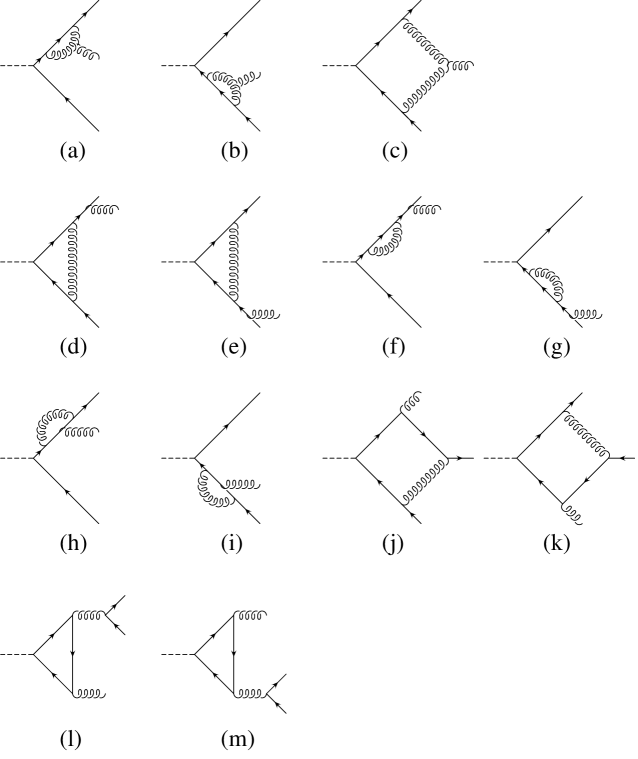
Figure 1: One-loop diagrams to $Z\to Q{\bar{Q}}g$.

In this section we will give analytic expressions for the virtual corrections to $h_{6}$, isolate the ultraviolet and infrared singularities, carry out the renormalization procedure, and discuss the treatment of $\gamma_{5}$.

We work in renormalized perturbation theory, which means that the bare quantities (fields and couplings) are expressed in terms of renormalized quantities. By this procedure one obtains two contributions: one is the original Lagrangian but now in terms of the renormalized quantities, the second contribution are the so-called counterterms:

$${\cal L}(\Psi_{0},A_{0},m_{0},g_{0})={\cal L}(\Psi_{R},A_{R},m_{R},g_{R})+{\cal L}_{ct}(\Psi_{R},A_{R},m_{R},g_{R}).$$ (III.1)

The first contribution yields the same Feynman rules as the bare Lagrangian but with the bare quantities replaced by renormalized ones. In the following we renormalize the quark field and the quark mass in the on-shell scheme, but treat the gluon field and the strong coupling in the modified minimal subtraction ($\overline{{\rm MS}}$) scheme [34, 35], taking into account the Lehmann–Symanzik–Zimmermann residue in the S-matrix element. Note that the conversion of the on-shell mass to the frequently used $\overline{{\rm MS}}$ mass can be performed at the end of the calculation. The quark mass in the on-shell scheme will be denoted in the following simply by $m$ for notational convenience.

While in the $\overline{{\rm MS}}$ scheme the renormalization constants contain only UV singularities, in the on-shell scheme they contain also infrared (IR) divergences. Although at the very end all the divergences cancel it is worthwhile to distinguish between UV and IR singularities so that one can check the UV renormalization and the IR finiteness independently.

To start with let us discuss the contribution of the one-loop diagrams before renormalization, that is the contribution from ${\cal L}(\Psi_{R},A_{R},m_{R},g_{R})$. Although tedious the calculation of the one-loop diagrams shown in figure 1 is in principle straightforward. We do not discuss here the contribution from diagrams l) and m) as mentioned earlier. Without going into the details we just review some techniques used in the calculation of the remaining diagrams. To calculate the one-loop corrections we decided to work in the background field gauge [36, 37] with the gauge parameter set to one. In this gauge the three-gluon vertex is simplified which leads to a reduction of the number of terms encountered in intermediate steps of the calculation. To reduce the one-loop tensor integrals to scalar one-loop integrals we used the Passarino-Veltman reduction procedure [38]. From the diagrams shown in figure 1 one can immediately read off the scalar box-integrals one encounters in the calculation. These integrals are

$$D_{0}^{d,l}=\frac{1}{i\pi^{2}}\int\!\!d^{d}l\frac{(2\pi\mu)^{(2\varepsilon)}}{(l^{2}+i\varepsilon)((l+k_{g})^{2}+i\varepsilon)((l+k_{Q}+k_{g})^{2}-m^{2}+i\varepsilon)((l-k_{\bar{Q}})^{2}-m^{2}+i\varepsilon)},$$ (III.2)

$$D_{0}^{d,sl,1}=\frac{1}{i\pi^{2}}\int\!\!d^{d}l\frac{(2\pi\mu)^{(2\varepsilon)}}{(l^{2}+i\varepsilon)((l+k_{Q})^{2}-m^{2}+i\varepsilon)((l+k_{Qg})^{2}-m^{2}+i\varepsilon)((l-k_{\bar{Q}})^{2}-m^{2}+i\varepsilon)},$$ (III.3)

$$D_{0}^{d,sl,2}=\left.D_{0}^{d,sl,1}\right|_{k_{Q}\leftrightarrow k_{\bar{Q}}},$$ (III.4)

with $k_{Qg}=k_{Q}+k_{g}$. Note that only the real parts of the one-loop integrals contribute to $h_{6}$ since we neglect terms in the electroweak couplings $\sim{\rm Im}\chi$. For simplicity we will leave out in the following the prescript Re in front of the integrals. All the lower-point integrals are defined with respect to the box-integrals. We adopted the notation from Passarino and Veltman [38] in which capital letters $A$, $B$,$\ldots$ are used to define one-point, two-point,$\ldots$ integrals. The kinematics is specified by denoting as argument the propagators which are kept with respect to the defining box-integrals. For example $C_{0}^{l}(1,2,3)$ which originates from $D_{0}^{l}$ is given by

$$C_{0}^{l}(1,2,3)=\frac{1}{i\pi^{2}}\int\!\!d^{d}l\frac{(2\pi\mu)^{(2\varepsilon)}}{(l^{2}+i\varepsilon)((l+k_{g})^{2}+i\varepsilon)((l+k_{Q}+k_{g})^{2}-m^{2}+i\varepsilon)}.$$ (III.5)

We have substituted the scalar box integrals in $d$ dimensions by box integrals in $d+2$ dimensions using the relation

$$D_{27}^{d}=-{1\over 2\pi}D_{0}^{d+2},$$ (III.6)

where $D_{27}^{d}$ is the coefficient of $g_{\mu\nu}$ in the decomposition of the four-point tensor integral $D^{d}_{\mu\nu}$ (cf. eq. (F.3) in ref. [38]), which in turn can be expressed as a linear combination of the scalar box integral $D_{0}^{d}$ and scalar triangle integrals $C_{0}$ in $d$ dimensions. Since the box integrals are finite in 6 dimensions, all IR singularities reside in triangle integrals after this substitution. As a gain, the coefficients of the triangle integrals become much simpler. This is clear, since the coefficient that multiplies the sum of all IR singular terms has to be proportional to the Born result.

We may group the diagrams shown in figure 1 according to their colour structure in terms of the colour matrices $T_{a}$ of the SU(N) gauge group. In particular, we distinguish between contributions which are dominant in the number of colours (‘leading-colour’) and contributions which are suppressed in the number of colours (‘subleading-colour’). The different colour structures are separately gauge independent. The diagrams a, b, c are proportional to $N(T_{a})_{c_{Q}c_{\bar{Q}}}$ where $a$ is the colour index of the gluon and $c_{Q}$ $(c_{\bar{Q}})$ the colour index of the (anti-) quark. The diagrams h, j, k, l are proportional to $1/N(T_{a})_{c_{Q}c_{\bar{Q}}}$. They are purely sub-leading in the number of colours. The diagrams d, e, f, g are proportional to $(N-1/N)(T_{a})_{c_{Q}c_{\bar{Q}}}$. These diagrams contribute to the leading as well as to the subleading parts.

To organize the next-to-leading order virtual corrections $h_{6}^{\mbox{\scriptsize virt., NLO}}$ for $h_{6}$ it is convenient to separate them into different contributions. First we split the result into a contribution from the loop diagrams (figure 1) and a contribution from the renormalization procedure $h_{6}^{\mbox{\scriptsize virt., ren.}}$. The contribution from the loop-diagrams is further decomposed into a UV divergent ($h_{6}^{\mbox{\scriptsize virt., UV div.}}$), a IR divergent ($h_{6}^{\mbox{\scriptsize virt., IR div.}}$) and a finite part ($h_{6}^{\mbox{\scriptsize virt., fin.}}$). We thus arrive at the following decomposition:

$$h_{6}^{\mbox{\scriptsize virt., NLO}}=h_{6}^{\mbox{\scriptsize virt., UV div.}}+h_{6}^{\mbox{\scriptsize virt., IR div.}}+h_{6}^{\mbox{\scriptsize virt., fin.}}+h_{6}^{\mbox{\scriptsize virt., ren.}}.$$ (III.7)

We define the singular contribution by taking only the pole-part of the loop-integrals but keeping the $\epsilon$-dependence in the prefactors.

III.1 UV singularities

All the UV singularities in a one-loop calculation appear in the scalar one- and two-point integrals. Defining the finite contributions $\overline{A}(m^{2})$, $\overline{B}_{0}(i,j)$ of these integrals by

$$A(m^{2}) = r_{\Gamma}\left({m^{2}\over 4\pi\mu^{2}}\right)^{-\epsilon}m^{2}{1\over\epsilon}+\overline{A}(m^{2}),$$

$$B_{0}(i,j) = r_{\Gamma}\left({m^{2}\over 4\pi\mu^{2}}\right)^{-\epsilon}{1\over\epsilon}+\overline{B}_{0}(i,j),$$ (III.8)

where $r_{\Gamma}$ is the usual one-loop factor:

$$r_{\Gamma}={\Gamma(1+\epsilon)\*\Gamma^{2}(1-\epsilon)\over\Gamma(1-2\epsilon)},$$ (III.9)

the contribution from the pole-part of these integrals is given by

$$h_{6}^{\mbox{\scriptsize virt., UV div.}} = {r_{\Gamma}{1\over\epsilon}\left({m^{2}\over 4\pi\mu^{2}}\right)^{-\epsilon}}\bigg{\{}{\alpha_{s}\over 2\*\pi}\*C_{F}\*h_{6}^{\mbox{\scriptsize LO}}+24\*\alpha_{s}^{2}\*(N^{2}-1)\*C_{F}\*\delta h_{6}$$ (III.10)

$$+ 8\*\alpha_{s}^{2}\*(N^{2}-1)\*C_{F}\*B\*\epsilon\*\bigg{(}1+x-2\*\bar{x}+(1-\bar{x})\*{\bar{x}\over x}$$

$$+ z\*\bigg{[}2\*B\*((\bar{x}^{2}-2\*x)\*(1-x)+(2-3\*x)\*(1-\bar{x}))+g_{1}\*{x^{2}-4\*z\over x\*(1-x)}+4\*z\*B\*(2\*{(1-\bar{x})^{2}\over 1-x}+{x_{g}})\bigg{]}\bigg{)}$$

$$+ 16\*\alpha_{s}^{2}\*C_{F}\*B\*\epsilon\*({1\over{x_{g}}}\*(x\*\bar{x}-4\*\bar{x}+2+\bar{x}^{2})-2\*z\*{x_{g}}\*B\*(x-\bar{x}))+O(\epsilon^{2})\bigg{\}}$$

with

$$\delta h_{6} = B^{2}\*\bigg{(}\bigg{[}-2\*{(x^{2}-3\*x-\bar{x}^{2}\*x+3\*x\*\bar{x}+2\*\bar{x}^{2}-4\*\bar{x}+2)}-{{x_{g}}\*(\bar{x}^{2}+x\*\bar{x}-4\*\bar{x}+2)}\*\epsilon\bigg{]}\*z$$ (III.11)

$$-4\*{1\over 1-x}\*(-5\*\bar{x}-3\*x+2\*\bar{x}^{2}+4+x^{2}+x\*\bar{x})\*z^{2}\bigg{)},$$

and

$$g_{1}=-{(1-x)\*(x-2\*\bar{x})\over(x^{2}-4\*z)^{2}}\*(x\*(\bar{x}+x)-2\*(1-{x_{g}})).$$ (III.12)

The finite contributions involving $\overline{A}$, $\overline{B}_{0}$ are given in section III.3. The cancellation of the UV singularities by the renormalization procedure will be discussed in sec. III.4.

III.2 Soft and collinear singularities

To start with let us consider the soft and collinear singularities appearing in the leading-colour contribution. As mentioned earlier we use the box-integral in $6-2\epsilon$ dimensions rather than in $4-2\epsilon$ dimensions. The one- and two-point integrals encountered in this calculation and the box integrals in $6-2\epsilon$ dimension do not contain IR singularities. As a consequence all IR singularities appear in the triangle integrals. Using the results for the integrals given in ref. [21] we see that only $C_{0}^{l}(1,2,3)$ and $C_{0}^{l}(1,2,4)$ are IR divergent. The contribution from the two integrals is given by

$$\left.h_{6}^{\mbox{\scriptsize virt., IR div.}}\right|_{\mbox{\scriptsize lead. colour}} = -{\alpha_{s}\over 2\*\pi}\*{N}\*h_{6}^{\mbox{\scriptsize LO}}\*\left\{(1-\bar{x})\,\*s\,\,\*C_{0}^{l}(1,2,3)+(1-x)\,\*s\,\,\*C_{0}^{l}(1,2,4)\right\}.$$ (III.13)

Using ref. [21]

$$(1-\bar{x})\,\*s\,\,\*C_{0}^{l}(1,2,3)$$ (III.14)

$$= r_{\Gamma}\*\left({4\*\pi\*\mu^{2}\over m^{2}}\right)^{\epsilon}\*\Bigg{\{}{1\over 2}\*{1\over\epsilon^{2}}-{1\over\epsilon}\*\ln({t_{Qg}\over m^{2}})+\ln({t_{Qg}\over m^{2}})^{2}-{7\over 12}\*\pi^{2}-\,{{\rm Li}_{2}}({{1\over\beta}})-{1\over 2}\*\ln(\beta)^{2}\Bigg{\}}+O(\epsilon)$$

$$\equiv r_{\Gamma}\*\left({4\*\pi\*\mu^{2}\over m^{2}}\right)^{\epsilon}\*\Bigg{\{}{1\over 2}\*{1\over\epsilon^{2}}-{1\over\epsilon}\*\ln({t_{Qg}\over m^{2}})\Bigg{\}}+(1-\bar{x})\,\*s\,\,\*\overline{C}_{0}^{l}(1,2,3)$$

with

$$\beta={1-\bar{x}+z\over z},\quad t_{ij}=2k_{i}\cdot k_{j},$$ (III.15)

and $C_{0}^{l}(1,2,3)\stackrel{{\scriptstyle x\leftrightarrow\bar{x}}}{{\longrightarrow}}C_{0}^{l}(1,2,4)$ we obtain for the singular part

$$\left.h_{6}^{\mbox{\scriptsize virt., IR div.}}\right|_{\mbox{\scriptsize lead. colour}} = -{\alpha_{s}\over 2\*\pi}\*r_{\Gamma}\*\left({4\*\pi\*\mu^{2}\over m^{2}}\right)^{\epsilon}\*{N}\*h_{6}^{\mbox{\scriptsize LO}}\*\left\{{1\over\epsilon^{2}}-{1\over\epsilon}\*\ln({t_{Qg}\over m^{2}})-{1\over\epsilon}\*\ln({t_{\bar{Q}g}\over m^{2}})\right\}.$$ (III.16)

In the sub-leading colour contribution only $C_{0}^{sl,1}(1,2,4)$ contains singularities. The contribution from $C_{0}^{sl,1}(1,2,4)$ is given by

$$\left.h_{6}^{\mbox{\scriptsize virt., IR div.}}\right|_{\mbox{\scriptsize subl. colour}}={\alpha_{s}\over 2\*\pi}\*{1\over N}\*h_{6}^{\mbox{\scriptsize LO}}\*(x+\bar{x}-2\*z-1)\,\*s\,\,\*C_{0}^{sl,1}(1,2,4).$$ (III.17)

Using ref. [21]

$$(x+\bar{x}-2\*z-1)\,\*s\,\,\*C_{0}^{sl,1}(1,2,4)$$

$$= r_{\Gamma}\*\left({4\*\pi\*\mu^{2}\over m^{2}}\right)^{\epsilon}\*{1+\omega^{2}\over 1-\omega^{2}}\*\Bigg{\{}{1\over\epsilon}\*\ln(\omega)+{1\over 2}\*\ln^{2}(\omega)+2\*\,\,{{\rm Li}_{2}}(1-\omega)-\pi^{2}\Bigg{\}}+O(\epsilon)$$

$$\equiv r_{\Gamma}\*\left({4\*\pi\*\mu^{2}\over m^{2}}\right)^{\epsilon}\*{1+\omega^{2}\over 1-\omega^{2}}{1\over\epsilon}\*\ln(\omega)+(x+\bar{x}-2\*z-1)\,\*s\,\,\*\overline{C}_{0}^{sl,1}(1,2,4)$$

with

$$\omega={1-\sqrt{1-{4\*z\over x+\bar{x}-1}}\over 1+\sqrt{1-{4\*z\over x+\bar{x}-1}}}$$ (III.19)

we obtain

$$\left.h_{6}^{\mbox{\scriptsize virt., IR div.}}\right|_{\mbox{\scriptsize subl. colour}}={\alpha_{s}\over 2\*\pi}\*{1\over N}\*h_{6}^{\mbox{\scriptsize LO}}\*r_{\Gamma}\*\left({4\*\pi\*\mu^{2}\over m^{2}}\right)^{\epsilon}{1\over\epsilon}\*{1+\omega^{2}\over 1-\omega^{2}}\*\ln(\omega)$$ (III.20)

for the singular part. There are additional IR singular contributions from the counterterm diagrams. They will be discussed in section III.4. Furthermore we note that $h_{6}^{\mbox{\scriptsize LO}}$ in the equations above is the result in $d$ dimensions. This follows immediately from the general properties of soft and collinear limits in QCD. This is the reason why no ‘$\gamma_{5}$-problem’ arises from the IR singularities: Given the fact that the IR singularities from the real corrections are also proportional to the Born result in $d$ dimensions, finite contributions which would be sensitive to the $\gamma_{5}$-prescription cancel together with the IR singularities, as long as one uses the same $\gamma_{5}$-prescription for the virtual and the real corrections.

III.3 Finite contributions

Given the divergent contributions shown in eq. (III.10), eq. (III.16) and eq. (III.20) we obtain the following result for the finite parts:

$$h_{6}^{\mbox{\scriptsize virt., fin.}}=\alpha_{s}^{2}\,C_{F}N^{2}\left.h_{6}^{\mbox{\scriptsize virt., fin.}}\right|_{\mbox{\scriptsize lead. colour}}+\,\,\alpha_{s}^{2}\,C_{F}\left.h_{6}^{\mbox{\scriptsize virt., fin.}}\right|_{\mbox{\scriptsize subl. colour}},$$ (III.21)

with

$${1\over 4\*B}\left.h_{6}^{\mbox{\scriptsize virt., fin.}}\right|_{\mbox{\scriptsize lead. colour}}=$$

$$-8\*\bigg{\{}-x\*(1-{x_{g}})+z\*B\*[x^{3}+5\*x^{2}\*\bar{x}-6\*x^{2}+10\*x+5\*x\*\bar{x}^{2}-16\*x\*\bar{x}+12\*\bar{x}-10\*\bar{x}^{2}-4+3\*\bar{x}^{3}]$$

$$-4\*B\*{x_{g}}\*z^{2}\*\bigg{[}{(1-\bar{x})^{2}\over 1-x}+{x_{g}}\bigg{]}\bigg{\}}\*s\*{1\over\pi}\*D_{0}^{d=6,l}$$

$$+\bigg{\{}2\*B\*\bigg{[}1+4\*\bar{x}\*(1-\bar{x})+x\*(\bar{x}-2)\*\bar{x}+2\*(1-\bar{x})^{2}\*\bar{x}\*{1\over x^{2}}-(1-\bar{x})\*(1+2\*\bar{x}\*(1-\bar{x}))\*{1\over x}\bigg{]}$$

$$+z\*\bigg{[}-8\*B\*(2\*{(1-\bar{x})^{2}\over 1-x}+{x_{g}})+{x^{2}\*\bar{x}+8\*\bar{x}-7\*x\*\bar{x}-6\*x^{2}+24\*x-22\over(1-x+z)\*(2-x)\*(1-x)}-{\bar{x}^{2}+\bar{x}-4\over(1-\bar{x}+z)\*(1-\bar{x})}$$

$$+8\*g_{1}\*{x^{2}-4\*z\over(2-x)\*(1-x)\*x^{2}}\bigg{]}\bigg{\}}\*{1\over s}\*\overline{A}(zs)$$

$$+\bigg{\{}6-10\*x-6\*(1-x)\*{1\over\bar{x}}+z\*\bigg{[}1-\bar{x}+4\*x+g_{2}\*(1-{2\over\bar{x}})-4\*{1+x-4\*z\over 1-\bar{x}}-{\bar{x}^{2}+\bar{x}-4\over 1-\bar{x}+z}\bigg{]}\bigg{\}}\*\overline{B}_{0}^{l}(1,3)$$

$$+\bigg{\{}16\*x-z\*\bigg{[}g_{2}+3\*g_{1}\*x+B\*\bigg{(}5\*x^{2}\*\bar{x}+11\*x^{2}-55\*x+52\*x\*\bar{x}-13\*x\*\bar{x}^{2}+64\*(1-\bar{x})-33\*\bar{x}\*(1-\bar{x})\bigg{)}$$

$$-\bigg{(}4\*x^{3}-x^{2}\*(2+3\*\bar{x})+x\*(4-\bar{x}-4\*\bar{x}^{2})+2-10\*\bar{x}+14\*\bar{x}^{2}-4\*{1-\bar{x}\over 1-x}\bigg{)}\*{1\over x^{2}-4\*z}\bigg{]}$$

$$-32\*B\*z^{2}\*\bigg{[}1-x+{(1-\bar{x})^{2}\over 1-x}\bigg{]}\bigg{\}}\*\overline{B}_{0}^{l}(2,3)$$

$$-\bigg{\{}-2\*\bar{x}^{2}\*{1\over x}-2\*\bar{x}\*(1-{x_{g}})\*{1\over x^{2}}+z\*\bigg{[}-3+3\*g_{1}\*(2-x)-x+4\*\bar{x}-{8\*\bar{x}\over 1-x}$$

$$+\bigg{(}10+2\*\bar{x}+10\*\bar{x}^{2}-x^{2}\*(4+3\*\bar{x})-x\*(2+\bar{x}+4\*\bar{x}^{2})+4\*x^{3}-8\*{1-\bar{x}\over 2-x}+4\*{1-\bar{x}\over 1-x}-8\*(1-{x_{g}})\*{\bar{x}\over x^{2}}-8\*{\bar{x}^{2}\over x}$$

$$\bigg{)}\*{1\over x^{2}-4\*z}-{(x^{2}\*\bar{x}+8\*\bar{x}-7\*x\*\bar{x}-6\*x^{2}+24\*x-22)\over(2-x)\*(1-x+z)}\bigg{]}+{16\*z^{2}\over 1-x}\bigg{\}}\*\overline{B}_{0}^{l}(2,4)$$

$$+2\*\bigg{\{}-x-3\*(1-{x_{g}})\*{1\over\bar{x}}+(1-\bar{x})\*\bar{x}\*{1\over x^{2}}-\bar{x}\*(1+\bar{x})\*{1\over x}+z\*\bigg{[}3\*g_{1}+g_{2}\*{1\over\bar{x}}+{8\*{x_{g}}\over 1-x}$$

$$+(2+6\*\bar{x}-2\*x^{2}-x\*(3-\bar{x})+4\*{1-\bar{x}\over 1-x}+4\*(1-\bar{x})\*\bar{x}\*{1\over x^{2}}-4\*\bar{x}\*(1+\bar{x})\*{1\over x})\*{1\over x^{2}-4\*z}\bigg{]}\bigg{\}}\*\overline{B}_{0}^{l}(3,4)$$

$$-8\*(1-\bar{x})\*\bigg{\{}x-{2\*{x_{g}}\*z\over 1-x}\bigg{\}}\*s\,\*\overline{C}_{0}^{l}(1,2,3)-8\*(1-x)\*\bigg{\{}x-{2\*{x_{g}}\*z\over 1-x}\bigg{\}}\*s\,\*\overline{C}_{0}^{l}(1,2,4)$$

$$+2\*z\*(1-\bar{x})\*\bigg{\{}{1\over 2}\*g_{2}+7+2\*x-{1\over 2}\*(1+\bar{x})\*\bigg{[}1+{8\over 1-x}\bigg{]}+8\*z\*\bigg{[}{1\over 1-\bar{x}}+{2\*{x_{g}}\over(1-x)^{2}}\bigg{]}\bigg{\}}\*s\,\*C_{0}^{l}(1,3,4)$$

$$-2\*z\*\bigg{\{}-{3\over 2}\*g_{1}\*(1-x)\*x-{3\over 2}+3\*x+{1\over 2}\*x^{2}+4\*{1-x^{2}\over 1-\bar{x}}-2\*x\*\bar{x}-8\*z\*\bigg{[}1+2\*{1-x\over 1-\bar{x}}\bigg{]}$$

$$-{1\over 2}\*\bigg{[}18\*x\*\bar{x}^{2}-14\*\bar{x}^{2}-4\*\bar{x}^{2}\*x^{2}+2\*x^{2}\*\bar{x}+6\*\bar{x}-9\*x\*\bar{x}-3\*x^{3}\*\bar{x}+4\*x^{4}$$

$$+2\*(1-x)\*(1+3\*x^{2})\bigg{]}\*{1\over x^{2}-4\*z}\bigg{\}}\*s\,\*C_{0}^{l}(2,3,4)$$

and

$${1\over 4\*B}\left.h_{6}^{\mbox{\scriptsize virt., fin.}}\right|_{\mbox{\scriptsize subl. colour}}=$$

$$-2\*\bigg{\{}2\*(1-\bar{x})+z\*\bigg{[}\bar{x}-2\*{1-2\*x\over 1-\bar{x}}-4\*{z\*{x_{g}}\over(1-\bar{x})^{2}}\bigg{]}\bigg{\}}\*\overline{B}_{0}^{l}(1,3)$$

$$+4\*z\*\bigg{\{}-B\*(2\*x^{2}+3\*x\*\bar{x}-5\*x-x\*\bar{x}^{2}+3-2\*\bar{x})+2\*z\*B^{2}\*(x-\bar{x})\*{x_{g}}^{2}-{(1-x)\*(x-2\*\bar{x})\over x^{2}-4\*z}$$

$$+{(\bar{x}-2)\*{x_{g}}\over 1-{x_{g}}-4\*z}\bigg{\}}\*\overline{B}_{0}^{l}(2,3)$$

$$+2\*\bigg{\{}2\*\bar{x}\*{1-x\over x}+z\*\bigg{[}4-\bar{x}+2\*{\bar{x}\over 1-x}-4\*{z\*{x_{g}}\over(1-x)^{2}}-2\*\bigg{\{}2\*(1+\bar{x})-x-4\*{\bar{x}\over x}\bigg{\}}\*{1-x\over x^{2}-4\*z}\bigg{]}\bigg{\}}\*\overline{B}_{0}^{l}(2,4)$$

$$+4\*\bigg{\{}\bigg{[}x^{2}-\bar{x}\*(\bar{x}-2)\*(2+(\bar{x}-2)\*{1\over x})-2\*(1-{x_{g}})\bigg{]}\*{1\over{x_{g}}^{2}}+2\*z\*{(x-2\*\bar{x})\*(1-x)\over x\*(x^{2}-4\*z)}\bigg{\}}\*\overline{B}_{0}^{l}(3,4)$$

$$-4\*\bigg{\{}-\bigg{[}\bar{x}\*(\bar{x}+x)-2\*(1-{x_{g}})\bigg{]}\*{1\over{x_{g}}^{2}}+z\*{(\bar{x}-2)\*{x_{g}}\over 1-{x_{g}}-4\*z}\bigg{\}}\*\overline{B}_{0}^{sl,1}(2,4)$$

$$-z\*(1-\bar{x})\*\bigg{\{}g_{2}+1+4\*x+3\*\bar{x}+2\*{\bar{x}\*(1-x)\over 1-{x_{g}}-4\*z}\bigg{\}}\*s\,\*C_{0}^{l}(1,3,4)$$

$$+2\*z\*\bigg{\{}-\bar{x}\*(1+\bar{x})+4\*(1-{x_{g}})+4\*z\*{\bar{x}-x\over 1-\bar{x}}-{\bar{x}\over(1-{x_{g}}-4\*z)\*B}\bigg{\}}\*s\,\*C_{0}^{sl,1}(1,2,3)$$

$$+8\*(x+\bar{x}-2\*z-1)\*\bigg{\{}x-{2\*{x_{g}}\*z\over 1-x}\bigg{\}}\*s\,\*\overline{C}_{0}^{sl,1}(1,2,4)$$

$$+2\*z\*\bigg{\{}2\*\bigg{[}3\*(1-x)-\bar{x}\*(1-x)+{(\bar{x}-2)\*(1-\bar{x})\over 1-x}-2\*{(1-x^{2})\over(1-\bar{x})}+B\*{\bar{x}\*(1-\bar{x})^{2}\over 1-{x_{g}}}\bigg{]}$$

$$+8\*z\*B\*\bigg{[}{x_{g}}\*(1+{x_{g}})-(1-x)\*x-{1-\bar{x}\over 1-{x_{g}}}\bigg{]}+2\*{(x-2\*\bar{x})\*(1-x)^{2}\over x^{2}-4\*z}$$

$$-\bigg{[}x\*(4-\bar{x})-\bar{x}-2\*{\bar{x}\*(1-\bar{x})\over 1-x}\bigg{]}\*{1-\bar{x}\over 1-{x_{g}}-4\*z}\bigg{\}}\*s\,\*C_{0}^{l}(2,3,4)$$

$$+2\*z\*\bigg{\{}2\*(1-\bar{x})\*\bigg{[}{x_{g}}\*(1-2\*{1-{x_{g}}\over(1-\bar{x})^{2}})+{4-3\*\bar{x}\over 1-x}+{1\over\bar{x}\*(1-x)}+{1\over(1-{x_{g}})\*\bar{x}}+{(1-\bar{x})^{2}\over(1-x)^{2}}+4\*{1\over{x_{g}}}\bigg{]}$$

$$-8\*z\*B\*\bigg{[}1+{x_{g}}-x\*{1-x\over 1-\bar{x}}+{(1-\bar{x})^{2}\over 1-x}\bigg{]}\*{{x_{g}}\*(1-\bar{x})\over 1-{x_{g}}}$$

$$-\bigg{[}4-\bar{x}-\bar{x}\*{1-x\over 1-\bar{x}}+2\*{\bar{x}-2\over 1-x}+2\*\bar{x}\*{1-\bar{x}\over(1-x)^{2}}\bigg{]}\*{{x_{g}}\*(1-\bar{x})\over 1-{x_{g}}-4\*z}\bigg{\}}\*s\,\*C_{0}^{sl,1}(2,3,4)$$

$$-2\*z\*\bigg{\{}\bigg{[}-6+5\*\bar{x}+{x\*(2+{x_{g}})\*(2-\bar{x})\over 1-\bar{x}}+2\*\bar{x}\*{1-\bar{x}\over 1-x}\bigg{]}\*{1-\bar{x}\over 1-{x_{g}}}$$

$$+{4\*z\over 1-{x_{g}}}\*\bigg{[}x-6+4\*\bar{x}-{(1-\bar{x})\*(2-3\*\bar{x})\over 1-x}\bigg{]}$$

$$+\bigg{[}x\*(4-\bar{x})-\bar{x}-2\*\bar{x}\*{1-\bar{x}\over 1-x}\bigg{]}\*{1-\bar{x}\over 1-{x_{g}}-4\*z}\bigg{\}}\*s\,\*C_{0}^{sl,2}(1,3,4)$$

$$+2\*\bigg{\{}2\*(x-{x_{g}})\*(1-{x_{g}})$$

$$+z\*\bigg{[}14\*(1-x)-2\*\bar{x}\*(4-{x_{g}})-4\*x\*{1-x\over 1-\bar{x}}+8\*z\*{{x_{g}}\over 1-\bar{x}}-{\bar{x}\*(1-x)\*(x-\bar{x})\over 1-{x_{g}}-4\*z}\bigg{]}\bigg{\}}\*{s\over\pi}\*D_{0}^{d=6,sl,1}$$

$$+2\*\bigg{\{}2\*(\bar{x}-x)\*(1-\bar{x})-2\*x+z\*\bigg{[}-2\*\bigg{\{}13-8\*\bar{x}-2\*x-{x_{g}}^{2}-\bar{x}\*{(1-\bar{x})^{2}\over(1-x)^{2}}$$

$$-2\*{\bar{x}\*(4-3\*\bar{x})\over 1-x}-{x\*(3+x)\over 1-\bar{x}}+4\*z\*{x_{g}}\*\bigg{\{}(2-\bar{x})\*B+{1-\bar{x}\over(1-x)^{2}}\bigg{\}}\bigg{\}}\*{1-\bar{x}\over 1-{x_{g}}}$$

$$-\bigg{\{}4-6\*\bar{x}+x\*(4-\bar{x})+\bar{x}^{2}-4\*{1-\bar{x}\over 1-x}+2\*\bar{x}\*{(1-\bar{x})^{2}\over(1-x)^{2}}\bigg{\}}\*{1-\bar{x}\over 1-{x_{g}}-4\*z}\bigg{]}\bigg{\}}\*{s\over\pi}\*D_{0}^{d=6,sl,2}$$

$$-{1\over 4\*B}\*\bigg{\{}a\*\overline{A}(zs)+b_{13}\*\overline{B}_{0}^{l}(1,3)+b_{23}\*\overline{B}_{0}^{l}(2,3)+b_{24}\*\overline{B}_{0}^{l}(2,4)+b_{34}\*\overline{B}_{0}^{l}(3,4)+c_{234}\*C_{0}^{l}(2,3,4)\bigg{\}},$$

with $g_{1}$ defined in eq. (III.12),

$$g_{2} = {1\over\bar{x}^{2}-4\*z}\*(12\*(1-x)-3\*\bar{x}^{3}-6\*x\*\bar{x}^{2}+13\*\bar{x}^{2}-20\*\bar{x}+16\*x\*\bar{x}),$$ (III.24)

and $B$ defined in eq. (II.12). The coefficients $a,\,\,b_{13},\ldots$ of the loop-integrals in the last line of eq. (III.3) are the same as the coefficients of the corresponding integrals in eq. (III.3).

III.4 Renormalization

In figure 2 we show the Feynman diagrams which arise from ${\cal L}_{ct}(\Psi_{R},A_{R},m_{R},g_{R})$ in eq. (III.1).

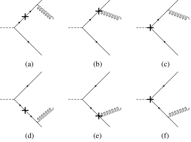
Figure 2: Counterterm diagrams to $Z\to Q{\bar{Q}}g$.

The ‘mass counterterm’ shown in the diagrams a, d is given by

$$i((Z_{\Psi}-1)k\!\!\!/-(Z_{0}-1)m_{R})\equiv i(\delta Z_{\Psi}k\!\!\!/-\delta Z_{0}m_{R})=i\delta Z_{\Psi}(k\!\!\!/-m_{R})+i(\delta Z_{\Psi}-\delta Z_{0})m_{R},$$ (III.25)

with the momentum counted in the direction of the fermion flow. The first term will result in contributions proportional to the tree amplitude, while the second term will generate a new structure which is not proportional to the tree amplitude. This term should not contain infrared divergences. Inserting the explicit results for $\delta Z_{\Psi}$, and $\delta Z_{0}$ it can be easily checked that this term is indeed IR finite. The other contribution from the remaining counterterms (diagrams b, c, e, f) are proportional to the tree amplitude. Using the relation $Z_{g}=(Z_{A})^{-1/2}$ [36] valid in the background field gauge as long as one uses the MS or $\overline{{\rm MS}}$ scheme for the gluon field and coupling, we find that the gluon renormalization enters only through the residue ${\cal Z}_{A}$ of the renormalized gluon propagator. The contribution from the counterterms is thus given by

$$(2\delta Z_{\Psi}-\delta Z_{\Psi}){\cal T}^{\mbox{\scriptsize tree}}+\tilde{\cal T}^{\mbox{\scriptsize ct, a+d}}=\delta Z_{\Psi}{\cal T}^{\mbox{\scriptsize tree}}+\tilde{\cal T}^{\mbox{\scriptsize ct, a+d}}$$ (III.26)

with $\tilde{\cal T}^{\mbox{\scriptsize ct, a+d}}$ the contribution from the insertion of $i(\delta Z_{\Psi}-\delta Z_{0})m_{R}$. For the squared amplitude we get

$$2\delta Z_{\Psi}h_{6}^{\mbox{\scriptsize LO}}-32\*\pi\alpha_{s}(N^{2}-1)(\delta Z_{\Psi}-\delta Z_{0})\*\delta h_{6}.$$ (III.27)

In the on-shell scheme we have

$$\delta Z_{\Psi}^{\mbox{\scriptsize on}} = {\alpha_{s}\over 4\*\pi}\*r_{\Gamma}\*C_{F}\left({m^{2}\over 4\*\pi\*\mu^{2}}\right)^{-\epsilon}\*\left\{-{1\over\epsilon}+{2\over\epsilon_{\mbox{\scriptsize IR}}}-4\right\}+O(\epsilon)$$ (III.28)

and

$$\delta Z_{\Psi}^{\mbox{\scriptsize on}}-\delta Z_{0}^{\mbox{\scriptsize on}} = {\alpha_{s}\over 4\*\pi}\*C_{F}r_{\Gamma}\left({m^{2}\over 4\pi\mu^{2}}\right)^{-\epsilon}\left\{{3\over\epsilon}+4\right\}+O(\epsilon).$$ (III.29)

To distinguish between infrared and ultraviolet singularities we have introduced $\epsilon_{\mbox{\scriptsize IR}}$ by $d=4+2\epsilon_{\mbox{\scriptsize IR}}$. This allows us to check separately the cancellation of the UV and IR singularities. To finish the renormalization procedure we must include the contribution from the residue of the gluon propagator ${\cal Z}_{A}^{\overline{{\rm MS}}}$:

$$({\cal Z}_{A}^{\overline{{\rm MS}}})^{{1\over 2}}{\cal T}^{\mbox{\scriptsize tree}}$$ (III.30)

which amounts to

$$2(({\cal Z}_{A}^{\overline{{\rm MS}}})^{1/2}-1)|{\cal T}^{\mbox{\scriptsize tree}}|^{2}$$ (III.31)

at the level of the squared matrix element. (In the on-shell scheme the residue ${\cal Z}_{\Psi}$ of the renormalized quark propagator is one by definition.) We have

$${\cal Z}_{A}^{\overline{{\rm MS}}} = 1-{\alpha_{s}\over 4\*\pi}\*{1\over 3}{\left(4\pi\right)^{\epsilon}\over\Gamma(1-\epsilon)}\Big{[}{1\over\epsilon_{\mbox{\scriptsize IR}}}\*(2\*n_{f}^{l}-11\*N)-2\*\sum_{i}\ln{m_{i}^{2}\over\mu^{2}}\Big{]}+O(\epsilon)\equiv 1-\delta{\cal Z}_{A}^{\overline{{\rm MS}}},$$ (III.32)

where $n_{f}^{l}$ is the number of massless flavours and the $m_{i}$ are the masses of the massive quarks, including the flavour of eq. (II.1), that contribute to the gluon self energy. We can now write down the entire contribution from UV renormalization:

$$\left.h_{6}^{\mbox{\scriptsize virt., ren.}}\right|_{\mbox{\scriptsize UV}} = (2\delta Z_{\Psi}^{\mbox{\scriptsize on}}-\delta{\cal Z}_{A}^{\overline{{\rm MS}}})h_{6}^{\mbox{\scriptsize LO}}-32\*\pi\alpha_{s}(N^{2}-1)(\delta Z_{\Psi}^{\mbox{\scriptsize on}}-\delta Z_{0}^{\mbox{\scriptsize on}})\*\delta h_{6}$$

$$= -{\alpha_{s}\over 2\*\pi}\*r_{\Gamma}\*C_{F}\left({m^{2}\over 4\pi\mu^{2}}\right)^{-\epsilon}\*{1\over\epsilon}h_{6}^{\mbox{\scriptsize LO}}-24\alpha_{s}^{2}(N^{2}-1)C_{F}r_{\Gamma}\left({m^{2}\over 4\pi\mu^{2}}\right)^{-\epsilon}{1\over\epsilon}\*\delta h_{6}$$

$$+ {\alpha_{s}\over 4\*\pi}\*r_{\Gamma}\*\left({m^{2}\over 4\pi\mu^{2}}\right)^{-\epsilon}{1\over\epsilon_{\mbox{\scriptsize IR}}}\left\{4C_{F}-{1\over 3}\*\left(2\*n_{f}^{l}-11\*N\right)\right\}h_{6}^{\mbox{\scriptsize LO}}$$

$$+ {\alpha_{s}\over 4\*\pi}\*\left\{{1\over 3}\*(2\*n_{f}-11\*N)\ln({m^{2}\over\mu^{2}})+{2\over 3}\*\sum_{i}\ln{m_{i}^{2}\over m^{2}}-8C_{F}\right\}h_{6}^{\mbox{\scriptsize LO}}-32\alpha_{s}^{2}(N^{2}-1)C_{F}\delta h_{6}.$$

Comparing this result with eq. (III.10) it follows immediately that all the UV singularities cancel. In addition it can be seen that the factor $\mu^{2\epsilon}$ in front of the UV singularities cancels together with the singularities. As we will show in section IV.3 the same is true for the $\mu$-dependence in front of the IR singularities. The remaining $\mu$-dependence is thus given by

$${\alpha_{s}\over 4\*\pi}\*\beta_{0}\ln({\mu^{2}\over m^{2}})h_{6}^{\mbox{\scriptsize LO}}\quad\mbox{with}\quad\beta_{0}={1\over 3}\*(11\*N-2\*n_{f})$$ (III.34)

as it should be according to the renormalization group equation. However this is only true as long as we renormalize the mass parameter in the on-shell scheme.

We close this subsection with some remarks concerning the treatment of $\gamma_{5}$. Since we perform the computation of $h_{6}$ in $d$ dimensions, we have to give a prescription how to treat $\gamma_{5}$. We use the following substitution in the axial vector current (remember that $\mu$ is a 4-dimensional index) [32, 33]:

$$\gamma_{\mu}\gamma_{5}\rightarrow Z_{5}^{ns}\frac{i}{3!}\,\varepsilon_{\mu\beta\gamma\delta}\,\gamma^{\beta}\gamma^{\gamma}\gamma^{\delta},\qquad\mbox{with}\quad Z_{5}^{ns}=1-\frac{\alpha_{s}}{\pi}C_{F}+{\cal O}(\alpha_{s}^{2}).$$ (III.35)

The finite ‘counterterm’ $(Z_{5}^{ns}-1)$ induces a contribution

$$\left.h_{6}^{\mbox{\scriptsize virt., ren.}}\right|_{{\gamma_{5}}}=-\frac{\alpha_{s}}{\pi}C_{F}h_{6}^{\mbox{\scriptsize LO}}.$$ (III.36)

This term is necessary to restore the chiral Ward identities, which can be checked in the present case by verifying the following relation:

$$h_{6}^{VA}(m=0)=h_{6}^{AV}(m=0).$$ (III.37)

Here, the index ${VA}({AV})$ denotes the contribution to $h_{6}$ from the interference of the Born (1-loop) vector current with the 1-loop (Born) axial vector current. We have checked that after inclusion of the term given in eq. (III.36) the relation shown in eq. (III.37) is indeed satisfied.

III.5 Checks of the calculation

The finite parts of the loop contributions to the virtual corrections are given by the rather complicated expressions eq. (III.3) and eq. (III.3). It is important to perform some checks to ensure their correctness. To this end it is useful to realize that the decomposition in terms of (coefficients)$\times$(one-loop integrals) is unique in the sense that in the massless case the coefficients of the loop-integrals can be uniquely reconstructed from the coefficients of specific logarithms even after having inserted the analytic expressions for the loop-integrals.

Most of the coefficients are highly constrained due to the general properties of infrared finiteness and renormalizability. As already mentioned above, only the $A$ and $B_{0}$ integrals contain UV singularities. Therefore the fact that all UV singularities cancel after inclusion of the counterterms is an excellent check of the coefficients of the one- and two-point integrals, which are each quite involved but combine to give the rather simple expression eq. (III.10). As discussed in section III.2, all IR singularities reside in three-point integrals. They are given explicitly in eq. (III.16) and eq. (III.20). Therefore the coefficients of the IR divergent $C_{0}$ integrals are constrained by the requirement that the IR singularities in the virtual corrections cancel against the IR singularities from the real emission processes. We will see in the next section that this cancellation really takes place (cf. eq. (IV.33) and eq. (IV.34)). Note that only the coefficients of the IR finite $C_{0}$ integrals are not tested by the consideration above. (The coefficients of the box-integrals enter the coefficients of the divergent $C_{0}$ integrals and are thus also tested.) Since all coefficients of the loop integrals are computed simultaneously by one code, the above considerations provide already a quite powerful check.

We can, however, perform an additional test by comparing our result in the limit $m\to 0$ with the known massless result for $h_{6}$ given in references [29, 30], and [31]. In these references the loop-integrals are substituted by their analytic expressions in terms of logarithms and dilogarithms. As mentioned above we can reconstruct the coefficients of the loop-integrals from the coefficients of specific logarithms and dilogarithms. For example in the massless case the dilogarithm appears only in the box-integrals. As a consequence the coefficient of the function $r(x,y)$ defined in eq. (4.11) of ref. [30] must be proportional to the coefficients of the box-integrals in our result, if we consider the massless case. Note that the massless case cannot be derived by simply taking the massless limit, because the massless limit of the loop-integrals does not exist in general. However we can still compare the coefficients of the loop integrals with the massless result by setting $z=0$ in the coefficients and checking which logarithm/dilogarithm in the results of ref. [30] are generated from which loop-integrals if one calculates the integrals for massless quarks. We do not need to worry about the additional collinear singularities which are present in the loop-integrals for massless quarks, as long as we want to check only the coefficients of the loop-integrals.

In this way we can compare our result for example to the one given in eq. (4.9) and eq. (4.10) of ref. [30]. The definition of $H_{6,7}$ in ref. [30] differs by a factor of 2 from ours due to a different convention in the definition of the electroweak couplings. Taking this into account, we find complete agreement of our result with the coefficients of the $\ln^{2}$, $\ln$ and $r(x,y)$ functions in eq. (4.10) of ref. [30]. We also can reproduce their rational function, but only up to a multiple of the Born result. This is not surprising, since the massless limit induces additional divergent and finite terms and since we use a different method to isolate the IR divergences in the real emission processes. For the leading contribution in the number of colours we find agreement of our coefficients with those of eq. (4.9) in ref. [30] up to an overall factor $(-1)$. This is most probably caused by a typographical error which is also present in ref. [29], but not in ref. [31] with which we fully agree.

IV Singular contributions from real emission

In this section we discuss the cancellation of the soft and collinear singularities appearing in the loop corrections in particular eq. (III.16), eq. (III.20) and eq. (LABEL:eq:ren-contr). To cancel them we must include the singular contributions from the real emission processes, in particular ${e^{+}e^{-}}\to Q{\bar{Q}}q{\bar{q}}$ and ${e^{+}e^{-}}\to Q{\bar{Q}}gg$, with $q$ denoting a light quark. The reactions ${e^{+}e^{-}}\to Q{\bar{Q}}Q^{\prime}{\bar{Q}}^{\prime}$ and ${e^{+}e^{-}}\to Q{\bar{Q}}Q{\bar{Q}}$ do not yield a singular contribution. As a consequence these contributions can be integrated numerically in 4 dimensions. In ${e^{+}e^{-}}\to Q{\bar{Q}}Q^{\prime}{\bar{Q}}^{\prime},Q{\bar{Q}}Q{\bar{Q}}$ the collinear singularities which would appear for massless quarks are regulated by the quark mass and give rise to $\ln(m^{2})$ terms. To a certain extend these logarithms cancel in the sum of virtual and real contributions. On the other hand in tagged cross sections one encounters in general the situation where uncancelled logarithms remain in the final result. For example in ${e^{+}e^{-}}\to Q{\bar{Q}}q{\bar{q}}$ it can be easily seen that such logarithms will be produced when the heavy quark pair is produced by a gluon emitted from the light quarks. Due to the fact that this contribution is proportional to the couplings of the light quarks to the Z boson it can never be cancelled by the virtual contributions. In the presence of several scales of different orders of magnitude these logarithms may spoil the convergence of fixed order perturbation theory and indicate a sensitivity to long distance phenomena. (Because of these logarithms it is for example not longer possible to take the massless limit!) The uncancelled logarithms may need a treatment by renormalization group techniques which goes beyond the fixed order perturbation theory. In particular they should be absorbed into the appropriate fragmentation functions. These contributions can also be isolated by experimental cuts [39, 40, 41].

To cancel soft and collinear singularities several algorithms have been developed in the past [16, 42, 43]. In this work we use the phase space slicing method which was modified to include mass effects in $e^{+}e^{-}\to 3$ jets in references [20, 21] and generalized to treat massive quarks in arbitrary jet cross sections in ref. [18]. Here we restrict ourself to the singular parts from the real emission processes. The finite contributions which can be calculated by numerical integration of the existing leading order matrix elements will be discussed elsewhere. The idea of the phase space slicing is to split the phase space of the real emission contributions into regions where all the partons are hard and not collinear (resolved regions) and the remaining regions where two partons are collinear or a parton is soft (unresolved regions). The separation into resolved and unresolved regions can be performed by introducing appropriate Heaviside functions. In the unresolved regions one can make use of the soft and collinear factorization to approximate the matrix elements. Due to this simplifications it is possible to perform the integrations analytically over the unresolved regions.

To fix the notation and to define as clearly as possible resolved and unresolved contributions we outline in the next two sections the phase space slicing method applied to the problem at hand.

IV.1 Singular contribution from $Q\bar{Q}q\bar{q}$

The matrix element for $e^{+}e^{-}\to Q(k_{Q}){\bar{Q}}(k_{\bar{Q}})q(k_{q}){\bar{q}}(k_{\bar{q}})$ is singular in the limit $k_{q}||k_{\bar{q}}$. Defining $t_{ij}=2k_{i}\cdot k_{j}$ we may introduce the following slicing:

$$|{\cal T}(Q(k_{Q}){\bar{Q}}(k_{\bar{Q}})q(k_{q}){\bar{q}}(k_{\bar{q}}))|^{2}=[\Theta(t_{q{\bar{q}}}-s_{\mbox{\scriptsize min}})+\Theta(s_{\mbox{\scriptsize min}}-t_{q{\bar{q}}})]|{\cal T}(Q(k_{Q}){\bar{Q}}(k_{\bar{Q}})q(k_{q}){\bar{q}}(k_{\bar{q}}))|^{2},$$ (IV.1)

where $s_{\mbox{\scriptsize min}}$ denotes an arbitrary mass scale squared which separates between collinear and resolved regions. The resolved contribution

$$d\sigma_{R}=\Theta(t_{Q{\bar{Q}}}-s_{\mbox{\scriptsize min}})|{\cal T}(Q(k_{Q}){\bar{Q}}(k_{\bar{Q}})q(k_{q}){\bar{q}}(k_{\bar{q}}))|^{2}dR^{d}(k_{Q},k_{\bar{Q}},k_{q},k_{\bar{q}})$$ (IV.2)

is free of collinear singularities and can thus be integrated numerically in 4 dimensions.
Here $dR^{d}(k_{Q},k_{\bar{Q}},k_{q},k_{\bar{q}})$ denotes the four particle phase space measure in $d$ dimensions:

$$dR^{d}(k_{1},\ldots,k_{n})={1\over{\cal N}}(2\pi)^{d}\delta^{(d)}(K-\sum_{i=1}^{n}k_{i})\prod_{i=1}^{n}{d^{d-1}k_{i}\over(2\pi)^{d-1}2k_{i}^{0}}.$$ (IV.3)

(${\cal N}$ is a symmetry factor.) For small $s_{\mbox{\scriptsize min}}$ the second term in eq. (IV.1) can be approximated using the factorization of amplitudes in the collinear limit:

$$\Theta(s_{\mbox{\scriptsize min}}-t_{q{\bar{q}}})|{\cal T}(Q(k_{Q}){\bar{Q}}(k_{\bar{Q}})q(k_{q}){\bar{q}}(k_{\bar{q}}))|^{2}$$ (IV.4)

$$\stackrel{{\scriptstyle k_{q}||k_{\bar{q}}}}{{\longrightarrow}} \Theta(s_{\mbox{\scriptsize min}}-t_{q{\bar{q}}})|{\cal T}(Q(k_{Q}){\bar{Q}}(k_{\bar{Q}})g(k_{q}+k_{\bar{q}}))|^{2}g_{s}^{2}{2\over t_{q{\bar{q}}}}P_{q{\bar{q}}\to g}(z)$$

where $P_{g\to q{\bar{q}}}(z)$ is the Altarelli-Parisi kernel [44] (in conventional dimensional regularization)

$$P_{q{\bar{q}}\to g}(z)={1\over 2}{z^{2}+(1-z)^{2}-\epsilon\over 1-\epsilon}$$ (IV.5)

and $z$ denotes the momentum fraction in the collinear limit:

$$k_{q}=z(k_{q}+k_{\bar{q}}).$$ (IV.6)

Using in addition the factorization of the phase-space measure in the collinear limit [16]:

$$dR^{d}(k_{Q},k_{\bar{Q}},k_{q},k_{\bar{q}})\stackrel{{\scriptstyle k_{q}||k_{\bar{q}}}}{{\longrightarrow}}dR^{d}(k_{Q},k_{\bar{Q}},P)dR_{\mbox{\scriptsize coll.}}(k_{q},k_{\bar{q}})$$ (IV.7)

with

$$dR_{\mbox{\scriptsize coll.}}(k_{q},k_{\bar{q}})={1\over 16\*\pi^{2}}\*{\left({4\*\pi\mu^{2}}\right)^{\epsilon}\over\Gamma(1-\epsilon)}\*\,dt_{q{\bar{q}}}dz[t_{q{\bar{q}}}z(1-z)]^{-\epsilon}$$ (IV.8)

the unresolved contribution to the cross section after integration over the collinear region is given by

$$d\sigma_{U}(Q(k_{Q}){\bar{Q}}(k_{\bar{Q}})q(k_{q}){\bar{q}}(k_{\bar{q}}))=d\sigma(Q(k_{Q}){\bar{Q}}(k_{\bar{Q}})g(k_{g})){\cal C}_{q{\bar{q}}}$$ (IV.9)

with

$${\cal C}_{q{\bar{q}}} = -{g_{s}^{2}\over 8\*\pi^{2}}\*{1\over\Gamma(1-\epsilon)}\*\left({4\*\pi\mu^{2}\over s_{\mbox{\scriptsize min}}}\right)^{\epsilon}{1\over\epsilon}\int_{0}^{1}dz[z(1-z)]^{-\epsilon}P_{q{\bar{q}}\to g}(z)$$ (IV.10)

$$= -{\alpha_{s}\over 2\*\pi}\*{1\over\Gamma(1-\epsilon)}\*\left({4\*\pi\mu^{2}\over s_{\mbox{\scriptsize min}}}\right)^{\epsilon}{1\over\epsilon}\*{1-\epsilon\over 3-2\*\epsilon}\*{\Gamma^{2}(1-\epsilon)\over\Gamma(2-2\*\epsilon)}.$$

In eq. (IV.9) we have identified the sum of momenta $k_{q}+k_{\bar{q}}$ with the momentum $k_{g}$ of the outgoing ‘recombined’ gluon. In particular the singular contribution to $h_{6}$ is given by ${\cal C}_{q{\bar{q}}}\times h_{6}^{\mbox{\scriptsize LO}}.$ We get the same contribution for each massless quark flavour. This results to an overall factor $n_{f}^{l}$ with $n_{f}^{l}$ the number of light flavours.

IV.2 Singular contribution from $Q\bar{Q}gg$

The singular behavior of the matrix element for ${e^{+}e^{-}}\to Q(k_{Q}){\bar{Q}}(k_{\bar{Q}})g(k_{1})g(k_{2})$ is far more complicated than that discussed in the previous section. While in ${e^{+}e^{-}}\to Q{\bar{Q}}q{\bar{q}}$ only collinear singularities appear we have now both: soft and collinear singularities. In addition only the colour ordered sub-amplitudes show a simple factorization in the soft limit. So we may start with the colour decomposition of the amplitude which reads

$${\cal T}(Q(k_{Q}){\bar{Q}}(k_{\bar{Q}})g(k_{1})g(k_{2}))=(T_{a_{1}}T_{a_{2}})_{c_{Q}c_{\bar{Q}}}S_{1}+(T_{a_{2}}T_{a_{1}})_{c_{Q}c_{\bar{Q}}}S_{2}.$$ (IV.11)

Here $c_{Q}$ ($c_{\bar{Q}}$) is the colour index of the (anti-) quark, and $a_{1}$, $a_{2}$ are the colour indices of the gluons. In our conventions the colour matrices satisfy $\mbox{\sf Tr}[T_{a}T_{b}]=\delta_{ab}$. The amplitudes $S_{1}$, $S_{2}$ are the so called colour ordered sub-amplitudes. The squared amplitude in terms of the sub-amplitudes is given by

$$\sum_{\mbox{\scriptsize colour}}|{\cal T}(Q(k_{Q}){\bar{Q}}(k_{\bar{Q}})g(k_{1})g(k_{2}))|^{2}=(N^{2}-1)\*\left(N\*(|S_{1}|^{2}+|S_{2}|^{2})-{1\over N}|S_{1}+S_{2}|^{2}\right).$$ (IV.12)

Note that the sub-amplitudes are gauge independent. We can thus study the soft and collinear limits independently for $|S_{1}|^{2}$, $|S_{2}|^{2}$ and $|S_{1}+S_{2}|^{2}$. The contribution $|S_{1}+S_{2}|^{2}$ is essentially QED-like. It is therefore free of collinear singularities in the limit that the two gluons become collinear. The amplitude $S_{2}$ can be obtained from $S_{1}$ by exchanging the two gluon momenta. So let us start with the treatment of $S_{1}$. The appropriate invariants for the phase space slicing are $t_{Q1}$, $t_{12}$ and $t_{2{\bar{Q}}}$. We start with the following identity:

$$1 = [\Theta(t_{Q1}-s_{\mbox{\scriptsize min}})+\Theta(s_{\mbox{\scriptsize min}}-t_{Q1})]\*[\Theta(t_{12}-s_{\mbox{\scriptsize min}})+\Theta(s_{\mbox{\scriptsize min}}-t_{12})]$$ (IV.13)

$$\times[\Theta(t_{2{\bar{Q}}}-s_{\mbox{\scriptsize min}})+\Theta(s_{\mbox{\scriptsize min}}-t_{2{\bar{Q}}})]$$

$$= \Theta(t_{Q1}-s_{\mbox{\scriptsize min}})\*\Theta(t_{12}-s_{\mbox{\scriptsize min}})\*\Theta(t_{2{\bar{Q}}}-s_{\mbox{\scriptsize min}})$$

$$+ \Theta(t_{Q1}-s_{\mbox{\scriptsize min}})\*\Theta(s_{\mbox{\scriptsize min}}-t_{12})\*\Theta(t_{2{\bar{Q}}}-s_{\mbox{\scriptsize min}})\mbox{ 1,2 collinear}$$

$$+ \Theta(t_{Q1}-s_{\mbox{\scriptsize min}})\*\Theta(s_{\mbox{\scriptsize min}}-t_{12})\*\Theta(s_{\mbox{\scriptsize min}}-t_{2{\bar{Q}}})\mbox{ 2 soft}$$

$$+ \Theta(s_{\mbox{\scriptsize min}}-t_{Q1})\*\Theta(s_{\mbox{\scriptsize min}}-t_{12})\*\Theta(t_{2{\bar{Q}}}-s_{\mbox{\scriptsize min}})\mbox{ 1 soft}$$

$$+ \Theta(t_{Q1}-s_{\mbox{\scriptsize min}})\*\Theta(t_{12}-s_{\mbox{\scriptsize min}})\*\Theta(s_{\mbox{\scriptsize min}}-t_{2{\bar{Q}}})\mbox{ {$\bar{Q}$},2 collinear}$$

$$+ \Theta(s_{\mbox{\scriptsize min}}-t_{Q1})\*\Theta(t_{12}-s_{\mbox{\scriptsize min}})\*\Theta(t_{2{\bar{Q}}}-s_{\mbox{\scriptsize min}})\mbox{ Q,1 collinear}$$

$$+ \Theta(s_{\mbox{\scriptsize min}}-t_{Q1})\*\Theta(t_{12}-s_{\mbox{\scriptsize min}})\*\Theta(s_{\mbox{\scriptsize min}}-t_{2{\bar{Q}}})\mbox{ Q,1 collinear and {$\bar{Q}$},2 collinear}$$

$$+ \Theta(s_{\mbox{\scriptsize min}}-t_{Q1})\*\Theta(s_{\mbox{\scriptsize min}}-t_{12})\*\Theta(s_{\mbox{\scriptsize min}}-t_{2{\bar{Q}}})\mbox{ 1 and 2 soft}$$

The first line in the decomposition above corresponds to the resolved region: both gluons are hard and not collinear to each other. Combined with the squared matrix element this contribution can be integrated numerically in 4 dimensions. The next three lines describe the single unresolved regions which yield a singular contribution after phase space integration. There are also single unresolved contributions when one of the two gluons becomes ‘collinear’ to the heavy quark or anti-quark. These contributions do not yield a singular contribution after phase space integration, because of the mass of the quarks. In principle they should be of order $s_{\mbox{\scriptsize min}}$. In fact for small enough values for $s_{\mbox{\scriptsize min}}$ these contributions vanish, because the quark mass serves already as a cutoff. This can be checked by including them in the numerical integration procedure. The last two lines describe ‘double unresolved’ contributions. As long as we restrict ourself to three-jet quantities, these terms do not contribute. The above slicing of the phase space differs slightly from the one used in our previous work [20, 21] and corresponds to the one used in ref. [18]. For the leading colour contributions the slicing (IV.13) is more convenient than the one used in references [20, 21], because the soft factor (see below) is more compact and the separation of soft and collinear regions is simpler, facilitating the numerical implementation. We have checked numerically that the two slicing methods are equivalent.

Let us now discuss the contributions from the soft regions, for example the region where momentum $k_{1}$ is ‘soft’:

$$\delta d\sigma_{U}=\Theta(s_{\mbox{\scriptsize min}}-t_{Q1})\*\Theta(s_{\mbox{\scriptsize min}}-t_{12})\*\Theta(t_{2{\bar{Q}}}-s_{\mbox{\scriptsize min}})|S_{1}|^{2}dR^{d}(k_{Q},k_{\bar{Q}},k_{1},k_{2})$$ (IV.14)

Using the soft factorization of the squared matrix element

$$N(N^{2}-1)|S_{1}|^{2}\stackrel{{\scriptstyle\mbox{\scriptsize 1 soft}}}{{\longrightarrow}}g_{s}^{2}\frac{N}{2}f(k_{Q},k_{1},k_{2})|{\cal T}(Q(k_{Q}){\bar{Q}}(k_{\bar{Q}})g(k_{2}))|^{2}$$ (IV.15)

with

$$f(k_{i},k_{s},k_{j})={4\,t_{ij}\over t_{is}t_{sj}}-{4\,k_{i}^{2}\over t_{is}^{2}}-{4\,k_{j}^{2}\over t_{js}^{2}},$$ (IV.16)

together with the soft factorization of the phase space measure

$$dR^{d}(k_{Q},k_{\bar{Q}},k_{1},k_{2})\to dR^{d}(k_{Q},k_{\bar{Q}},k_{2}){1\over 2}dR_{\mbox{\scriptsize soft}}$$ (IV.17)

(the factor 1/2 is the symmetry factor for the two identical gluons) we arrive at

$$\delta d\sigma_{U}=\frac{N}{2}S(m,0,t_{Q2})|{\cal T}(Q(k_{Q}){\bar{Q}}(k_{\bar{Q}})g(k_{2}))|^{2}dR^{d}(k_{Q},k_{\bar{Q}},k_{2})$$ (IV.18)

with

$$S(m_{i},m_{j},t_{ij})={g_{s}^{2}\over 2}\int dR_{\mbox{\scriptsize soft}}f(k_{i},k_{s},k_{j})\Theta(s_{\mbox{\scriptsize min}}-t_{is})\Theta(s_{\mbox{\scriptsize min}}-t_{sj}),\quad\mbox{for}\quad k_{i}^{2}=m_{i}^{2}.$$ (IV.19)

Explicitly [18],

$$S(m,0,t_{Q2}) = \frac{\alpha_{s}}{2\pi}\frac{1}{\Gamma(1-\epsilon)}\left(\frac{4\pi\mu^{2}}{s_{\mbox{\scriptsize min}}}\right)^{\epsilon}\left(\frac{t_{Q2}}{s_{\mbox{\scriptsize min}}}\right)^{\epsilon}J(m,0,t_{Q2}),$$ (IV.20)

where

$$J(m,0,t_{Q2}) = \Theta(t_{Q2}-m^{2})\left[\frac{1}{\epsilon^{2}}-\frac{1}{2\epsilon^{2}}\left(\frac{t_{Q2}}{m^{2}}\right)^{\epsilon}+\frac{1}{2\epsilon}\left(\frac{t_{Q2}}{m^{2}}\right)^{\epsilon}-\frac{1}{2}\zeta(2)+\frac{m^{2}}{t_{Q2}}\right]$$ (IV.21)

$$+ \Theta(m^{2}-t_{Q2})\left(\frac{t_{Q2}}{m^{2}}\right)^{-\epsilon}\left[\frac{1}{2\epsilon^{2}}+\frac{1}{2\epsilon}-\frac{1}{2}\zeta(2)+1\right].$$

The case that gluon 2 becomes soft can be treated in the same way. To finish our discussion of the singular contribution from $S_{1}$ let us discuss the contribution from the collinear region. Here the same procedure as in the massless case applies. For details we refer to the previous section or to ref. [16]. So we quote only the final result:

$$\Theta(t_{Q1}-s_{\mbox{\scriptsize min}})\*\Theta(s_{\mbox{\scriptsize min}}-t_{12})\*\Theta(t_{2{\bar{Q}}}-s_{\mbox{\scriptsize min}})|S_{1}|^{2}dR^{d}(k_{Q},k_{\bar{Q}},k_{1},k_{2})$$ (IV.22)

$$\approx N{\cal C}_{gg}|{\cal T}(Q(k_{Q}){\bar{Q}}(k_{\bar{Q}})g(k_{g}))|^{2}dR^{d}(k_{Q},k_{\bar{Q}},k_{g})$$

with

$${\cal C}_{gg} = -{1\over 2}{g_{s}^{2}\over 16\*\pi^{2}}\*{1\over\Gamma(1-\epsilon)}\*\left({4\*\pi\mu^{2}\over s_{\mbox{\scriptsize min}}}\right)^{\epsilon}{1\over\epsilon}\int_{z_{1}}^{1-z_{2}}dz[z(1-z)]^{-\epsilon}P_{gg\to g}(z)$$ (IV.23)

$$= -{\alpha_{s}\over 2\*\pi}\*{1\over\Gamma(1-\epsilon)}\*\left({4\*\pi\mu^{2}\over s_{\mbox{\scriptsize min}}}\right)^{\epsilon}{1\over\epsilon}I_{gg\to g},$$

and

$$I_{gg\to g} = {(z_{Q})^{-\epsilon}\over\epsilon}+{(z_{\bar{Q}})^{-\epsilon}\over\epsilon}-{3\*(1-\epsilon)\*(4-3\*\epsilon)\over 2\*\epsilon\*(3-2\*\epsilon)}\*{\Gamma(1-\epsilon)^{2}\over\Gamma(2-2\*\epsilon)}$$

where $z_{Q}$ and $z_{\bar{Q}}$ are defined as follows:

$$z_{Q}={s_{\mbox{\scriptsize min}}\over t_{Qg}},\qquad z_{\bar{Q}}={s_{\mbox{\scriptsize min}}\over t_{{\bar{Q}}g}}.$$ (IV.25)

For $|S_{2}|^{2}$ we may apply the same procedure as for $|S_{1}|^{2}$. The soft singularities appearing in $|S_{1}+S_{2}|^{2}$ can be treated in a similar way as the singularities in $S_{1}$. Since the amplitude $S_{1}+S_{2}$ is a QED-like contribution with massive quarks, it does not induce collinear singularities. The soft singularities can be isolated most easily by using the following identity:

$$1=[\Theta(s_{\mbox{\scriptsize min}}-t_{Q1}-t_{{\bar{Q}}1})+\Theta(t_{Q1}+t_{{\bar{Q}}1}-s_{\mbox{\scriptsize min}})]\*[\Theta(s_{\mbox{\scriptsize min}}-t_{Q2}-t_{{\bar{Q}}2})+\Theta(t_{Q2}+t_{{\bar{Q}}2}-s_{\mbox{\scriptsize min}})].$$ (IV.26)

If we expand this expression we obtain

$$1 = -\Theta(s_{\mbox{\scriptsize min}}-t_{Q1}-t_{{\bar{Q}}1})\*\Theta(s_{\mbox{\scriptsize min}}-t_{Q2}-t_{{\bar{Q}}2})$$ (IV.27)

$$+ \Theta(s_{\mbox{\scriptsize min}}-t_{Q1}-t_{{\bar{Q}}1})+\Theta(s_{\mbox{\scriptsize min}}-t_{Q2}-t_{{\bar{Q}}2})$$

$$+ \Theta(t_{Q1}+t_{{\bar{Q}}1}-s_{\mbox{\scriptsize min}})\*\Theta(t_{Q2}+t_{{\bar{Q}}2}-s_{\mbox{\scriptsize min}})$$

The first term describes a double unresolved contribution: both gluons must be soft to satisfy the Heaviside functions. This term does not contribute to a three-jet observable. The next two terms describe the situation in which gluon 1 or gluon 2 is soft. It is still allowed that both gluons are soft, this explains the minus sign in the first line that avoids over-counting. The last term denotes the resolved contribution which can be calculated numerically in 4 dimensions. Using the slicing given in eq. (IV.27) we thus obtain for the soft contribution from $|S_{1}+S_{2}|$:

$$[\Theta(s_{\mbox{\scriptsize min}}-t_{Q1}-t_{{\bar{Q}}1})+\Theta(s_{\mbox{\scriptsize min}}-t_{Q2}-t_{{\bar{Q}}2})](-{1\over N})(N^{2}-1)|S_{1}+S_{2}|^{2}dR^{d}(k_{Q},k_{\bar{Q}},k_{1},k_{2})$$

$$\to-{1\over N}S(m,m,t_{Q{\bar{Q}}})|{\cal T}(Q(k_{Q}){\bar{Q}}(k_{\bar{Q}})g(k_{g}))|^{2}dR^{d}(k_{Q},k_{\bar{Q}},k_{g})$$ (IV.28)

where we have used the factorization in the soft region which now takes the form:

$$-{1\over N}\*(N^{2}-1)\*|S_{1}+S_{2}|^{2}\stackrel{{\scriptstyle\mbox{\scriptsize 1 soft}}}{{\longrightarrow}}-{1\over 2N}g_{s}^{2}f(k_{Q},k_{1},k_{\bar{Q}})|{\cal T}(Q(k_{Q}){\bar{Q}}(k_{\bar{Q}})g(k_{g}))|^{2}.$$ (IV.29)

Note that we have once again identified the momentum of the remaining hard gluon with $k_{g}$. The explicit result for $S(m,m,t_{Q{\bar{Q}}})$ is [21]

$$S(m,m,t_{Q{\bar{Q}}})={\alpha_{s}\over 2\pi}{1\over\Gamma(1-\epsilon)}\left({4\pi\mu^{2}\over s_{\mbox{\scriptsize min}}}\right)^{\epsilon}\left({t_{Q{\bar{Q}}}+2\*m^{2}\over s_{\mbox{\scriptsize min}}}\right)^{\epsilon}J(m,m,t_{Q{\bar{Q}}}),$$ (IV.30)

where

$$J(m,m,t_{Q{\bar{Q}}})={1\over\epsilon}-{1+\omega\over 1-\omega}\ln(\omega)+{1+\omega^{2}\over 1-\omega^{2}}\left\{{1\over\epsilon}\*\ln(\omega)-{1\over 2}\*\ln^{2}(\omega)-2\,{{\rm Li}_{2}}(1-\omega)\right\}+O(\epsilon)$$ (IV.31)

and $\omega$ was defined in (III.19). Combining all singular contributions from $|S_{1}|^{2}$, $|S_{2}|^{2}$, and $|S_{1}+S_{2}|^{2}$ we obtain the following result for the unresolved contribution:

$$\left\{NS(m,0,t_{Qg})+NS(m,0,t_{{\bar{Q}}g})+N{\cal C}_{gg\to g}-{1\over N}S(m,m,t_{Q{\bar{Q}}})\right\}d\sigma(Q(k_{Q}){\bar{Q}}(k_{\bar{Q}})g(k_{g}))$$ (IV.32)

$$= {\alpha_{s}\over 2\pi}{1\over\Gamma(1-\epsilon)}\left({4\pi\mu^{2}\over s_{\mbox{\scriptsize min}}}\right)^{\epsilon}\times\Bigg{\{}N\left[\left({t_{Qg}\over s_{\mbox{\scriptsize min}}}\right)^{\epsilon}J(m,0,t_{Qg})+\left({t_{{\bar{Q}}g}\over s_{\mbox{\scriptsize min}}}\right)^{\epsilon}J(m,0,t_{{\bar{Q}}g})-{1\over\epsilon}I_{gg\to g}\right]$$

$$- {1\over N}\left({t_{Q{\bar{Q}}}+2\*m^{2}\over s_{\mbox{\scriptsize min}}}\right)^{\epsilon}J(m,m,t_{Q{\bar{Q}}})\Bigg{\}}d\sigma(Q(k_{Q}){\bar{Q}}(k_{\bar{Q}})g(k_{g}))$$

To get the singular (unresolved) contribution to $h_{6}$ one has simply to replace $d\sigma(Q(k_{Q}){\bar{Q}}(k_{\bar{Q}})g(k_{g}))$ by $h_{6}^{\mbox{\scriptsize LO}}$. Note that both quantities $d\sigma(Q(k_{Q}){\bar{Q}}(k_{\bar{Q}})g(k_{g}))$ and $h_{6}^{\mbox{\scriptsize LO}}$ are evaluated in $d$ dimensions. As we will show in the next subsection the same structure is obtained from the virtual corrections. After the cancellation of the IR singularities we thus need $d\sigma(Q(k_{Q}){\bar{Q}}(k_{\bar{Q}})g(k_{g}))$ or equivalently $h_{6}^{\mbox{\scriptsize LO}}$ only in 4 dimensions.

IV.3 Infrared and collinear finiteness

We close this section by demonstrating that the singular contributions discussed in the previous subsections indeed cancel the singularities encountered in the virtual corrections.

Combining eq. (III.16), eq. (III.20), and eq. (LABEL:eq:ren-contr) we obtain for the IR singularities of the virtual corrections the following result:

$$h_{6}^{\mbox{\scriptsize virt., IR div.}} = {\alpha_{s}\over 2\*\pi}\*r_{\Gamma}\left({4\*\pi\*\mu^{2}\over m^{2}}\right)^{\epsilon}\Bigg{\{}-N\left[{1\over\epsilon^{2}}-{1\over\epsilon}\*\ln({t_{Qg}\over m^{2}})-{1\over\epsilon}\*\ln({t_{{\bar{Q}}g}\over m^{2}})\right]$$ (IV.33)

$$+{1\over N}{1\over\epsilon}\*{1+\omega^{2}\over 1-\omega^{2}}\*\ln(\omega)-{1\over\epsilon}\left[2C_{F}-{1\over 6}\*(2\*n_{f}^{l}-11\*N)\right]\Bigg{\}}\*h_{6}^{\mbox{\scriptsize LO}}$$

The singular parts of the real emission processes are given by (eq. (IV.9), eq. (IV.32)):

$$\left.h_{6}^{\mbox{\scriptsize real, unres.}}\right|_{\mbox{\scriptsize div}} = {\alpha_{s}\over 2\pi}{1\over\Gamma(1-\epsilon)}\left({4\pi\mu^{2}\over m^{2}}\right)^{\epsilon}$$ (IV.34)

$$\times \Bigg{\{}N\left[{1\over\epsilon^{2}}-{1\over\epsilon}\ln\left({t_{Qg}\over m^{2}}\right)-{1\over\epsilon}\ln\left({t_{{\bar{Q}}g}\over m^{2}}\right)\right]$$

$$-{1\over N}{1\over\epsilon}{1+\omega^{2}\over 1-\omega^{2}}\*\ln(\omega)+{1\over\epsilon}\*\left[2C_{F}-{1\over 6}\*(2n_{f}^{l}-11N)\right]\Bigg{\}}\*h_{6}^{\mbox{\scriptsize LO}},$$

where we have used the expansions

$$\left({t_{Qg}\over s_{\mbox{\scriptsize min}}}\right)^{\epsilon}J(m,0,t_{Qg}) = {1\over 2\epsilon^{2}}+{1\over 2\epsilon}-{1\over 2\epsilon}\ln\left({s_{\mbox{\scriptsize min}}\over m^{2}}\right)+j(m,0,t_{Qg})+O(\epsilon)$$

$$\left({t_{Q{\bar{Q}}}+2\*m^{2}\over s_{\mbox{\scriptsize min}}}\right)^{\epsilon}J(m,m,t_{Q{\bar{Q}}}) = {1\over\epsilon}+{1\over\epsilon}\*{1+\omega^{2}\over 1-\omega^{2}}\*\ln(\omega)+j(m,m,t_{Q{\bar{Q}}})+O(\epsilon),$$

$$I_{gg\to g} = -{11\over 6}-\ln({s_{\mbox{\scriptsize min}}\over t_{Qg}})-\ln({s_{\mbox{\scriptsize min}}\over t_{{\bar{Q}}g}})$$

$$+ ({1\over 2}\*\ln^{2}({s_{\mbox{\scriptsize min}}\over t_{Qg}})+{1\over 2}\*\ln^{2}({s_{\mbox{\scriptsize min}}\over t_{{\bar{Q}}g}})+{1\over 3}\*\pi^{2}-{67\over 18})\*\epsilon+O(\epsilon^{2}),$$

$$n_{f}^{l}{1\over\epsilon}I_{q{\bar{q}}\to g} = n_{f}^{l}\*{1\over\epsilon}\*{1\over 3}+{5\over 9}n_{f}^{l}+O(\epsilon),$$ (IV.35)

with $j(m,0,t_{Qg}),j(m,m,t_{Q{\bar{Q}}})$ denoting the order 1 contributions in the expansion. They are given by

$$j(m,0,t_{Qg}) = {1\over 4}\*\ln^{2}\left({s_{\mbox{\scriptsize min}}\over m^{2}}\right)-{1\over 2}\*\ln\left({s_{\mbox{\scriptsize min}}\over m^{2}}\right)+1-{1\over 2}\zeta(2)$$ (IV.36)

$$+ \Theta(t_{Qg}-m^{2})\*\left\{-{1\over 2}\ln^{2}\left({t_{Qg}\over m^{2}}\right)+\ln\left({t_{Qg}\over m^{2}}\right)-1+{m^{2}\over t_{Qg}}\right\},$$

$$j(m,m,t_{Q{\bar{Q}}}) = \ln\left({t_{Q{\bar{Q}}}+2\*m^{2}\over s_{\mbox{\scriptsize min}}}\right)\left\{1+{1+\omega^{2}\over 1-\omega^{2}}\ln(\omega)\right\}-{1+\omega\over 1-\omega}\ln(\omega)$$ (IV.37)

$$- {1+\omega^{2}\over 1-\omega^{2}}\left\{{1\over 2}\*\ln^{2}(\omega)+2\*\,{{\rm Li}_{2}}(1-\omega)\right\}.$$

Note that we have not expanded the factor $\mu^{\epsilon}$ to show explicitly the cancellation of this factor as it was promised in section III.4. Comparing eq. (IV.33) and eq. (IV.34) one sees immediately that the singular contribution from the real corrections cancel exactly the IR divergences from the virtual corrections.

V Summary and conlusions

In this work we have calculated the virtual corrections to the parity-violating functions $F_{3}$ and $F_{6}$ of the fully differential cross section eq. (II.2) for $e^{+}e^{-}\to Q\bar{Q}g$. We have given results for the UV and IR singularities as well as for the finite contributions. We have shown explicitly the cancellation of the UV singularities after the renormalization has been performed. In addition we have calculated also the singular contribution from real corrections using the phase space slicing method. We checked that this contribution cancels exactly the IR singularities in the virtual corrections. Together with our comparison to the known results for massless quarks the cancellation of the IR and UV singularities serves as an important check of our calculation.

We have given our next-to-leading order results in terms of one function $h_{6}$, from which $F_{3}$ and $F_{6}$ can be reconstructed using eq. (II.6)–eq. (II.10). The final result for the contribution from three resolved partons, $h_{6}^{\mbox{\scriptsize 3 res., NLO}}$, can be obtained from the following formula:

$$h_{6}^{\mbox{\scriptsize 3 res., NLO}}=h_{6}^{\mbox{\scriptsize virt., fin.}}+h_{6}^{\mbox{\scriptsize rest}}+\left.h_{6}^{\mbox{\scriptsize real, unres.}}\right|_{\mbox{\scriptsize fin.}},$$ (V.1)

where $h_{6}^{\mbox{\scriptsize virt., fin.}}$ is given in eq. (III.21). The contribution $h_{6}^{\mbox{\scriptsize rest}}$ is given by

$$h_{6}^{\mbox{\scriptsize rest}} = h_{6}^{\mbox{\scriptsize virt., UV div.}}+\left.h_{6}^{\mbox{\scriptsize virt., IR div.}}\right|_{\mbox{\scriptsize lead. colour}}+\left.h_{6}^{\mbox{\scriptsize virt., IR div.}}\right|_{\mbox{\scriptsize subl. colour}}$$

$$+ \left.h_{6}^{\mbox{\scriptsize virt., ren.}}\right|_{\mbox{\scriptsize UV}}+\left.h_{6}^{\mbox{\scriptsize virt., ren.}}\right|_{{\gamma_{5}}}+\left.h_{6}^{\mbox{\scriptsize real, unres.}}\right|_{\mbox{\scriptsize div.}}$$

$$= 8\*\alpha_{s}^{2}\*(N^{2}-1)\*C_{F}\*B\*\bigg{(}1+x-2\*\bar{x}+(1-\bar{x})\*{\bar{x}\over x}$$

$$+ z\*\bigg{[}2\*B\*((\bar{x}^{2}-2\*x)\*(1-x)+(2-3\*x)\*(1-\bar{x}))+g_{1}\*{x^{2}-4\*z\over x\*(1-x)}+4\*z\*B\*(2\*{(1-\bar{x})^{2}\over 1-x}+{x_{g}})\bigg{]}\bigg{)}$$

$$+ 16\*\alpha_{s}^{2}\*C_{F}\*B\*({1\over{x_{g}}}\*(x\*\bar{x}-4\*\bar{x}+2+\bar{x}^{2})-2\*z\*{x_{g}}\*B\*(x-\bar{x}))$$

$$+ {\alpha_{s}\over 4\*\pi}\*\left\{{1\over 3}\*(2\*n_{f}-11\*N)\ln({m^{2}\over\mu^{2}})+{2\over 3}\*\sum_{i}\ln{m_{i}^{2}\over m^{2}}-8C_{F}\right\}h_{6}^{\mbox{\scriptsize LO}}-32\alpha_{s}^{2}(N^{2}-1)C_{F}\delta h_{6}-\frac{\alpha_{s}}{\pi}C_{F}h_{6}^{\mbox{\scriptsize LO}},$$

where $g_{1}$ was defined in (III.12). The finite contribution from unresolved partons is given by

$$\left.h_{6}^{\mbox{\scriptsize real, unres.}}\right|_{\mbox{\scriptsize fin.}} = {\alpha_{s}\over 2\pi}\Bigg{\{}N\bigg{[}j(m,0,t_{Qg})+j(m,0,t_{{\bar{Q}}g})-({1\over 2}\*\ln^{2}({s_{\mbox{\scriptsize min}}\over t_{Qg}})+{1\over 2}\*\ln^{2}({s_{\mbox{\scriptsize min}}\over t_{{\bar{Q}}g}})+{1\over 3}\*\pi^{2}-{67\over 18})\bigg{]}$$ (V.3)

$$- {1\over N}j(m,m,t_{Q{\bar{Q}}})-{5\over 9}n_{f}^{l}\Bigg{\}}h_{6}^{\mbox{\scriptsize LO}}.$$

The functions $j(m,0,t_{Qg})$, and $j(m,m,t_{Q{\bar{Q}}})$ are given in eq. (IV.36) and eq. (IV.37), respectively. Note that $\left.h_{6}^{\mbox{\scriptsize real, unres.}}\right|_{\mbox{\scriptsize fin.}}$ depend on the method used to combine virtual and real corrections. Furthermore we can set $d=4$ in $h_{6}^{\mbox{\scriptsize LO}}$ in eq. (V.3) because all singularities are cancelled.

The results presented in this paper comprise the whole contribution of three ‘resolved partons’. Parity-violating three-jet observables can be computed using these results together with the contribution from four ‘resolved partons’. The latter does not contain IR singularities and can, for a given jet algorithm, be calculated numerically in a rather straightforward fashion using known results of the matrix elements for the 4-parton final states [15]. In particular one can determine the 3-jet and 4-jet forward-backward asymmetries $A_{\mbox{\scriptsize FB}}$ for massive quark jets to order $\alpha_{s}^{2}$ in the QCD coupling, for instance for $b$ quark jets at the $Z$ peak.

References

- [1] D. Abbaneo et al., A combination of preliminary electroweak measurements and constraints on the standard model (1999), CERN-EP-99-015.
- [2] J. Jersak, E. Laermann, and P. M. Zerwas, Phys. Rev. D25, 1218 (1982), erratum ibid. D36, 310 (1987).
- [3] A. Djouadi, J. H. Kühn, and P. M. Zerwas, Z. Phys. C46, 411 (1990).
- [4] A. B. Arbuzov, D. Y. Bardin, and A. Leike, Mod. Phys. Lett. A7, 2029 (1992), erratum ibid. A9, 1515 (1994).
- [5] A. Djouadi, B. Lampe, and P. M. Zerwas, Z. Phys. C67, 123 (1995), hep-ph/9411386.
- [6] A. Djouadi and P. M. Zerwas, Memorandum: QCD corrections to A(FB)(b), DESY-T-97-04.
- [7] B. Lampe, A note on QCD corrections to A(b)(FB) using thrust to determine the b-quark direction (1996), hep-ph/9812492.
- [8] G. Altarelli and B. Lampe, Nucl. Phys. B391, 3 (1993).
- [9] V. Ravindran and W. L. van Neerven, Phys. Lett. B445, 214 (1998), hep-ph/9809411.
- [10] S. Catani and M. H. Seymour, JHEP 07, 023 (1999), hep-ph/9905424.
- [11] R. Hawkings and K. Mönig, Electroweak and CP violation physics at a linear collider Z-factory (1999), hep-ex/9910022.
- [12] P. N. Burrows and P. Osland, Phys. Lett. B400, 385 (1997), hep-ph/9701424.
- [13] K. Abe et al. (SLD), First symmetry tests in polarized Z0 decays to b anti-b g (2000), hep-ex/0007051.
- [14] P. Abreu et al. (DELPHI), Eur. Phys. J. C14, 557 (2000), hep-ex/0002026.
- [15] A. Ballestrero, E. Maina, and S. Moretti, Nucl. Phys. B415, 265 (1994), hep-ph/9212246.
- [16] W. T. Giele and E. W. N. Glover, Phys. Rev. D46, 1980 (1992).
- [17] W. T. Giele, E. W. N. Glover, and D. A. Kosower, Nucl. Phys. B403, 633 (1993), hep-ph/9302225.
- [18] S. Keller and E. Laenen, Phys. Rev. D59, 114004 (1999), hep-ph/9812415.
- [19] A. Brandenburg, L. Dixon, and Y. Shadmi, Phys. Rev. D53, 1264 (1996), hep-ph/9505355.
- [20] W. Bernreuther, A. Brandenburg, and P. Uwer, Phys. Rev. Lett. 79, 189 (1997), hep-ph/9703305.
- [21] A. Brandenburg and P. Uwer, Nucl. Phys. B515, 279 (1998), hep-ph/9708350.
- [22] G. Rodrigo, Quark mass effects in QCD jets, Ph.D. thesis, University of Valencia (1996), hep-ph/9703359.
- [23] G. Rodrigo, Nucl. Phys. B (Proc. Suppl.) 54A, 60 (1997), hep-ph/9609213.
- [24] G. Rodrigo, A. Santamaria, and M. Bilenky, Phys. Rev. Lett. 79, 193 (1997), hep-ph/9703358.
- [25] G. Rodrigo, M. Bilenky, and A. Santamaria, Nucl. Phys. B554, 257 (1999), hep-ph/9905276.
- [26] P. Nason and C. Oleari, Nucl. Phys. B521, 237 (1998), hep-ph/9709360.
- [27] C. Oleari, Next-to-leading-order corrections to the production of heavy-flavour jets in e+ e- collisions, Ph.D. thesis, Milan U. (1997), hep-ph/9802431.
- [28] K. Hagiwara, T. Kuruma, and Y. Yamada, Nucl. Phys. B358, 80 (1991).
- [29] J. G. Körner and G. Schuler, Z. Phys. 26, 559 (1985).
- [30] G. A. Schuler and J. G. Körner, Nucl. Phys. B325, 557 (1989), erratum ibid. B507, 547 (1997).
- [31] J. G. Körner, G. Schuler, G. Kramer, and B. Lampe, Z. Phys. 32, 181 (1986).
- [32] G. ’t Hooft and M. Veltman, Nucl. Phys. B44, 189 (1972).
- [33] S. A. Larin, Phys. Lett. B303, 113 (1993).
- [34] G. ’t Hooft, Nucl. Phys. B61, 455 (1973).
- [35] W. A. Bardeen, A. J. Buras, D. W. Duke, and T. Muta, Phys. Rev. D18, 3998 (1978).
- [36] L. F. Abbott, Nucl. Phys. B185, 189 (1981).
- [37] L. F. Abbott, M. T. Grisaru, and R. K. Schaefer, Nucl. Phys. B229, 372 (1983).
- [38] G. Passarino and M. Veltman, Nucl. Phys. B160, 151 (1979).
- [39] R. Barate et al. (ALEPH), Phys. Lett. B434, 437 (1998).
- [40] P. Abreu et al. (DELPHI), Phys. Lett. B405, 202 (1997).
- [41] K. Abe et al. (SLD), Measurement of the probability for gluon splitting into b anti-b in Z0 decays (1999), hep-ex/9908028.
- [42] S. Frixione, Z. Kunszt, and A. Signer, Nucl. Phys. B467, 399 (1996), hep-ph/9512328.
- [43] S. Catani and M. H. Seymour, Nucl. Phys. B485, 291 (1997), hep-ph/9605323, erratum ibid. B510, 503 (1997).
- [44] G. Altarelli and G. Parisi, Nucl. Phys. B126, 298 (1977).