CU-TP-983

On the Relationship between Large Order Graphs and Instantons for the Double Well Oscillator

A.H. Mueller and D.N. Triantafyllopoulos

Department of Physics, Columbia University

New York, New York 10027

Abstract

The double well oscillator is used as a QCD-like model for studying the relationship between large order graphs and the instanton-antiinstanton solution. We derive an equation for the perturbative coefficients of the ground state energy when the number of 3 and/or 4-vertices is fixed and large. These coefficients are determined in terms of an exact “bounce” solution. When the number of 4-vertices is analytically continued to be near the negative of half the number of 3-vertices the bounce solution approaches the instanton-antiinstanton solution and determines leading Borel singularity.

1 Introduction

The QCD perturbation series diverges in a factorial manner[1]. If A is the amplitude for an infrared safe process and if $A_{n}\alpha^{n}$ is the $n^{th}$ order term in its perturbative expansion one expects terms of the form $A_{n}\sim cn!R^{n}n^{\gamma}$ at large orders. While $\gamma$ depends on the amplitude in question, $R$ is independent of $A.$ The only known sources for such factorial terms are infrared renormalons, ultraviolet renormalons and instantons[1, 2]. At large orders the logarithmic dependence of the running coupling gives $n!$ terms. When these terms come from low momentum regions they give singularities (infrared renormalons) in the right-half plane of the Borel function corresponding to A. Such singularities signal a breakdown of the perturbative expansion and correspond to higher twist terms, requiring nonperturbative information, when that expansion is done for a hard process. Running coupling effects in the ultraviolet regime lead to singularities in the left-half Borel plane which are harmless and do not obstruct the Borel resummation of the series. The third type of singularities, nonsummable singularities in the right-half Borel plane, can be viewed in two seemingly different ways. On the one hand the leading singularity of this variety is believed to correspond to a well separated instanton-antiinstanton pair having action $4\pi/\alpha$ and leading to a singularity at $b=4\pi$ in the Borel plane. On the other hand, this singularity is believed to be due to graph counting and as such should be visible in large order perturbative calculations. The precise relationship between the Feynman graph picture and the instanton picture has never been given and it is this task which motivates the present work.

In order to gain an understanding of what the relationship between large order graphs and instantons might be, we study here the analogous question for the quantum mechanical double well oscillator. Indeed it is well-known that there is a simple relationship between the instantons in the double well oscillator and the QCD instantons. Since graph counting only depends on the types of vertices in the theory, but not on whether a field theory or a quantum mechanical problem is being considered, one can expect this aspect of the problem also to be similar for the double well oscillator and for QCD.

The relationship between classical solutions and graphs is understood for the anharmonic oscillator[3, 4, 6, 7], $S=\int_{-\infty}^{\infty}dt[{1\over 2}\dot{\varphi}^{2}(t)+{1\over 2}\varphi^{2}(t)+{1\over 2}\alpha\varphi^{4}(t)]$ in Euclidean time. For large $n$ the evaluation of the $n^{th}$ order coefficient, $A_{n},$ in a perturbative series in $\alpha$ is determined by the classical solution to the Lagrangian after making the replacement $\alpha\to-2/3n.$ One may view $A_{n}$ as being given by the number of graphs at order  $n$  times the value of a typical graph[4], which value is determined by a classical (bounce) solution.

We follow the same procedure in the double well oscillator whose (Euclidean) Lagrangian is given in (1). Since we are interested in evaluating large order graphs we find it useful to write the perturbative expansion in terms of the number of 3-vertices, $2n_{3},$ and the number of 4-vertices, $n_{4},$ as indicated in (26). Following the Lipatov[3, 7] procedure we are able in Sec.2 to evaluate $E(n_{3},n_{4}),$ the sum of all graphs having $2n_{3}$ 3-vertices and $n_{4}$ 4-vertices, in terms of a classical solution to (12) and (16). However, this classical solution seems to be unrelated to the instanton solution of the original double well potential. This classical solution (20) and (21) and the evaluation of the small oscillations about it are given in Sec.3. The evaluation of the coefficient of $\alpha^{n},n=n_{3}+n_{4},$ involves the sum $\sum_{n_{4}=0}^{n}E(n-n_{4},n_{4})=-\sum_{n_{4}=0}^{n}(-1)^{n_{4}}|\ E(n-n_{4},n_{4})|,$ an alternating sign series with delicate cancellations. Nevertheless, the classical solution can be used to compute $E(n_{3},n_{4})$ with sufficient accuracy to do the sum and generate the perturbation series in $\alpha^{n}.$ This is done in Sec.4 where all the $E(n_{3},n_{4})$ are given (numerically) for $n_{3}+n_{4}=10.$

However, we still have not made a connection between graphs and the instanton-antiinstanton solution of the double well potential. To do this we go to the Borel plane and look at the singularity at $b=1/3$ which is known to be related to the instanton-antiinstanton solution[5, 6, 8, 9, 10], and which we are going to evaluate in terms of graphs. The integrand of the Borel representation is given in Sec.5. In Secs. 6 and 7 we evaluate the Borel integrand and find the singularity at $b=1/3.$ In this evaluation we face the same alternating sign series involving $E(n_{3},n_{4})=-|E(n_{3},n_{4})|(-1)^{n_{4}}.$ To avoid this alternating sign we write the $n_{4}$ sum as a Sommerfeld-Watson integral first in $n_{4}$ and later in $r=-n_{4}/n_{3}.$ For $b$ near $1/3$ the pole part of the Borel integrand is determined by values of $r$ and $n_{3}$ given by $n_{3}\propto[{1\over 3}-b]^{-1}|log(1/3-b)|$ and $1-r\propto|log(1/3-b)|^{-1}.$ Thus the instanton-antiinstanton solution corresponds to a graph with a large number, $2n_{3},$ of 3-vertices and a large negative number, $-rn_{3},$ of 4-vertices with the instanton-antiinstanton separation given by $T={2\over 3}(1-r)^{-1}.$ We have no simple interpretation of why the instanton-antiinstanton pair corresponds to an (analytically continued) negative number of 4-vertices.

In Sec.8, we discuss the instanton-antiinstanton solution as the analytic continuation of the bounce solution we found in Sec.3 and comment on the zero mode. We emphasize, however, that (55) is an exact solution to (12) and closely resembles the usual $I-\bar{I}$ pair when $\epsilon$ is small. We note that we have no quasi-zero mode[11] in our formalism because the instanton-antiinstanton separation is fixed in terms of the value of $1/3-b$ in the Borel integrand.

In Appendix A we evaluate integrals which appear while in Appendix B we evaluate the determinant of the small fluctuations about the classical solution describing large order graphs.

2 Saddle point of the effective action and large orders of the perturbation series

We start from the Euclidean time Lagrangian for a double well anharmonic oscillator with degenerate vacua at $\varphi=0$ and $\varphi=1/{\sqrt{\alpha}}.$ The potential is shown in Fig.1 and the Lagrangian is given by

$$L={1\over 2}{\dot{\varphi}}^{2}+{1\over 2}\varphi^{2}-{\sqrt{\alpha}}\ \varphi^{3}+{1\over 2}\alpha\varphi^{4}.$$ (1)

We want to calculate the large order in $\alpha$ behavior of the ground state energy $E(\alpha)$ which is given by the path integral

$$E(\alpha)-E(0)=\lim_{\beta\to\infty}\left(-{1\over\beta}logZ(\alpha)\right)$$ (2)

where

$$Z(\alpha)={1\over Z(0)}\int D\varphi e^{-S[\varphi]}$$ (3)

$$Z(0)=\int D\varphi e^{-S_{0}[\varphi]},$$ (4)

with

$$S[\varphi]={1\over 2}\int dt({\dot{\varphi}}^{2}(t)+\varphi^{2}(t))-{\sqrt{\alpha}}\int dt\varphi^{3}(t)+{1\over 2}\alpha\int dt\varphi^{4}(t).$$ (5)

$S_{0}[\varphi]$ is the action of the free theory defined by

$$L_{0}={1\over 2}{\dot{\varphi}}^{2}+{1\over 2}\ \varphi^{2}.$$ (6)

Figure 1: The potential in Euclidean time.

In the path integral in (3) the configurations $\varphi(t)$ satisfy the periodic boundary condition

$$\varphi(-\infty)=\varphi(\infty).$$ (7)

To construct the perturbation series one expands the exponentials of the interaction terms of $S$ in (3) to obtain

$$Z(\alpha)\ =\ {1\over Z(0)}\sum_{n_{3},n_{4}}\ {\alpha^{n_{3}+n_{4}}(-1)^{n_{4}}\over(2n_{3})!n_{4}!2^{n_{4}}}\int D\varphi\ e^{-S_{eff}[\varphi]}$$ (8)

where the effective action is

$$S_{eff}=\int dt({1\over 2}{\dot{\varphi}}^{2}+{1\over 2}\varphi^{2})-2n_{3}log\int dt\varphi^{3}-n_{4}log\int dt\varphi^{4}.$$ (9)

Next, in order to evaluate the terms in the sum in (8) when $n_{3}$ and/or $n_{4}$ are large we look for a saddle point $\varphi_{c}(t),$ a classical solution, which minimizes the effective action. Then we use the steepest descent method to evaluate the path integral in (8) in terms of paths near the classical solution. Thus we can write

$$Z(\alpha)=\sum_{n_{3},n_{4}}\ {\alpha^{n_{3}+n_{4}}2(-1)^{n_{4}}{\cal{N}}_{\varphi}e^{-S_{eff}[\varphi_{c}]}\over(2n_{3})!n_{4}!2^{n_{4}}}.$$ (10)

$\cal{N}_{\varphi}$ is the prefactor coming from the integration around $\varphi_{c}$ divided by the normalization factor $Z(0).$ This small fluctuation integration is Gaussiasn after the zero mode is isolated. The zero mode is a consequence of the translational invariance of the problem. If $\varphi_{c}(t)$ is a solution, then $\varphi_{c}(t-\tau)$ is also a solution for any $\tau.$ The factor of 2 in (10) appears because there is a discrete symmetry. If $\varphi_{c}$ is a solution, then $-\varphi_{c}$ is also one. Now the solution is found from

$${\delta S_{eff}\over\delta\varphi(t)}{\Big{|}}_{\varphi_{c}}=0,$$ (11)

which leads to

$$K_{0}\varphi_{c}={6n_{3}\over\int dt\varphi_{c}^{3}}\varphi_{c}^{2}+{4n_{4}\over\int dt\varphi_{c}^{4}}\varphi_{c}^{3}$$ (12)

where

$$K_{0}={-d^{2}\over dt^{2}}+1.$$ (13)

In order to simplify the differential equation rescale the positive $\varphi_{c}$ according to

$$\varphi_{c}={\sqrt{{2n_{3}\over J_{3}}}}{\tilde{\varphi}}_{c},$$ (14)

and define the integrals

$$J_{2}=\int dt{\tilde{\varphi}}_{c}^{2},\ \ \ \ \ \ \ \ \ \dot{J}_{2}=\int dt\dot{\tilde{\varphi}}_{c}^{2}$$

$$J_{3}=\int dt{\tilde{\varphi}}_{c}^{3},\ \ \ \ \ \ \ \ \ J_{4}=\int dt{\tilde{\varphi}}_{c}^{4}.$$ (15)

Then Eq.(12) becomes

$$K_{0}{\tilde{\varphi}}_{c}=3{\tilde{\varphi}}_{c}^{2}+2(\epsilon^{2}-1){\tilde{\varphi}}_{c}^{3}$$ (16)

where, for convenience, we have defined the parameter

$$\epsilon^{2}=1+{n_{4}\over n_{3}}\ {J_{3}\over J_{4}}.$$ (17)

Notice that $\epsilon^{2}$ is the only parameter appearing in Eq.(16). The solution ${\tilde{\varphi}}_{c}$ and therefore the integrals $J_{3},J_{4}$ depend only on this single parameter. Thus, given the ratio $n_{4}/n_{3},\epsilon^{2}$ can be found from (17). In other words every quantity which is a function of $\epsilon^{2}$ can be considered a function of $n_{4}/n_{3}.$ For fixed $\epsilon^{2},$ one can give an effective potential leading to (16). This potential is stable at infinity since $\epsilon^{2}>1$ as can be seen from the defining equation (17). The effective potential is shown in Fig.2 where the dotted line shows the classical path $\tilde{\varphi}_{c}$ which is positive. Before moving on to find $\varphi_{c},$ let’s calculate $S_{eff}[\varphi_{c}]$ in terms of $\epsilon^{2},n_{3},n_{4}.$ Multiplying (16) by ${\tilde{\varphi}_{c}}$ and integrating one obtains

$$J_{2}+\dot{J}_{2}=\left(3+{2n_{4}\over n_{3}}\right)J_{3}$$ (18)

where we have used (17). Substitution of (14) and (18) into (9) gives

$$S_{eff}[\varphi_{c}]=3n_{3}+2n_{4}-n_{3}log{8n_{3}^{3}\over J_{3}}-n_{4}log{4n_{3}^{2}J_{4}\over J_{3}^{2}}.$$ (19)

Figure 2: The “effective” potential for fixed $\epsilon^{2}>1.$ The dotted line represents the bounce solution $\tilde{\varphi}_{c}.$

3 The classical solution

Given the ratio $n_{4}/n_{3}$ the solution of equation (16) is unique when one imposes the boundary condition, but there is a freedom to make time translations. Integrating twice, the positive solution that satisfies (16) is

$$\tilde{\varphi}_{c}={1\over 1+\epsilon\ ch(t-\tau)},$$ (20)

for any $\tau,$ demonstrating the translational symmetry of the system. The non-scaled solution is

$$\varphi_{c}={\sqrt{{2n_{3}\over J_{3}}}}\ \ \ {1\over 1+\epsilon\ ch(t-\tau)}.$$ (21)

${\tilde{\varphi}}_{c}$ is shown in Fig.3 as a function of time. As one can see clearly in both Figs.2 and 3, $\tilde{\varphi}_{c}$ starts from 0 in the remote past. It remains almost zero for $\tau-t>>1$ because of the exponential behavior of (20). It increases significantly from zero in region of $t$ near $\tau.$ At $t=\tau\ \ \tilde{\varphi}_{c}$ reaches its maximum value $(1+\epsilon)^{-1}.$ This is also evident in Fig.2, since this value is also the point where the effective potential vanishes.

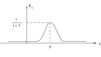
Figure 3: The “bounce” solution to Eq.(16) for fixed $\epsilon^{2}>1.$

The calculation of the integrals appearing in (15), as functions of $\epsilon^{2},$ is given in Appendix A. One obtains

$$J_{3}=-{3\over(\epsilon^{2}-1)^{2}}+{\epsilon^{2}+2\over(\epsilon^{2}-1)^{5/2}}tan^{-1}{\sqrt{\epsilon^{2}-1}}$$

$$J_{4}={4\epsilon^{2}+11\over 3(\epsilon^{2}-1)^{3}}-{3\epsilon^{2}+2\over(\epsilon^{2}-1)^{7/2}}tan^{-1}{\sqrt{\epsilon^{2}-1}}$$ (22)

$$\dot{J}_{2}={1\over 2}[J_{3}+(\epsilon^{2}-1)J_{4}].$$

The calculation of the prefactor ${\cal{N}}_{\varphi}$ is given in Appendix B. After isolating the zero mode, it involves the calculation of the determinant of a nontrivial non-local operator. We find

$${\cal{N}}_{\varphi}=\beta{\sqrt{n_{3}}}\tilde{\cal{N}}_{\varphi}$$

$$\tilde{\cal{N}}_{\varphi}={\sqrt{{8J_{4}\over\pi[6\dot{J}_{2}(J_{3}-J_{4})-2\epsilon^{2}J_{3}J_{4}]}}},$$ (23)

where $\beta$, coming from the zero mode, is the “volume” of the 1-dimensional Euclidean time, and the ${\sqrt{n_{3}}}$ factor in (23) comes from an identical factor appearing in the relation (14) between $\varphi_{c}$ and ${\tilde{\varphi}}_{c}.\ \tilde{\cal N}_{\varphi}$ is a function only of $\epsilon^{2}.$ One can show that it is an increasing function for $\epsilon^{2}>1.$ The limit

$$\tilde{\cal N}_{\varphi}^{2}\mathrel{{{}\atop{\longrightarrow}}\atop{{\epsilon^{2}\to 1}\atop{}}}15/\pi$$ (24)

shows that our solution is stable, that is it minimizes the effective action.

4 Asymptotic results for the large $n_{3},n_{4}$ perturbative coefficients and a numerical application

Because of the factorial growth of the perturbative coefficients in (10), which originates from the factor $exp(-S_{eff}[\varphi_{c}]),$ one can write the leading asymptotic series for Eq.(2) as

$$E(\alpha)-E(0)=\lim_{\beta\to\infty}\left(-{Z(\alpha)\over\beta}\right).$$ (25)

The error from this approximation appears only in the non-leading terms of the series [7]. Using Eqs.(10) and (23) one sees that the “volume” $\beta$ drops out and the ground state energy is

$$E(\alpha)={1\over 2}+\sum_{n_{3},n_{4}}\alpha^{n_{3}+n_{4}}E(n_{3},n_{4})$$ (26)

the coefficients being

$$E(n_{3},n_{4})={(-1)^{n_{4}+1}2{\sqrt{n_{3}}}{\tilde{\cal N}}_{\varphi}\ e^{-S_{eff}[\varphi_{c}]}\over(2n_{3})!n_{4}!2^{n_{4}}}.$$ (27)

Formulas (17), (19), (22), (23), (27) give complete results for the perturbative coefficients when $n_{3}$ and/or $n_{4}$ are large.

It is not difficult to find $E(n_{3},n_{4})$ numerically. For given $n_{3}$ and $n_{4}$ we first solve Eqs.(17) and (22) numerically to determine $\epsilon^{2}.$ Then we get $J_{3},J_{4},\dot{J}_{2}$ from (22), $S_{eff}[\varphi_{c}]$ from (19), ${\tilde{N}}_{\varphi}$ from (23) and finally $E(n_{3},n_{4})$ from (27). As an application we fix the order to be $n=n_{3}+n_{4}=10.$ We find the values $E(n_{3},n_{4})$ presented in Table 1. Because of the alternating sign of the series, delicate cancellations occur when we sum the terms and the result is

$$\sum_{n_{3}=0}^{10}E(n_{3},10-n_{3})=\ -2.019\times 10^{11}$$ (28)

which is 4 orders of magnitude smaller than the largest term. It is a well-known result[5], which we also derive using a different approach later in this paper, that

$$E(\alpha)=\sum_{n}E_{n}\alpha^{n}=\sum_{n}{-3^{n+1}n!\over\pi}\ \alpha^{n}$$ (29)

neglecting preasymptotics corrections which behave like $1/n$ compared to $E_{n}$[5, 10]. From (29) we obtain

Table 1: $E(n_{3},n_{4})$ for $n_{3}+n_{4}=n=10.$

$$E_{10}=-2.046\times 10^{11}$$ (30)

Comparing (28) and (30) we see that the error is 1.31%. As $n$ becomes larger, the error becomes smaller, and also both (27) and (29) are getting closer to the exact value. Recall that our approach is to use the steepest descent method around the saddle point $\varphi_{c}.$ We calculate only the Gaussian fluctuations. This will lead to equation (29) as we show in the following sections.

5 Borel transformation of the series

Neglecting the, unimportant for our purposes, zeroth order term $E(0)=1/2$ we can write (26) as

$$E(\alpha)={1\over\alpha}\int db\ e^{-{b\over\alpha}}\sum_{n_{3},n_{4}}{E(n_{3},n_{4})b^{n_{3}+n_{4}}\over(n_{3}+n_{4})!},$$ (31)

or

$$E(\alpha)={1\over\alpha}\int db\ e^{-{b\over\alpha}}\tilde{E}(b)$$ (32)

where the Borel transform $\tilde{E}(b)$ of the ground state energy is given by the series

$$\tilde{E}(b)=\sum_{n_{3},n_{4}}\ {b^{n_{3}+n_{4}}(-1)^{n_{4}+1}\ 2{\sqrt{n_{3}}}\ \tilde{\cal N}_{\varphi}e^{-S_{eff}[\varphi_{c}]}\over(2n_{3})!n_{4}!(n_{3}+n_{4})!2^{n_{4}}}.$$ (33)

In order to show that (27) is in exact agreement with (29) we shall show that $\tilde{E}(b),$ as given by (33), leads to a simple pole in the Borel plane with the residue demanded by (29). This requires transforming the $n_{4}$-sum in (33) into an integral and summing over $n_{3},$ tasks to which we now turn.

6 Analytical continuation in the complex $n_{4}$ plane and summation over the 3-vertices

The summand in (33) has a very complicated dependence on $\epsilon^{2}$ and the terms are of alternating sign in $n_{4}.$ The summation over $n_{4}$ cannot be done directly. We replace this summation by an integration over a contour in the complex $n_{4}$ plane in the following way. In general, let

$$\sigma=\sum_{n_{4}=0}^{\infty}(-1)^{n_{4}+1}\ f(n_{4})$$ (34)

then

$$\sigma={i\over 2}\int_{c^{\prime}}{dn_{4}f(n_{4})\over sin\pi n_{4}},$$ (35)

where the contour $c^{\prime}$ includes all non-negative integers and is shown in Fig.4. Now let $n_{4}=-\tilde{n}_{4},$ then

$$\sigma={i\over 2}\int_{c}{d\tilde{n}_{4}f(-\tilde{n}_{4})\over sin\pi\tilde{n}_{4}}$$ (36)

where $c$ is also shown in Fig.4. Using

$$\tilde{n}_{4}!(-\tilde{n}_{4})!={\pi\tilde{n}_{4}\over sin\pi\tilde{n}_{4}}$$ (37)

we finally get

$$\sigma={i\over 2\pi}\int_{c}{d\tilde{n}_{4}\over\tilde{n}_{4}}f(-\tilde{n}_{4})\tilde{n}_{4}!(-\tilde{n}_{4})!.$$ (38)

Figure 4: Contours of integration in the complex plane.

Therefore one can write $\tilde{E}(b)$ as

$$\tilde{E}(b)={i\over\pi}\sum_{n_{3}}\int_{c}d\tilde{n}_{4}{b^{n_{3}-\tilde{n}_{4}}2^{\tilde{n}_{4}}\tilde{n}_{4}!{\sqrt{n_{3}}}\tilde{\cal N}_{\varphi}e^{-S_{eff}[\varphi_{c}]}\over\tilde{n}_{4}(2n_{3})!(n_{3}-\tilde{n}_{4})!}.$$ (39)

Notice, as is shown in Fig.4, that one can extend the contour $c$ in (39) to include positive integers too, so long as $\tilde{n}_{4}<n_{3}.$ This will be important since, as we shall see, the dominant contribution will come from large and positive $\tilde{n}_{4}$ close to $n_{3}.$

In equation (39) one has to let $n_{4}\to-\tilde{n}_{4}$ in $S_{eff}[\varphi_{c}]$ and analytically continue the integrals $J_{3},J_{4},\dot{J}_{2}$ for complex $\epsilon^{2}$ as given in Appendix A. The variable $\epsilon^{2}$ clearly becomes

$$\epsilon^{2}=1-{\tilde{n}_{4}\over n_{3}}\ {J_{3}\over J_{4}}.$$ (40)

Using Stirling’s approximation for the factorials, (39) becomes

$$\tilde{E}(b)={i\over{\sqrt{4\pi^{3}}}}\sum_{n_{3}}\int_{c}d\tilde{n}_{4}\ {\tilde{\cal N}_{\varphi}e^{-n_{3}A}\over{\sqrt{\tilde{n}_{4}(n_{3}-\tilde{n}_{4})}}}$$ (41)

where A is a function of $\epsilon^{2}$ and  b  and is given by

$$A={2\dot{J}_{2}\over J_{3}}log{\dot{J}_{2}\over b}\ -\ {(1-\epsilon^{2})J_{4}\over J_{3}}\ log(1-\epsilon^{2}).$$ (42)

Since  A depends on $n_{3},\tilde{n}_{4}$ only through their ratio, we change variables from $n_{3}$ and $\tilde{n}_{4}$ to $n_{3}$ and $r$ where

$$\tilde{n}_{4}=n_{3}r$$ (43)

and hence

$$d\tilde{n}_{4}=n_{3}dr.$$ (44)

Then Eq.(41) becomes

$$\tilde{E}(b)={i\over{\sqrt{4\pi^{3}}}}\int{dr\tilde{\cal N}_{\varphi}\over{\sqrt{r(1-r)}}}\sum_{n_{3}=0}^{\infty}e^{-n_{3}A}.$$ (45)

The summation over the 3-vertices is now trivial leading to

$$\tilde{E}(b)={i\over{\sqrt{4\pi^{3}}}}\int{dr\tilde{\cal{N}}_{\varphi}\over{\sqrt{r(1-r)}}(1-e^{-A})}.$$ (46)

7 The singularity in the Borel plane

As is clear from (46) the singularity of $\tilde{E}(b)$ will come at a value of b where A vanishes. It is not too difficult to see that the important region of integration in equation (46) is for small $\epsilon^{2}.$ Defining

$$T=-log{\epsilon^{2}\over 4}$$ (47)

and using the expansions of Appendix A we have

$$\tilde{\cal N}_{\varphi}={\sqrt{6T\over\pi}}$$ (48)

$$r=1-{2\over 3T}$$ (49)

$$dr={2\over 3T^{2}}dT$$ (50)

and

$$A={2\over T}(\delta b-2e^{-T}),$$ (51)

where $\delta b={1/3}-b$ is small. Substitution of the above in (46) gives

$$\tilde{E}(b)={i\over 2\pi^{2}}\int{dT\over\delta b-2e^{-T}}.$$ (52)

Figure 5: The contour in the  z plane near the pole.

Defining $z=2\ e^{-T}$  and using  $dz=-zdT$ we get

$$\tilde{E}(b)={i\over 2\pi^{2}}\int{dz\over z(z-\delta b)}.$$ (53)

where the integration contour in (53) is shown in Fig.5, in the region where a pinch occurs. The integrand has a first-order pole at $\delta b$ and the residue is $1/\delta b.$ Thus we finally find

$$\tilde{E}(b)=-{1\over\pi}\ \ {1\over{1\over 3}-b}$$ (54)

which is the well-known result[5, 6, 8]. The Borel transform of the ground state energy has a 1st order pole at $b=1/3$ with residue $1/\pi.$ Using (54), Eq.(32) gives the leading asymptotic series in Eq.(29).

Finally we note that as $1/3-b$ becomes small the pinch in the z-integration in (53) at $z=0$ (or at $T=\infty$) corresponds to a pinch of the $r-$integration contour in (46) at $r=1$ as is evident from (49). This means that one can view the pole in $\tilde{E}(b)$ at $b=1/3$ as being determined by a particular “graph” having $n_{3}\approx-n_{4}=\tilde{n}_{4}$ large, that is a large but negative number of 4-vertices.

8 The $I-\bar{I}$ pair and comments

The classical solution (21) can also be expressed as

$$\varphi_{c}={\sqrt{{n\over\dot{J}_{2}}}}\ \ {1\over 1+\epsilon ch(t-\tau)}$$ (55)

where $n=n_{3}+n_{4}=n_{3}-\tilde{n_{4}}.$ Therefore $\varphi_{c}$ grows with the square root of the order in the perturbation series[7]. When $\epsilon^{2}$ is small, $\dot{J}_{2}$ is close to $1/3$ leading to

$$\varphi_{c}\approx{\sqrt{3n}}\ {1\over 1+\epsilon ch(t-\tau)}.$$ (56)

Now consider a “standard” approximate solution [5, 6, 8] to the equation of motion

$$-\ddot{\varphi}+\varphi=3{\sqrt{\alpha}}\ \varphi^{2}-2\alpha\varphi^{3}$$ (57)

corresponding to the Lagrangian given by (1)

$$\varphi={1\over{\sqrt{\alpha}}}\{{1\over e^{-(t-\tau+{\tilde{T}\over 2})}+1}\ +\ {1\over e^{t-\tau-{\tilde{T}\over 2}}+1}-1\}.$$ (58)

The instanton has its center at $\tau-\tilde{T}/2$ and the antiinstanton at $\tau+\tilde{T}/2,$ their separation being $\tilde{T}.$ When $\tilde{T}$ is large, (58) is an approximate solution to (57). It may be written in the form

$$\varphi={1\over{\sqrt{\alpha}}}{th{\tilde{T}\over 2}\over 1+(ch{\tilde{T}\over 2})^{-1}ch(t-\tau)},$$ (59)

and as $\tilde{T}\to\infty,$ or $\tilde{\epsilon}^{2}=4e^{-\tilde{T}}\to 0,$ one finds

$$\varphi\approx{1\over{\sqrt{\alpha}}}\ {1\over 1+\tilde{\epsilon}ch(t-\tau)}.$$ (60)

Figure 6: The $I-\bar{I}$ pair.

Comparing (56), (60) we see that our exact solution of $S_{eff}$ represents an $I-\bar{I}$ pair centered at $t=\tau$ and the separation is $T=-\log(\epsilon^{2}/4).$ This is shown in Fig.6. The small $\epsilon^{2}$ term in (16) is the difference between equations (16) and (57), but this is what allows us to have an exact $I-\bar{I}$ solution. Fig.7 shows the effective potential for fixed small $\epsilon^{2}.$ The conclusion is that the solution of the differential equation (16) which describes large order graphs is an $I-\bar{I}$ pair. This pair is a large fluctuation of the vacuum, but it has zero topological charge, and it emerges in a perturbative approach.

Figure 7: The effective potential for small $\epsilon^{2}.$ The dotted line represents the classical path.

It is also instructive to compare the coefficients ${\sqrt{3n}}$ and $1/{\sqrt{\alpha}}$ in (56), (60). These coefficients become equal when

$$3\alpha n=1.$$ (61)

To interpret this we differentiate $E_{n}$ of Eq.(29) to see when the asymptotic series starts to diverge. One finds that ${dE_{n}\over dn}=0$ exactly when (61) is satisfied so that the solution, (56), determining the large orders of the perturbation theory agrees with the $I-\bar{I}$ approximate solution of the original Lagrangian just when the perturbation series starts to diverge.

Finally, we make a couple of comments. As mentioned earlier the value of the effective action does not depend on the position $\tau$ of the center of the $I-\bar{I}$ pair. As can be seen from Appendix B, the existence of this “collective coordinate” results in a factor

$$\Delta={\sqrt{{2n_{3}\dot{J}_{2}\over J_{3}}}}={\sqrt{n}}.$$ (62)

This is equivalent to the statement that in a general interacting theory with coupling $\alpha,$ each collective coordinate, which comes from a symmetry, results in a factor $1/{\sqrt{\alpha}}.$ One should also comment on the quasizero mode[11] which normally appears as a fluctuation of the $I-\bar{I}$ separation. In Appendix B we calculate the determinantal ratio $det^{\prime}(K+U)/detK_{0}$ which is $(18T^{2})^{-1}$ for large $T.$ It looks as if there exists a small eigenvalue with eigenfunction, say, $\eta_{1}.$ However, the fluctuation of the action along $\eta_{1}$ is large. From the scaling relation (14) one has

$$\eta_{1}\sim{\sqrt{{n_{3}\over J_{3}}}}\sim{\sqrt{{n_{3}\over T}}}.$$ (63)

Therefore, there is an additional overall factor of $n_{3}/T$ coming into the effective action (see (B2) and (B3)) leading to

$$\Delta S_{eff}\sim\lambda_{1}\eta_{1}^{2}\sim n_{3}/T^{3}$$ (64)

from the eigenmode corresponding to $\eta_{1}.$ From (45), (46), and (51) we see that the important region of $n_{3}$ is

$$n_{3}\sim{1\over A}\sim{T\over\epsilon^{2}}.$$ (65)

Thus (64) becomes

$$\Delta S_{eff}\sim{1\over\epsilon^{2}T^{2}}\mathrel{{{}\atop{\longrightarrow}}\atop{\epsilon^{2}\to 0}}\infty.$$

APPENDIX A Here we calculate the integrals $J_{3},J_{4}$ and $\dot{J}_{2}$ as functions of $\epsilon^{2},$ first for $\epsilon^{2}>1.$ We start from the integral

$$J(a)=\int_{-\infty}^{\infty}{dt\over a+\epsilon cht}={2\over{\sqrt{\epsilon^{2}-a^{2}}}}tan^{-1}{\sqrt{{\epsilon^{2}\over a^{2}}-1}}$$

for $a<\epsilon.$ Differentiating with respect to  $a\$ and setting $a=1$ we get $J_{3},J_{4}$ from

$$J_{n+1}=\int_{-\infty}^{\infty}{dt\over(a+\epsilon cht)^{n+1}}={(-1)^{n}\over n!}\ {d^{n}J(a)\over da^{n}}\bigg{|}_{a=1}.$$

Thus

$$J_{3}=-\ {3\over(\epsilon^{2}-1)^{2}}\ +\ {\epsilon^{2}+2\over(\epsilon^{2}-1)^{5/2}}\ tan^{-1}{\sqrt{\epsilon^{2}-1}},$$

and

$$J_{4}={4\epsilon^{2}+11\over 3(\epsilon^{2}-1)^{3}}\ -\ {3\epsilon^{2}+2\over(\epsilon^{2}-1)^{7/2}}tan^{-1}{\sqrt{\epsilon^{2}-1}}.$$

One can obtain $\dot{J}_{2}$ by using the differential equation (16):

$$-\ddot{\tilde{\varphi_{c}}}+\tilde{\varphi_{c}}=3\tilde{\varphi_{c}}^{2}+2(\epsilon^{2}-1)\tilde{\varphi_{c}}^{3}.$$

Multiplying (A5) by $\dot{\tilde{\varphi_{c}}}$ and integrating one obtains

$$\dot{J}_{2}-J_{2}=-2J_{3}-(\epsilon^{2}-1)J_{4}.$$

Multiplying (A5) by $\tilde{\varphi_{c}}$ and integrating gives

$$\dot{J}_{2}+J_{2}=3J_{3}+2(\epsilon^{2}-1)J_{4}.$$

Equations (A6) and (A7) give

$$\dot{J}_{2}={1\over 2}[J_{3}+(\epsilon^{2}-1)J_{4}].$$

One may use the above equations for complex $\epsilon^{2}.$ Since we need the integrals for small and complex $\epsilon^{2}$ we write them in the more convenient form

$$J_{3}=-{3\over(1-\epsilon^{2})^{2}}+{2+\epsilon^{2}\over(1-\epsilon^{2})^{5/2}}th^{-1}{\sqrt{1-\epsilon^{2}}}$$

$$J_{4}=-{11+4\epsilon^{2}\over 3(1-\epsilon^{2})^{3}}+{2+3\epsilon^{2}\over(1-\epsilon^{2})^{7/2}}th^{-1}{\sqrt{1-\epsilon^{2}}},$$

where $\dot{J}_{2}$ is still given by (A8). The expansions to order $\epsilon^{2},$ for small $\epsilon^{2}$ or equivalently large $T=-log(\epsilon^{2}/4),$ are:

$$J_{3}=T-3+(12T-26)\ {\epsilon^{2}\over 4}$$

$$J_{4}=T-{11\over 3}+(20T-{154\over 3})\ {\epsilon^{2}\over 4}$$

$$\dot{J}_{2}={1\over 3}-(2T-{16\over 3})\ {\epsilon^{2}\over 4}$$

$${\tilde{n}_{4}\over n_{3}}=1-{2\over 3(T-3)}+{4[T(3T-11)+11]\over 3(T-3)^{2}}\ {\epsilon^{2}\over 4}$$

where we have used (40) to derive (A14).

Appendix B Here we calculate the prefactor ${\cal N}_{\varphi}.$ The effective action is given by (9). Its second derivate evaluated at the saddle point $\varphi_{c}$ is given by

$${\delta^{2}S_{eff}\over\delta\varphi(t^{\prime})\delta\varphi(t)}\bigg{|}_{\varphi_{c}}=\{{-d^{2}\over dt^{2}}\ +1-6\tilde{\varphi}_{c}(t-\tau)-6(\epsilon^{2}-1)\tilde{\varphi}_{c}^{2}(t-\tau)\}\delta(t-t^{\prime})$$

$$+{9\over J_{3}}\tilde{\varphi}_{c}^{2}(t-\tau)\tilde{\varphi}_{c}^{2}(t^{\prime}-\tau)+{8(\epsilon^{2}-1)\over J_{4}}\tilde{\varphi}_{c}^{3}(t-\tau)\tilde{\varphi}_{c}^{3}(t^{\prime}-\tau).$$

Let $\eta(t)$ be the small fluctuation around $\varphi_{c}(t-\tau).$ Then the small fluctuation action is

$$\Delta S_{eff}={1\over 2}\int dtdt^{\prime}{\delta^{2}S_{eff}\over\delta\varphi(t^{\prime})\delta\varphi(t)}\bigg{|}_{\varphi_{c}}\eta(t)\eta(t^{\prime}).$$

Substituting (B1) into (B2) we can write $\Delta S_{eff}$ in a convenient bracket notation[7] as

$$\Delta S_{eff}={1\over 2}<\eta|(K+U)_{\tau}|\eta>$$

with

$$K=K_{0}-6\tilde{\varphi}_{c}-6(\epsilon^{2}-1)\tilde{\varphi}_{c}^{2}$$

$$U={9\over J_{3}}|\tilde{\varphi}_{c}^{2}><\tilde{\varphi}_{c}^{2}|+{8(\epsilon^{2}-1)\over J_{4}}|\tilde{\varphi}_{c}^{3}><\tilde{\varphi}_{c}^{3}|.$$

The index $\tau$ means that the argument of $\tilde{\varphi}_{c}$ is $t-\tau.$

Thus the prefactor is

$${\cal{N}}_{\varphi}={\int\ D\eta\ exp\{-{1\over 2}<\eta|(K+U)_{\tau}|\eta>\}\over\int\ D\eta\ exp\{-{1\over 2}<\eta|K_{0}|\eta>\}}.$$

The nonlocal operator $(K+U)_{\tau}$ has a zero mode given by $\dot{\tilde{\varphi}}_{c}(t-\tau).$ First notice that

$$U|\dot{\tilde{\varphi}}_{c}>=0$$

since $<\tilde{\varphi}_{c}^{2}|\dot{\tilde{\varphi}}_{c}>\ =\ <\tilde{\varphi}_{c}^{3}|\dot{\tilde{\varphi}}_{c}>=0$ because $\tilde{\varphi}_{c}$ is even while $\dot{\tilde{\varphi}}_{c}$ is odd. Also

$$K\dot{\tilde{\varphi}}_{c}=K_{0}\dot{\tilde{\varphi}}_{c}-6\tilde{\varphi}_{c}\dot{\tilde{\varphi}}_{c}-6(\epsilon^{2}-1)\tilde{\varphi}_{c}^{2}\dot{\tilde{\varphi}}_{c}$$

$$={d\over dt}(3\tilde{\varphi}_{c}^{2}+2(\epsilon^{2}-1)\tilde{\varphi}_{c}^{3})-6\tilde{\varphi}_{c}\dot{\tilde{\varphi}}_{c}-6(\epsilon^{2}-1)\tilde{\varphi_{c}}^{2}\dot{\tilde{\varphi}}_{c}$$

implies

$$K\dot{\tilde{\varphi}}_{c}=0.$$

Therefore

$$(K+U)_{\tau}|\dot{\tilde{\varphi}}_{c}(t-\tau)>=0.$$

Since $<\dot{\tilde{\varphi}}_{c}|\dot{\tilde{\varphi}_{c}}>=\dot{J}_{2}$ we define the zero frequency normalized eigenfunction by

$$\eta_{0}(t-\tau)={\dot{\tilde{\varphi}}_{c}(t-\tau)\over{\sqrt{\dot{J}_{2}}}}.$$

Now use the Fadeev-Popov trick to change the zero eigenvalue into a collective coordinate integration

$$1=\int d\tau\delta(<\eta(t)|\eta_{0}(t-\tau)>)\Delta$$

where

$$\Delta={d\over d\tau}<\eta(t)|\eta_{0}(t-\tau)>.$$

Equation (B12) leads to

$$\Delta=<\dot{\varphi}(t)|\eta_{0}(t-\tau)>.$$

In the sense of the steepest descent method $\dot{\varphi}(t)$ may be approximated by $\dot{\varphi}_{c}(t-\tau)$ so that

$$\Delta=<\dot{\varphi}_{c}(t-\tau)|\eta_{0}(t-\tau)>$$

giving finally

$$\Delta={\sqrt{{2n_{3}\dot{J}_{2}\over J_{3}}}}.$$

The identity (B11) is inserted in the functional integral expression (B6) for ${\cal N}_{\varphi}$ giving

$${\cal N}_{\varphi}={\Delta\int d\tau\int D\eta\delta(<\eta|\eta_{0}(t-\tau)>)exp\{-{1\over 2}<\eta|(K+U)_{\tau}|\eta>\}\over\int D\eta\ exp\{-{1\over 2}<\eta|\ K_{0}|\eta>\}}.$$

In the numerator of (B16) the functional integral is independent of $\tau,$ so we can choose, say, $\tau=0.$ The integration over $\tau$ is trivial and gives the one-dimensional volume of time $\beta.$ Thus

$${\cal{N}}_{\varphi}={\beta\Delta\over{\sqrt{2\pi}}}{\sqrt{{detK_{0}\over det^{\prime}(K+U)}}}$$

where the prime means that the zero eigenvalue is omitted because of the $\delta-$function in (B16).

Now we turn to the nonlocal part U. In general

$$det(K+\sum_{\alpha=1}^{N}|\alpha><\alpha|)=detK\cdot det(1+\sum_{\alpha=1}^{N}K^{-1}|\alpha><\alpha|)$$

where $K^{-1}$ is well-defined and is linear. The second determinant can be shown to obey

$$det(1+\sum_{\alpha=1}^{N}K^{-1}|\alpha><\alpha|)=det(1+\hat{K}^{-1})$$

where on the right-hand side of (B19) $\hat{K}^{-1}$ is a $N\times N$ matrix with elements

$$\hat{K}_{\alpha\alpha^{\prime}}^{-1}=<\alpha|K^{-1}|\alpha^{\prime}>.$$

In our case $K^{-1}$ is well-defined because we consider the primed determinant. The operation of $K^{-1}$ on $|\tilde{\varphi}_{c}^{2}>,|\tilde{\varphi}_{c}^{3}>$ is also defined because these states are orthogonal to the zero mode. Thus

$$det^{\prime}(K+U)=det^{\prime}K\cdot det(1+\hat{K}^{-1})$$

$$det(1+\hat{K}^{-1})=(1+{9\over J_{3}}\hat{K}_{22}^{-1})(1+{8(\epsilon^{2}-1)\over J_{4}}\hat{K}_{33}^{-1})-{72(\epsilon^{2}-1)\over J_{3}J_{4}}(\hat{K}_{23}^{-1})^{2}.$$

It is not difficult to find the three matrix elements. Start from the operation of $K$ on $\tilde{\varphi}_{c}:$

$$K\tilde{\varphi}_{c}=-3\tilde{\varphi}_{c}^{2}-4(\epsilon^{2}-1)\tilde{\varphi}_{c}^{3}$$

$$\tilde{\varphi}_{c}=-3K^{-1}\tilde{\varphi}_{c}^{2}-4(\epsilon^{2}-1)K^{-1}\tilde{\varphi}_{c}^{3}.$$

Multiplying (B23) by $\tilde{\varphi}_{c}^{2}$ and $\tilde{\varphi}_{c}^{3}$ in turn and integrating gives

$$J_{3}=-3\hat{K}_{22}^{-1}-4(\epsilon^{2}-1)\hat{K}_{23}^{-1}$$

and

$$J_{4}=-3\hat{K}_{23}^{-1}-4(\epsilon^{2}-1)\hat{K}_{33}^{-1}.$$

A third equation may be obtained from the operation of $K$ on $\tilde{\varphi}_{c}^{2}$ in a similar way:

$$K\tilde{\varphi}_{c}^{2}=-3\tilde{\varphi}_{c}^{2}+4\tilde{\varphi}_{c}^{3}$$

$$\tilde{\varphi}_{c}^{-}3K^{-1}\tilde{\varphi}_{c}^{2}+4K^{-1}\tilde{\varphi}_{c}^{3}$$

$$J_{4}=-3\hat{K}_{22}^{-1}+4\hat{K}_{23}^{-1}.$$

Solving (B24), (B25), (B26) we find the matrix elements and (B22) gives

$$det(1+\hat{K}^{-1})=2-{6\dot{J}_{2}(J_{3}-J_{4})\over\epsilon^{2}J_{3}J_{4}}.$$

Finally, we need to calculate the ratio of determinants $det^{\prime}K/detK_{0}.$ We consider a finite sized “volume” $\beta.$ Then $K$ has no zero eigenvalue, since translation symmetry is lost, but there is a small eigenvalue $\lambda_{0}$ which goes to zero as $\beta\to\infty.$ The determinantal ratio can be obtained just from he knowledge of the classical solution. Following references[12, 13] one writes

$${det^{\prime}K\over detK_{0}}\ =\lim_{\beta\to\infty}\ {\psi(\beta/2)\over\lambda_{0}\psi^{(0)}(\beta/2)}$$

where $\psi(t),\psi^{(0)}(t)$ are zero eigenvalue solutions of $K,K_{0}$ respectively, which do not vanish at $t=\beta/2,$ but satisfy the boundary conditions

$$\psi(-\beta/2)=0,\ \ \ \ \ \ \ \ \ \dot{\psi}(-\beta/2)=1,$$

with analogous boundary conditions for $\psi^{(0)}.$ It is trivial to find $\psi^{(0)}(\beta/2)$ for the free theory:

$$\psi^{(0)}(t)=sh(t+\beta/2)$$

$$\psi^{(0)}(\beta/2)=sh\beta$$

$$\psi^{(0)}(\beta/2)\mathrel{}{{{}\atop{\longrightarrow}}\atop{\beta\to\infty}}e^{\beta}/2.$$

Now we need to find $\psi(t).$ We already know one solution $\dot{\tilde{\varphi}}_{c}$ satisfying $K\dot{\tilde{\varphi}}_{c}=0.$ For convenience we normalize it to be $-{\epsilon\over 2}\dot{\tilde{\varphi}}_{c}$ and call it $\psi_{1}.$ We need only the asymptotic behavior

$$\psi_{1}\mathrel{}{{{}\atop{\simeq}}\atop{{t\to\pm\infty}}}\pm e^{-|t|}.$$

A second independent solution is

$$\psi_{2}\sim\psi_{1}(t)\int^{t}{dt^{\prime}\over\psi_{1}^{2}(t^{\prime})},$$

which leads to

$$\psi_{2}\mathrel{}{{{}\atop{\simeq}}\atop{t\to\pm\infty}}e^{|t|}.$$

As expected $\psi_{2}$ has the opposite exponential behavior from $\psi_{1},$ and $\psi_{2}$ is even while $\psi_{1}$ is odd. One can write the linear combination of $\psi_{1},\psi_{2}$ which satisfies (B29) as

$$\psi(t)={1\over 2}\{\psi_{1}(-\beta/2)\psi_{2}(t)-\psi_{2}(-\beta/2)\psi_{1}(t)\}$$

and its value at $t=\beta/2\ {\rm as}\ \beta\to\infty$ is

$$\psi(\beta/2)\mathrel{{{}\atop{\longrightarrow}}\atop{\beta\to\infty}}-1.$$

It remains to get the small eigenvalues $\lambda_{0}.$ To first order in perturbation theory the solution $\psi_{\beta}(t)$ that vanishes at $t=\pm\beta/2$ is

$$\psi_{\beta}(t)=\psi(t)+{\lambda_{0}\over 2}\int_{-\beta/2}^{t}dt^{\prime}\psi(t^{\prime})[\psi_{1}(t)\psi_{2}(t^{\prime})-\psi_{2}(t)\psi_{1}(t^{\prime})].$$

It is obvious that $\psi_{\beta}(-\beta/2)=0.$ Requiring $\psi_{\beta}(\beta/2)=0$ gives $\lambda_{0}$ as

$$\lambda_{0}=2[\psi_{1}(\beta/2)<\psi|\psi_{2}>-\psi_{2}(\beta/2)<\psi|\psi_{1}>]^{-1}.$$

Substituting $\psi$ from (B34) in (B37) and using $<\psi_{1}|\psi_{2}>=0$ gives

$$\lambda_{0}=4[-e^{-\beta}<\psi_{2}|\psi_{2}>+e^{\beta}<\psi_{1}|\psi_{1}>]^{-1}.$$

The dominant term in (B38) is the second one which diverges while the first one remains finite for $\beta\to\infty.$ We finally obtain

$$\lambda_{0}={16e^{-\beta}\over\epsilon^{2}\dot{J}_{2}}$$

which vanishes when $\beta\to\infty$ as claimed. Hence the determinantal ratio from (B28), (B30), (B35), (B39) is

$${det^{\prime}K\over detK_{0}}\ =\ -{\epsilon^{2}\dot{J}_{2}\over 8}.$$

The minus sign is not surprising since $K$ has a negative eigenvalue. Recall that the zero mode is odd with one node, therefore there should be an even mode with no nodes and a smaller, thus negative, eigenvalue. This minus sign causes no problem in the stability of the solution since $det(1+\hat{K}^{-1})$ is negative too leaving the saddle point $\varphi_{c}$ a minimum for the action[7]. Putting everything together from equations (B15), (B17), (B21), (B27) and (B40) the prefactor as a function of $n_{3}$ and $\epsilon^{2}$ is

$${\cal{N}}_{\varphi}=\beta{\sqrt{n_{3}}}\ \tilde{\cal N}_{\varphi}$$

$$\tilde{\cal N}_{\varphi}={\sqrt{{8J_{4}\over\pi[6\dot{J}_{2}(J_{3}-J_{4})-2\epsilon^{2}J_{3}J_{4}]}}}.$$

References

• [1] G. ’t Hooft, in: The why’s of subnuclear physics (Erice, 1977), ed. A. Zichichi.
• [2] For a review of renormalons see M. Beneke, Phys.Rep.317 (1999) 1.
• [3] L.N. Lipatov, Zh. Eksp.Teor.Fiz 72 (1977) 411.
• [4] G. Parisi, Phys. Lett. B68 (1977) 361.
• [5] E. Brezin, G. Parisi, and J. Zinn-Justin, Phys. Rev. D16 (1977) 408.
• [6] J. Zinn-Justin in Recent Advances in Field Theory and Statistical Mechanics, J.-B. Zuber and R. Stora, eds. Elsevier (1984).
• [7] C. Itzykson and J.B. Zuber, Quantum Field Theory (1980) 467.
• [8] E.B. Bogomolny, Phys. Lett.B91 (1980), 431.
• [9] I.I. Balitsky, Phys. Lett. B273 (1991), 282.
• [10] S.V. Faleev and P.G. Silvestrov, Phys. Lett. A197 (1995) 372.
• [11] I.I. Balitsky and A.V. Yung, Phys. Lett.B168 (1986) 113.
• [12] S. Coleman, Aspects of Symmetry (1985) 340.
• [13] H. Kleinert, Path Integrals in Quantum Mechanics, Statistics and Polymer Physics (1995) 714.