TTP00-16

hep-ph/0008262

Four Pion Final States with Tagged Photons
at Electron Positron Colliders

H. Czyż ^a , J.H. Kühn^b

• Institute of Physics, University of Silesia, ul. Uniwersytecka 4, PL-40007 Katowice, Poland

• Institut für Theoretische Teilchenphysik, Universität Karlsruhe, D-76128 Karlsruhe, Germany

e-mail: czyz@us.edu.pl
             johann.kuehn@physik.uni-karlsruhe.de

A Monte Carlo generator has been constructed to simulate the reaction $e^{+}e^{-}\to\gamma+4\pi$, where the photon is assumed to be observed in the detector. Only initial state radiation is considered. Additional collinear photon radiation has been incorporated with the technique of structure functions. Predictions are presented for cms energies of 1GeV, 3GeV and 10GeV, corresponding to the energies of DA$\Phi$NE, BEBC and of $B$-meson factories. The event rates are sufficiently high to allow for a precise measurement of $R(Q^{2})$ in the region of $Q$ between approximately 1GeV and 2.5GeV. For the construction of the program we employ isospin relations between the amplitudes governing $\tau$ decays into four pions and electron positron annihilation into four pions. Estimates of the kinematic breaking of these isospin relations as a consequence of the $\pi^{-}$ – $\pi^{0}$ mass difference are given.

1 Introduction.

The precise determination of the cross section for electron positron annihilation into hadrons over a large energy range is one of the important tasks of current particle physics. The results are relevant for the analysis of electroweak precision measurements which are affected by the running of the electromagnetic coupling from the Thompson limit up to $M_{Z}$. Also the interpretation of the anomalous magnetic moment of the muon depends critically on these data. Last not least the measurement of the energy dependence of R(s) is one of the gold plated tests of QCD and allows for a precise determination of the strong coupling constant.

Depending on the energy region different techniques for the measurement of $R(s)$ have been applied up to date. At low energies, say from the two pion threshold up to roughly two GeV, exclusive channels are collected separately, for higher energies inclusive measurements start to become dominant. For energies below $m_{\tau}$ isospin invariance and CVC have traditionally been used to predict $\tau$ decays from electron positron annihilation [1, 2, 3, 4]. Clearly this strategy can be inverted [5] pending irreducible uncertainties from isospin violation and radiative corrections [6]. At high energies a multitude of final states is present and only inclusive measurements have been performed.

To cover a large range of energies, results from many different experiments and colliders have to be combined, and energy scans have to be performed to obtain the full energy dependence. An attractive alternative is provided by the upcoming $\Phi-$ and $B-$ meson factories which operate at large luminosities, albeit at fixed energies. Events with radiated tagged photons give access to a measurement of $R$ over the full range of energies, from threshold up to the CMS energy of the collider. For events with tagged photons the invariant mass of the recoiling hadronic system is fixed by the photon energy which provides an important kinematic constraint. The usage of photons observed at extremely small angle with respect to the beam has been investigated in [7, 8]. In this case final state radiation as background is practically irrelevant. However, in practice photon detectors do not cover this region. At large angles a careful study of initial versus final state radiation has to be performed.

To arrive at reliable predictions including angular and energy cutoffs as employed by realistic experiments, a Monte Carlo generator is indispensable. For hadronic states with invariant masses below two or even three GeV it is desirable to simulate the individual exclusive channels with two, three up to six mesons i.e. pions, kaons, etas etc. which requires a fairly detailed parametrization of the various form factors.

In principle initial and final state radiation would be required for the complete simulation. Such a program has been constructed for the two pion case [9]. There it is demonstrated that suitably chosen configurations, namely those with hard photons at small angles relative to the beam and well separated from the pions, are dominated by initial state radiation. In fact, this separation is possible [10] even when operating the $\phi$ factory DA$\Phi$NE on top of the $\phi$ resonance where direct radiative $\phi$ decays cannot be ignored.

In the present paper we continue this project with the construction of a generator for the radiative production of the four pion final state, including the $\omega(\to 3\pi)\pi$ channel. This mode contributes a large fraction of the rate with invariant masses between one and two GeV. The energy region between 1.5 GeV and 2.5 GeV is difficult to access directly with current electron positron colliders. At the same time the experimental uncertainties are relatively large. This motivates the special effort devoted to this range.

The Monte Carlo program discussed in the present paper is specifically devoted to cms energies up to approximately 10 GeV. It is constructed in a modular form such that the parametrization of the hadronic matrix element can easily be replaced by a more elaborate version. Different final states with three, four or five pions or kaons can be included. The present parametrization of the hadronic matrix element follows closely the form suggested in [11], correcting only some minor deficiencies. The four pion amplitude is assumed to be dominated by $\rho\prime\to\pi a_{1}$ plus a direct coupling $\rho\prime\to\rho\pi\pi$ and exhibits the proper behavior in the chiral limit.

The plan of this paper is as follows: In the next section the formalism for the decomposition of the differential cross section into a leptonic and a hadronic tensor is presented. Results for partially integrated distributions are recalled which can easily be used to arrive at simple estimates for the rates. In section 3 isospin relations are derived between the amplitudes for four pion production from a virtual photon and those accessible in $\tau$ decay. The relations between these four matrix elements contain the well known identities between the corresponding rates and provide in addition important constraints on the differential distributions. In section 4 the influence of the $\pi^{0}-\pi^{\pm}$ mass difference on the relations obtained in section 3 is discussed. The ingredients of the ansatz for the hadronic amplitude together with a comparison between the model prediction and the data for a variety of distributions are presented in section 5, the complete description of the hadronic amplitude with all the model parameters is collected in the appendix. A description of the Monte Carlo generator is given in section 6, together with a few characteristic distributions. In particular we investigate the influence of angular cuts and the addition of collinear radiation. Section 7 contains a brief summary and the conclusions.

2 The radiative return.

Hard photons observed at small angles relative to the electron or positron beam and at the same time well separated from charged particles in the final state can be used to reduce the effective center of mass energy at electron positron colliders. Performing a detailed analysis of the angular and energy distributions for the $\gamma\pi^{+}\pi^{-}$ final state it has been shown that initial and final state radiation can be reasonably well separated [9, 10]. For the four pion case we therefore restrict the discussion to initial state radiation only. The matrix element for the production of an arbitrary hadronic final state corresponding to the diagrams Fig.1 are given by

$${\cal M}=i\ e^{3}\ \bar{v}\left(p_{+}\right)\left[\gamma^{\nu}\frac{1}{p_{-}{\kern-12.0pt}/-k{\kern-5.0pt}/-m}\epsilon^{*}{\kern-10.0pt}/\left(k\right)+\epsilon^{*}{\kern-10.0pt}/\left(k\right)\frac{1}{k{\kern-5.0pt}/-p_{+}{\kern-12.0pt}/-m}\gamma^{\nu}\right]\frac{1}{Q^{2}}\ J^{em}_{\nu}\ .$$ (1)

Figure 1: Diagrams contributing to the process $e^{+}e^{-}\to\gamma+hadrons$ (only initial state radiation included).

The matrix element of the hadronic current

$$J^{em}_{\nu}\ \equiv\ J^{em}_{\nu}\left(q_{1},...,q_{n}\right)\ \equiv\ <h(q_{1}),...,h(q_{n})|J^{em}_{\nu}\left(0\right)|0>$$ (2)

has to be parameterized by form factors to be discussed below. For the two pion case the current

$$J_{\nu}^{em,2\pi}=\left(q_{\nu}^{+}-q_{\nu}^{-}\right)F_{2\pi}\left(Q^{2}\right)$$ (3)

is determined by only one function, the pion form factor $F_{2\pi}$.

For the three pion case the matrix element of the electromagnetic current is restricted by current conservation and negative parity to the form

$$J_{\nu}^{em,3\pi}=\epsilon_{\nu\alpha\beta\gamma}\ q_{+}^{\alpha}q_{-}^{\beta}q_{0}^{\gamma}\ F_{3\pi}\left(q_{+},q_{-},q_{0}\right)$$ (4)

and $F_{3\pi}$ is dominated by the $\omega$ resonance. The matrix element for the four pion case will be discussed in sections 3 and 4.

The differential rate can be cast into a product of a leptonic and a hadronic tensor and a corresponding separation of the phase space

$$d\sigma=\frac{1}{8s}\ L_{\mu\nu}H^{\mu\nu}\ d\Phi_{2}(p_{+}+p_{-};Q,k)\ d\bar{\Phi}_{n}(Q;q_{1},\dots,q_{n})\ \frac{dQ^{2}}{2\pi}\ ,$$ (5)

where $d\bar{\Phi}_{n}(Q;q_{1},\dots,q_{n})$ denotes the $n$ body phase space with all statistical factors included.

The leptonic tensor $L_{\mu\nu}$ is process independent, the modeling of hadronic physics enters the tensor $H_{\mu\nu}=J^{em}_{\mu}(J^{em}_{\nu})^{*}$ only. The leptonic tensor is symmetric, and hence it is only the real symmetric part of $H_{\mu\nu}$ which enters. It has the following form

$$L^{\mu\nu}=\frac{-4}{(kp_{-})(kp_{+})}\left[\ g^{\mu\nu}\ \left(p_{-}p_{+}+\frac{(kp_{+})^{2}+(kp_{-})^{2}}{Q^{2}}\right)+\ \ p_{+}^{\mu}p_{+}^{\nu}+p_{-}^{\mu}p_{-}^{\nu}\ \right]\frac{1}{Q^{2}}\ .$$ (6)

The collinear and soft photon singularities proportional to $1/(1\pm\cos\theta_{\gamma})$ and $1/E_{\gamma}$ are evident from these expressions, as well as the $1/Q^{2}$ enhancement for small $Q^{2}$. Integrating the hadronic tensor $H_{\mu\nu}$ over the hadronic phase space one gets

$$\int\ J^{em}_{\mu}(J^{em}_{\nu})^{*}\ \ d\bar{\Phi}_{n}(Q;q_{1},\dots,q_{n})=\frac{1}{6\pi}\left(Q_{\mu}Q_{\nu}-g_{\mu\nu}Q^{2}\right)\ R(Q^{2})$$ (7)

where $R(Q^{2})$ is $\sigma(e^{+}e^{-}\rightarrow hadrons)/\sigma_{point}$.

$$\begin{array}[]{||c||c||c||c|c|c||}\hline\cr&&&\vrule\lx@intercol\hfil{\rm Event~{}rates}\hfil\lx@intercol\vrule\lx@intercol\\ \hline\cr{\rm Collider}&\sqrt{s}&{\rm Integrated~{}luminosity},{\rm fb}^{-1}&\theta_{\rm min}=5^{\circ}&\theta_{\rm min}=7^{\circ}&\theta_{\rm min}=10^{\circ}\\ \hline\cr\hline\cr{\rm DA}\Phi{\rm NE}&1.02&1&13\cdot 10^{6}&12\cdot 10^{6}&10\cdot 10^{6}\\ \hline\cr\hline\cr B-{\rm factory}&10.6&100&4\cdot 10^{6}&3.5\cdot 10^{6}&3\cdot 10^{6}\\ \hline\cr\hline\cr{B-\rm factory}&10.6&100&2.7\cdot 10^{6}&2.3\cdot 10^{6}&2.0\cdot 10^{6}\\ \hline\cr\end{array}$$

Table 1: Estimated number of radiative events $e^{+}e^{-}\to\ hadrons\ +\ \gamma$ for different center of mass energies from Eq.(8). In the first two rows by $hadrons$ we mean $\pi^{+}\pi^{-}$ and the minimal photon energy is $0.1$ GeV. The third row is obtained for a continuum contribution in the region $2\ {\rm GeV}<\sqrt{Q^{2}}<3.7\ {\rm GeV}$ assuming a constant $R=2.4$.

The additional integration over the photon angles (the azimuthal angle is integrated over the full range and the polar angle within $\theta_{min}<\theta<\pi-\theta_{min}$ ) leads to the differential distribution

$$Q^{2}\frac{{\rm d}\sigma}{{\rm d}Q^{2}}=\frac{4\alpha^{3}}{3s}R(Q^{2})\left\{\frac{(s^{2}+Q^{4})}{s(s-Q^{2})}\log\frac{1+\cos\theta_{\rm min}}{1-\cos\theta_{\rm min}}-\frac{(s-Q^{2})}{s}\cos\theta_{\rm min}\right\}\ ,$$ (8)

which can be used to calculate the event rate observed for realistic photon energy and angular cuts (see Tab.1).

3 Isospin relations.

The emphasis of this paper is towards hadronic final states consisting of four pions and a photon. Before entering a discussion of a model dependent parametrization of the form factors (see section 5) we recall the constraints from isospin invariance. They relate the amplitudes of the $e^{+}e^{-}\to 2\pi^{+}2\pi^{-}$ and $e^{+}e^{-}\to\pi^{+}\pi^{-}2\pi^{0}$ processes and those for $\tau$ decays into $\pi^{-}3\pi^{0}$ and $\pi^{+}2\pi^{-}\pi^{0}$. The amplitude of the $\tau$ decay into an arbitrary number of hadrons plus a neutrino is given by

$${\cal M}_{\tau}=\ \ \frac{G_{F}}{\sqrt{2}}\ \cos\theta_{c}\ \ \bar{v}\left(p_{\nu}\right)\gamma^{\alpha}\left(1-\gamma_{5}\right)u\left(p_{\tau}\right)\ \ J_{\alpha}^{-}\ ,$$ (9)

with

$$J^{-}_{\alpha}\ \equiv\ J^{-}_{\alpha}\left(q_{1},...,q_{n}\right)\ \equiv\ <h(q_{1}),...,h(q_{n})|J^{-}_{\alpha}\left(0\right)|0>$$

$${\kern-30.0pt}{\rm and}\ \ \ \ \ J^{-}_{\alpha}(0)=\bar{d}\ \gamma_{\alpha}\ u\ \ \ .$$ (10)

We use the same letter $J$ for the operator and its matrix element and restrict our considerations to the Cabbibo allowed vector part of the hadronic current.

It leads to the differential distribution

$$\frac{d\Gamma}{dQ^{2}}=2\ \Gamma_{e}\frac{\cos^{2}\theta_{c}}{m_{\tau}^{2}}\left(1-\frac{Q^{2}}{m_{\tau}^{2}}\right)^{2}\left(1+2\frac{Q^{2}}{m_{\tau}^{2}}\right)R^{\tau}\left(Q^{2}\right)\ ,$$ (11)

with

$$\int\ J_{\mu}^{-}J^{-*}_{\nu}\ \ d\bar{\Phi}_{n}(Q;q_{1},\dots,q_{n})=\frac{1}{3\pi}\left(Q_{\mu}Q_{\nu}-g_{\mu\nu}Q^{2}\right)\ R^{\tau}(Q^{2})\ .$$ (12)

Note the relative factor of 2 between the definitions in Eq.(7) and Eq.(12).

Ignoring the issues of isospin breaking and radiative corrections, the electromagnetic current can be decomposed into an isospin singlet piece and a part transforming like the third component of an isospin triplet:

$$J^{em}=\frac{1}{\sqrt{2}}\ \ J^{3}+\frac{1}{3\sqrt{2}}\ \ J^{{\rm I}=0}$$ (13)

whereas the charged current generating $\tau$ decays is given by

$$J^{-}=\frac{1}{\sqrt{2}}\ \ (J^{1}-i\ J^{2})\ \ .$$ (14)

Final states with an even number of pions are produced through the isospin one part only, whence

$$\sqrt{2}\ \ J^{em}_{\mu}(2\pi)=J^{-}_{\mu}(2\pi)$$ (15)

and $R(Q^{2})=R^{\tau}(Q^{2})$ for two pion final states.

A similar relation for the four pion final state is easily obtained as follows: the transition from the vacuum to four pions is mediated through a current $\vec{J}_{\mu}\left(0\right)$ of the form

$$\vec{J}_{\mu}\left(0\right)=\frac{1}{4}\ \int d^{4}q_{1}d^{4}q_{2}d^{4}q_{3}d^{4}q_{4}\ \ J_{\mu}\ \left(\vec{\pi}_{1}\cdot\vec{\pi}_{2}\right)\ \ \left(\vec{\pi}_{3}\times\vec{\pi}_{4}\right)\ ,$$ (16)

where $\vec{\pi}_{i}\equiv\vec{\pi}(q_{i})$ denotes the pion field in the Cartesian basis. The letter $J$ is again used both for the operator and the function in the integrand which corresponds essentially to the transition amplitude. The function $J_{\mu}\equiv J_{\mu}(q_{1},q_{2},q_{3},q_{4})$ is symmetric (anti-symmetric) with respect to the interchange of $q_{1}$ and $q_{2}$ ($q_{3}$ and $q_{4}$). The combination of pion fields relevant for the transition to four pions with total charge -1 and 0 respectively is given by

$$J^{-}_{\mu}\left(0\right) = \frac{1}{4}\ \int d^{4}q_{1}d^{4}q_{2}d^{4}q_{3}d^{4}q_{4}\ \ J_{\mu}\cdot\left(\pi^{+}_{1}\pi^{-}_{2}+\pi^{-}_{1}\pi^{+}_{2}+\pi^{0}_{1}\pi^{0}_{2}\right)\left(\pi^{-}_{3}\pi^{0}_{4}-\pi^{-}_{4}\pi^{0}_{3}\right)$$

$$J^{3}_{\mu}\left(0\right) = \frac{1}{4}\ \int d^{4}q_{1}d^{4}q_{2}d^{4}q_{3}d^{4}q_{4}\ \ J_{\mu}\cdot\left(\pi^{+}_{1}\pi^{-}_{2}+\pi^{-}_{1}\pi^{+}_{2}+\pi^{0}_{1}\pi^{0}_{2}\right)\left(\pi^{+}_{3}\pi^{-}_{4}-\pi^{-}_{3}\pi^{+}_{4}\right)\ .$$ (17)

Taking the matrix element of these operators between vacuum and the states

$\langle\pi^{+}(p^{+})\pi^{-}(p^{-})\pi^{0}(p_{1})\pi^{0}(p_{2})|$ etc. one immediately arrives at

$$\langle\pi^{+}\pi^{-}\pi_{1}^{0}\pi_{2}^{0}|J^{3}_{\mu}|0\rangle = J_{\mu}(p_{1},p_{2},p^{+},p^{-})$$

$$\langle\pi^{+}_{1}\pi^{+}_{2}\pi^{-}_{1}\pi^{-}_{2}|J^{3}_{\mu}|0\rangle = J_{\mu}(p_{2}^{+},p_{2}^{-},p_{1}^{+},p_{1}^{-})+J_{\mu}(p_{1}^{+},p_{2}^{-},p_{2}^{+},p_{1}^{-})$$

$${\kern-15.0pt}+J_{\mu}(p_{2}^{+},p_{1}^{-},p_{1}^{+},p_{2}^{-})+J_{\mu}(p_{1}^{+},p_{1}^{-},p_{2}^{+},p_{2}^{-})$$

$$\langle\pi^{-}\pi^{0}_{1}\pi^{0}_{2}\pi^{0}_{3}|J^{-}_{\mu}|0\rangle = J_{\mu}(p_{2},p_{3},p^{-},p_{1})+J_{\mu}(p_{1},p_{3},p^{-},p_{2})+J_{\mu}(p_{1},p_{2},p^{-},p_{3})$$

$$\langle\pi^{-}_{1}\pi^{-}_{2}\pi^{+}\pi^{0}|J^{-}_{\mu}|0\rangle = J_{\mu}(p^{+},p_{2},p_{1},p^{0})+J_{\mu}(p^{+},p_{1},p_{2},p^{0})\ ,$$ (18)

which connects $\tau$ decay and electron positron annihilation. It is clear from Eq.(18) that only one matrix element, namely the one for $(+\ -\ 0\ 0)$ , needs to be programmed and the remaining ones can be obtained by relabeling arguments. Interference terms between the two partitions [12, 13, 3] (3,1) and (2,1,1) are present in the differential distributions. For the integrated rates induced by the currents one obtains

$$R\left(+\ -\ 0\ 0\right) = \frac{1}{2}\ A{\kern 18.0pt}\ \ \ ;\ \ \ R^{\tau}\left(-\ -\ +\ 0\right)=A+\frac{1}{2}\ B$$

$$R\left(+\ +\ -\ -\right) = A\ +\ B\ \ \ ;\ \ \ R^{\tau}\left(-\ 0\ 0\ 0\right){\kern 9.0pt}=\frac{1}{2}\left(A\ +\ B\right)\ ,$$ (19)

with

$$A = -\frac{2\pi}{Q^{2}}\int\ J^{\mu}\left(q_{1},q_{2},q_{3},q_{4}\right)J^{*}_{\mu}\left(q_{1},q_{2},q_{3},q_{4}\right)\ \ d\bar{\Phi}_{4}(Q;q_{1},\dots,q_{4})$$

$$B = -\frac{4\pi}{Q^{2}}\int\ {\rm Re}\left(J^{\mu}\left(q_{1},q_{2},q_{3},q_{4}\right)J^{*}_{\mu}\left(q_{1},q_{3},q_{2},q_{4}\right)\right)\ \ d\bar{\Phi}_{4}(Q;q_{1},\dots,q_{4})\ ,$$ (20)

consistent with the familiar relations between $\tau$ decays and $e^{+}e^{-}$ annihilation into four pions:

$$R^{\tau}\left(-\ 0\ 0\ 0\right) = \frac{1}{2}\ R\left(+\ +\ -\ -\right)$$

$$R^{\tau}\left(-\ -\ +\ 0\right) = \frac{1}{2}\ R\left(+\ +\ -\ -\right)\ +\ R\left(+\ -\ 0\ 0\right)\ .$$ (21)

4 The $\pi^{\pm}$-$\pi^{0}$ mass difference and the isospin relations.

All the relations obtained in the previous section are strictly applicable only in case all pions in the final states have the same mass, which is obviously not true. The relatively large (about 3.6%) $\pi^{\pm}$-$\pi^{0}$ mass difference will affect the $R(Q^{2})\leftrightarrow R^{\tau}(Q^{2})$ relation even if the relations Eq.(15) and Eq.(18) still hold. The CVC hypothesis and the assumption that transitions to an even number of pions in the final state are described by the iso-vector current are well established experimentally [14]. It is thus natural to assume that the relations between currents hold and the question is up to what precision we can ignore the $\pi^{\pm}$-$\pi^{0}$ mass difference. This should give at least an indication of the size of these ”kinematic” isospin violations. We will address this issue here first for two pion states in some detail and subsequently indicate the size of possible effects for the four pion case.

In order to estimate the size of kinematical isospin violations we first start from the assumption that the cross section $\sigma(e^{+}e^{-}\to\pi^{+}\pi^{-})$ is well measured and the squared form factor is extracted through

$$|F(Q^{2})|^{2}=\frac{3Q^{2}}{\pi\alpha^{2}\beta_{\pi}^{3}}\ \sigma(e^{+}e^{-}\to\pi^{+}\pi^{-})(Q^{2})\ ,$$ (22)

$\left(\beta_{\pi}=\left(1-4m_{\pi^{-}}^{2}/Q^{2}\right)^{1/2}\right)$ and used to predict the $\tau^{-}\to\nu_{\tau}\pi^{-}\pi^{0}$ decay rate (We ignore the electroweak correction factor $S_{ew}\simeq 1.019.)$. The size of the corrections depends critically on the details of the assumptions.

If the form factor and the form of the current

$$J^{em}_{\mu}(2\pi)=\sqrt{2}\ J^{-}_{\mu}(2\pi)=(q_{1,\mu}-q_{2,\mu})\ F(Q^{2})$$ (23)

remain unchanged, the integral for the $\tau$ rate is given by

$${\kern-40.0pt}\frac{\Gamma(\tau^{-}\to\nu_{\tau}\pi^{-}\pi^{0})}{\Gamma_{e}}\ \ =$$

$$\frac{\cos^{2}\theta_{c}}{8m_{\tau}^{2}}\int dQ^{2}\ \left(1-\frac{Q^{2}}{m_{\tau}^{2}}\right)^{2}\left[\beta^{3}_{-0}\left(1+2\frac{Q^{2}}{m_{\tau}^{2}}\right)+3\ \beta_{-0}\frac{(m_{-}^{2}-m_{0}^{2})^{2}}{(Q^{2})^{2}}\right]\ \ |F(Q^{2})|^{2}\ ,$$ (24)

with

$$\beta_{-0}\equiv\beta(Q^{2},m_{-}^{2},m_{0}^{2})=\left[\left(1-\frac{(m_{-}+m_{0})^{2}}{Q^{2}}\right)\left(1-\frac{(m_{-}-m_{0})^{2}}{Q^{2}}\right)\right]^{1/2}\ .$$ (25)

The second term is due to an S-wave contribution and can be eliminated by replacing Eq.(23) by

$$\sqrt{2}\ J^{-}_{\mu}(2\pi)=\left(q_{1,\mu}-q_{2,\mu}-\frac{q_{1,\mu}+q_{2,\mu}}{Q^{2}}\ Q.(q_{1}-q_{2})\right)\ F(Q^{2})\ .$$ (26)

Numerically the contribution to the integral of this latter term is tiny - nevertheless we shall adopt the second choice.

This purely kinematic modification raises the prediction for the $\tau$ decay rate by 0.86%. It seems, however, plausible, that the energy dependent width of th $\rho$- meson, which is present in the form factor, has to be modified accordingly leading to an effective increase of $\Gamma_{\rho}$ by 0.74%. The two effects nearly compensate in the integral. Hence the relation between $\tau^{-}\to\nu_{\tau}\pi^{-}\pi^{0}$ partial decay width and the $e^{+}e^{-}\to\pi^{+}\pi^{-}$ cross section based on

$${\kern-40.0pt}\frac{\Gamma(\tau^{-}\to\nu_{\tau}\pi^{-}\pi^{0})}{\Gamma_{e}}\ \ =$$

$$\frac{3\cos^{2}\theta_{c}}{2\pi\alpha^{2}m_{\tau}^{2}}\int dQ^{2}\ \ Q^{2}\ \left(1-\frac{Q^{2}}{m_{\tau}^{2}}\right)^{2}\left(1+2\frac{Q^{2}}{m_{\tau}^{2}}\right)\ \sigma(e^{+}e^{-}\to\pi^{+}\pi^{-})$$ (27)

would only be corrected by 0.06%.

Figure 2: The ratio of the two spectral functions (see text for explanation).

However, as shown in Fig.2, a sizable $Q^{2}$ dependence of the ratio of the two spectral functions ($V(Q^{2})\sim|F(Q^{2})|^{2}\beta^{3}$ ) is expected, with a reduction approximately 0.74 % close to the peak of the $\rho$ resonance and enhancements at the tails.

$$\begin{array}[]{|c|c|c|}\hline\cr&{\rm only}\ \beta^{3}\ {\rm modified}&\beta^{3}\ {\rm and}\ \Gamma_{\rho}\ {\rm modified}\\ \hline\cr 0.28\ <\ E\ [GeV]\ <0.81&&\\ a_{\mu}&1.0163&1.0088\\ \Delta\alpha(M_{Z})&1.0116&1.0027\\ \hline\cr 0.32\ <\ E\ [GeV]\ <1.777&&\\ a_{\mu}&1.0130&1.0058\\ \Delta\alpha(M_{Z})&1.0096&1.0016\\ \hline\cr\end{array}$$

Table 2: Kinematic correction factors for the predictions of $a_{\mu}$ and $\Delta\alpha$ from $\tau$ data.

At present, however, $\tau$ data provide an important input for the prediction of the QED coupling at the scale of $M_{Z}$ and the hadronic contribution to g-2 [5, 15]. Let us, for the moment, assume that the aforementioned kinematic effects are indeed present. If the $e^{+}e^{-}$ cross section is deduced from $\tau$ data through Eq.(28)

$${\kern-40.0pt}\frac{1}{\Gamma_{e}}\ \ \frac{d\Gamma(\tau^{-}\to\nu_{\tau}\pi^{-}\pi^{0})}{dQ^{2}}=$$

$$\frac{3\cos^{2}\theta_{c}}{2\pi\alpha^{2}m_{\tau}^{2}}\ \ Q^{2}\ \left(1-\frac{Q^{2}}{m_{\tau}^{2}}\right)^{2}\left(1+2\frac{Q^{2}}{m_{\tau}^{2}}\right)\ \sigma(e^{+}e^{-}\to\pi^{+}\pi^{-})$$ (28)

and the contributions to g-2 and $\alpha(M_{Z})$ are evaluated without kinematic corrections of phase space and form factor the former are overestimated by 0.58% and 0.16% respectively (Tab.2).

The situation is more complicated for the four pion case. All $4\pi$ modes have different numbers of $\pi^{0}$, whence the phase space is different for each of the mode. Moreover, for a comparison between $R(Q^{2})$ and $R^{\tau}(Q^{2})$ one has to integrate over four particle phase space and it is impossible to obtain a simple analytical result. To estimate a size of the effect we integrated the quantities $R(--+0)$ etc. according to Eq.(11) using the current discussed in the next section once assuming that all masses are equal to $m_{-}$ and once taking the real masses. For the mass corrections of the integrals we find

$$(-000)\ :\ 5.0\%\ \ \ ;\ \ \ (--+0)\ :2.4\%\ \ \ ;\ \ \ (++--)\ :\ 0\%\ \ \ ;\ \ \ (+-00)\ :4.6\%$$ (29)

Mass effects alone thus modify the integrated version of the Eq.(11) to

$$\frac{1}{1.050}\ \Gamma(-000) = \frac{1}{2}\ \Gamma(++--)$$

$$\frac{1}{1.024}\ \Gamma(--+0) = \frac{1}{2}\ \Gamma(++--)+\frac{1}{1.046}\ \Gamma(+-00)\ ,$$ (30)

where

$$\Gamma(-000)=\Gamma(\tau^{-}\to\nu_{\tau}\pi^{-}3\pi^{0})\ \ ;\ \ \Gamma(--+0)=\Gamma(\tau^{-}\to\nu_{\tau}2\pi^{-}\pi^{+}\pi^{0})$$

$$\Gamma(++--)=2\ \Gamma_{e}\frac{\cos^{2}\theta_{c}}{m_{\tau}^{2}}\int\left(1-\frac{Q^{2}}{m_{\tau}^{2}}\right)^{2}\left(1+2\frac{Q^{2}}{m_{\tau}^{2}}\right)R(++--)\ dQ^{2}$$

$$\Gamma(+-00)=2\ \Gamma_{e}\frac{\cos^{2}\theta_{c}}{m_{\tau}^{2}}\int\left(1-\frac{Q^{2}}{m_{\tau}^{2}}\right)^{2}\left(1+2\frac{Q^{2}}{m_{\tau}^{2}}\right)R(+-00)\ dQ^{2}\ .$$ (31)

In principle this correction depends on the form of the current which will be specified in the next section. However, since $a_{1}$ and $\omega$ dominance and the qualitative behavior of the matrix element is well established this result will be applicable also to other forms of the current. Additional effects could arise from modifications of the widths in Breit-Wigner functions. The corrections are thus just indicative and detailed studies would be required which are beyond the scope of this work.

Figure 3: The ratio ${\cal R}_{d}\equiv\ \frac{\sigma_{1}-\sigma_{2}}{\sigma_{2}}$, where $\sigma_{1}$ ($\sigma_{2}$) is $e^{+}e^{-}\to 2\pi^{0}\pi^{-}\pi^{+}$ cross section calculated for true pion masses (with all masses equal to $m_{-}$).

It is also instructive to consider the mass effects on the differential rate for the $e^{+}e^{-}\to 2\pi^{0}\pi^{+}\pi^{-}$ process. In Fig.3 we plot the ratio ${\cal R}_{d}\equiv\frac{\sigma_{1}-\sigma_{2}}{\sigma_{2}}$, where $\sigma_{1}$ ($\sigma_{2}$) is the $e^{+}e^{-}\to 2\pi^{0}\pi^{-}\pi^{+}$ cross section calculated for true pion masses (with all masses equal to $m_{-}$). The difference amounts again up to a few percent. The relations between the differential $\tau$ decay rates and the $e^{+}e^{-}$ cross sections obtained in the previous section will be violated at that level of accuracy even if Eq.(18) holds. However, to test these predictions experimentally more precise measurements of the $e^{+}e^{-}\to 4\pi$ cross section are required, where now a typical systematic error amounts to roughly 15 %.

5 The hadronic current.

As one can see from section 3 it is enough to construct only the hadronic current for the $(+-00)$ mode, while the other ones can be obtained using the relations Eq.(18). Its construction was based on [11] with some small changes allowing for preserving the relations Eq.(18). The basic building block of the current contains a part built on the assumption of $a_{1}$ vector dominance plus an $\omega$ exchange contribution. However only by adding an $f_{0}$ contribution one can recover the proper chiral limit [16]. The complete current can be written as a sum of these three contributions

$$\Gamma^{\mu}_{\rho^{0}\rightarrow 2\pi^{0}\pi^{+}\pi^{-}}=\Gamma^{\mu}_{a_{1}}+\Gamma^{\mu}_{f_{0}}+\Gamma^{\mu}_{\omega}\ .$$ (32)

Figure 4: Diagrams contributing to the hadronic current.

They are depicted schematically in Fig.4 and described in detail in the Appendix. Here we present some numerical tests of the current and a comparison between results obtained using the current Eq.(32) and experimental data. One should add that the parameters of the model are kept as in [11] even if in principle they should be re-fitted as the current is a bit different from the original one of [11] and new and improved data have became available. This, however, is beyond the scope of this paper.

Starting from tests of the code of the current, first one can check if the Monte Carlo program reproduces the known [17] analytical results of the partial $\tau$ decay widths in the chiral limit

$$\gamma_{1}\equiv\frac{\Gamma\left(\tau\to\nu_{\tau}2\pi^{-}\pi^{+}\pi^{0}\right)}{\Gamma_{e}}=\frac{\cos^{2}\theta_{c}}{15}\left(\frac{m_{\tau}}{2\pi f_{\pi}}\right)^{4}\frac{1}{128}\left(\frac{1009}{96}-\pi^{2}\right)\ ,$$ (33)

$$\gamma_{3}\equiv\frac{\Gamma\left(\tau\to\nu_{\tau}\pi^{-}3\pi^{0}\right)}{\Gamma_{e}}=\frac{\cos^{2}\theta_{c}}{15}\left(\frac{m_{\tau}}{2\pi f_{\pi}}\right)^{4}\frac{1}{256}\left(\pi^{2}-\frac{437}{48}\right)\ .$$ (34)

$$\begin{array}[]{|c|c|c|c|}\hline\cr{\rm Decay\ mode}&{\rm MC\ result\ (direct)}&{\rm MC\ result\ (CVC)}&{\rm analytical\ result}\\ \hline\cr\gamma_{1}&0.026786(4)&0.026786(4)&0.026788\\ \hline\cr\gamma_{3}&0.015998(3)&0.015996(2)&0.015999\\ \hline\cr\end{array}$$

Table 3: Comparison between analytical and Monte Carlo results in the chiral limit.

Eq.(33) differs from Eq.(38) of [17]. It was not discovered there that the analytical result is wrong as the tests were done at 0.2 % (one sigma) precision level and the difference amounts to 0.34 % . Tau decay rates can be obtained in two different ways. One way is just their direct calculation. The second one is by using the known relations to the $e^{+}e^{-}\to 2\pi^{+}2\pi^{-}$ and $e^{+}e^{-}\to\pi^{+}\pi^{-}2\pi^{0}$ cross sections [2, 11]. The results of the numerical tests are summarized in Tab.3, where CVC means the decay width was obtained through its relation to the $e^{+}e^{-}$ cross sections. As one can see the results of the test performed at 0.02 % accuracy level are quite satisfactory. This agreement gives confidence in the numerical stability of our program.

$$\begin{array}[]{|c|c|c|c|}\hline\cr{\rm Mode}&{\rm\cite[cite]{[\@@bibref{}{Fink}{}{}]}}&{\rm present\ model}&{\rm experiment}\\ \hline\cr{\rm Br}\left(\tau^{-}\to\nu_{\tau}2\pi^{-}\pi^{+}\pi^{0}\right)&3.11\%&4.33\%&4.20(8)\%\\ \hline\cr{\rm Br}\left(\tau^{-}\to\nu_{\tau}\pi^{-}\omega\left(\pi^{-}\pi^{+}\pi^{0}\right)\right)&1.20\%&1.48\%&1.73(11)\%\\ \hline\cr{\rm Br}\left(\tau^{-}\to\nu_{\tau}\pi^{-}3\pi^{0}\right)&0.98\%&1.14\%&1.08(10)\%\\ \hline\cr\end{array}$$

Table 4: Branching ratios of $\tau$ decay modes. Results of [11] and the present current are compared to experimental data.

Now we can test the physical predictions of the current. Let us start with $\tau$ decay branching ratios. The results are summarized in Tab.4, where we put for completeness also the results presented in [11] and the experimental results [18]. The agreement of the predictions of the current Eq.(32) with the experimental data is satisfactory for $\tau^{-}\to\nu_{\tau}\pi^{-}3\pi^{0}$ decay mode. Comparing however the results for the $\tau^{-}\to\nu_{\tau}2\pi^{-}\pi^{+}\pi^{0}$ and $\tau^{-}\to\nu_{\tau}\pi^{-}\omega\left(\pi^{-}\pi^{+}\pi^{0}\right)$ modes it seems that the $\omega$ part of the current does not represent the data well, even if the total branching ratio for the $\tau^{-}\to\nu_{\tau}2\pi^{-}\pi^{+}\pi^{0}$ decay mode agrees with the data. Again the results of the partial decay widths were obtained as in the chiral limit by direct calculation and checked by relating them to the simulated $e^{+}e^{-}$ cross sections. Agreement was found within statistical errors proving that the code of the current fulfills the CVC relations Eq.(21) (if integrals are performed with $m_{-}=m_{0}$).

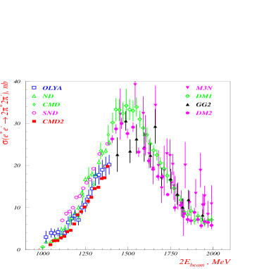
Figure 5: Comparison of data (left figure, see text) and predictions (right figure) obtained using the current Eq.(32) (filled squares) and those of [11] (empty squares) respectively for $\sigma(e^{+}e^{-}\to 2\pi^{+}2\pi^{-})$.

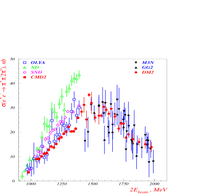
Figure 6: Comparison of data (left figure, see text) and predictions (right figure) obtained using the current Eq.(32) (filled squares) and those of [11] (empty squares) respectively for $\sigma(e^{+}e^{-}\to\pi^{+}\pi^{-}2\pi^{0})$.

In the next step the predictions for the $e^{+}e^{-}\to 2\pi^{+}2\pi^{-}$ (Fig.5) and $e^{+}e^{-}\to\pi^{+}\pi^{-}2\pi^{0}$ (Fig.6) cross sections are compared with data. The plots taken from [19] contain data sets from OLYA [20], ND [21, 22], CMD [23], SND [24], CMD2 [19] plus results of the Orsay [25, 26, 27] and Frascati [28, 29, 30] groups. The data have a typical systematic error of about 15% (shown in plots only for some of the data sets) and we have thus decided not to refit the parameters entering the current as the agreement between the Monte Carlo and the data is acceptable. The modification of the current of [11] we performed leads to significantly better agreement between the theoretical predictions and the data in the mode $e^{+}e^{-}\to\pi^{+}\pi^{-}2\pi^{0}$. Considering the agreement between the $\tau$ decay rates and the prediction we conclude that the model reproduces the data well even if the description of the $\omega$ part of the current is not completely satisfactory.

6 The Monte Carlo program.³

The idea behind the structure of the Monte Carlo program is to allow for a simple addition of new final state modes into the program and for a simple replacement of the current(s) of the existing modes. The program thus exhibits a modular structure. For the generation of the four momenta of the mesons no sophisticated method of a variance reduction was applied. This slows down the generation, but could be accounted for if a faster Monte Carlo generator would be required. It has, however, the advantage of being universal and no change of the variance reduction method is required with each modification of the hadronic current. The process to be simulated by the program in its final stage is $e^{+}e^{-}\rightarrow\gamma\ +\ hadrons$ with an exclusive description of final states, even if till now only $\pi^{+}\pi^{-}$, $2\pi^{0}\pi^{+}\pi^{-}$ and $2\pi^{+}2\pi^{-}$ hadronic final states are implemented. The LL radiative QED corrections were taken into account using structure function method as developed in [31] and limited to the initial emission only. In fact the program can run in one of two modes (chosen by a user) one with collinear radiation and one without it. Hard large angle photon emission is limited to initial state radiation, which is justified by [9] where it was demonstrated for the $\pi^{+}\pi^{-}$ hadronic state that the contribution from the final state emission as well as the initial-final state interference can be reduced to a negligible level by applying suitable cuts.

The generation of the multi particle phase space is based on the following representation of a Lorentz invariant phase space

$${\kern-15.0pt}{\rm dLips}_{n+1}\left(P,k,q_{1},...,q_{n}\right)=\frac{1}{\left(2\pi\right)^{n-1}}\ \ {\rm dQ}_{1}^{2}\ ...\ {\rm dQ}_{n-1}^{2}\ {\rm dLips}_{2}\left(P,Q_{1},k\right)\ {\rm dLips}_{2}\left(Q_{1},Q_{2},q_{1}\right)$$

$${\kern 120.0pt}\ \ ...\ \ {\rm dLips}_{2}\left(Q_{n-2},Q_{n-1},q_{n-2}\right){\rm dLips}_{2}\left(Q_{n-1},q_{n-1},q_{n}\right)\ ,$$ (35)

where $P$ is a total four momentum of the $photon\ +\ hadrons$ state (it is not equal to the sum of the initial $e^{+}e^{-}$ four momenta as we allow for an additional initial collinear emission), $k$ is the photon four momentum, $q_{1}\ ...\ q_{n}$ are the four momenta of the hadrons,

$$Q_{1}=q_{1}+\ ...\ +q_{n}\ \ {\rm and}\ \ Q_{i}=Q_{i-1}-q_{i-1}\ \ {\rm for}\ \ i=2,\ ...\ n-1\ \ ,$$ (36)

and ${\rm dLips}_{2}\left(k_{1},k_{2},k_{3}\right)$ is a two body phase space

$${\rm dLips}_{2}\left(k_{1},k_{2},k_{3}\right)=\frac{1}{32\pi^{2}}\ \frac{\lambda^{\frac{1}{2}}\left(k_{1}^{2},k_{2}^{2},k_{3}^{2}\right)}{k_{1}^{2}}\ {\rm d}\Omega_{3}$$ (37)

with $\lambda\left(a,b,c\right)=a^{2}+b^{2}+c^{2}-2ab-2ac-2bc$ and ${\rm d}\Omega_{3}$ the ${\bf k}_{3}$ solid angle.

The generation flow is the following: first the collinear radiation is generated and a four momentum $P$ of the visible final state is calculated and then boosted to its rest frame(RF) (a CM of the visible final state). This part is omitted in the mode running without collinear emission and then $P$ is a sum of the electron and positron four momenta. In the second step the visible hard photon four momentum is generated. Its energy is generated flat even if the energy distribution is govern by a competition between soft $\sim\frac{1}{E_{\gamma}}$ and a complicated resonant spectrum which depends on details of the hadronic current. Of course this way the generator is not extremely efficient, but it is more universal and will work equally well with all reasonable modifications of the hadronic current. The photon polar angle is generated in $P$ RF with the distribution accounting for collinear emission peaks, which are the same for all hadronic modes as the initial state is ever the same. Its azimuthal angle again is generated with a flat distribution in $P$ RF. Then a chain of a generations of $Q_{i}^{2}\ ,\ i=2,...,n-1$ follows ($Q_{1}$ is fixed when we generate the photon four momentum). They are generated flat within their allowed limits

$$\left(\sum_{k=i}^{n}m_{k}\right)^{2}\ <\ Q_{i}^{2}\ <\ \left(Q_{i-1}^{(0)}-m_{i-1}\right)^{2}$$ (38)

where $Q_{i}^{(0)}$ is a zeroth component of the $Q_{i}$ four momentum. At the end a generation of the solid angles $\Omega_{i},\ i=1,...,n-1$ follows. They are generated flat ( $\Omega_{i}$ in $Q_{i}$ RF). All generated four momenta are then transformed with the use of the proper boosts and rotations into the CM system of the initial $e^{+}e^{-}$ particles. The distribution of the events $\sim|{\cal M}|^{2}$, where ${\cal M}$ is a matrix element of a given process is obtained by means of the rejection method. The cross section is calculated using Eq.(5) both for weighted and unweighted event samples. The unweighted events are stored in a file when requested.

Let us now discuss the cuts, which reduce the contribution of the final state emission to the cross section to a negligible level allowing thus for extraction of $R(Q^{2})$ from the measurement of the $e^{+}e^{-}\to\ hadrons\ +\gamma$ cross section. We recall that in [9] it was shown that the following set of angular cuts

$${\rm cuts1:}\ \ \ \ \ \ \ \ \ \ \left(7^{\circ}<\theta_{\gamma}<20^{\circ}\ \ \ \ \ or\ \ \ \ \ 160^{\circ}<\theta_{\gamma}<173^{\circ}\right)\ \ \ and\ \ \ 30^{\circ}<\theta_{\pi}<150^{\circ}\ ,$$ (39)

( $\theta_{\gamma}$ ($\theta_{\pi}$ ) is the photon (pion) polar angle) fulfils this requirement for the $e^{+}e^{-}\to\pi^{+}\pi^{-}\gamma$ cross section. It reduces, however, the observed cross section significantly. This starts to become dramatic, when one runs at energies well above 1 GeV. The following set of cuts

$${\rm cuts2:}\ \ \ \ \ \ \ \ \ \ \left(7^{\circ}<\theta_{\gamma}<20^{\circ}\ \ \ and\ \ \ 30^{\circ}<\theta_{\pi}<173^{\circ}\right)$$ (40)

$${\kern-40.0pt}or\ \ \ \left(160^{\circ}<\theta_{\gamma}<173^{\circ}\ \ \ and\ \ \ 7^{\circ}<\theta_{\pi}<150^{\circ}\right)\ ,$$

also reduces the contribution from final state radiation to a negligible level due to the fact that the pions and photon are well separated as in the previous case.

Figure 7: The differential $e^{+}e^{-}\to 4\pi\gamma$ cross sections at beam energy 1.5 GeV with minimal photon energy equal 0.1 GeV with no cuts on pions angles and $7^{\circ}<\theta_{\gamma}<173^{\circ}$ ( no cuts) and two sets of angular cuts Eq.(39) (with cuts1) and Eq.(40) (with cuts2), where $q\equiv\sqrt{Q^{2}}$ is an invariant mass of the $4\pi$ system.

Figure 8: The differential $e^{+}e^{-}\to 4\pi\gamma$ cross sections at beam energy 5 GeV with minimal photon energy equal 0.2 GeV with no cuts on pions angles and $7^{\circ}<\theta_{\gamma}<173^{\circ}$( no cuts) and angular cuts of Eq.(40) (with cuts2), where $q\equiv\sqrt{Q^{2}}$ is an invariant mass of the $4\pi$ system.

At the same time the cross section reduction is much smaller, especially for higher beam energies and higher energies of the observed photons. The effect of the two sets of cuts on the cross sections with four pions in the final state is presented in Fig.7 for $2E_{beam}$ = 3 GeV. For higher beam energies the effect of the cross section reduction is much higher and at 2 $E_{beam}$ = 10 GeV the cross sections for cuts specified in Eq.(39) is reduced almost to zero. For the cuts specified in Eq.(40) the results are presented in Fig.8 and the reduction remains tolerable.

$$\begin{array}[]{||c||c||c|c||}\hline\cr&&\vrule\lx@intercol\hfil{\rm Event~{}rates}\hfil\lx@intercol\vrule\lx@intercol\\ \hline\cr\sqrt{s}&{\rm Integrated~{}luminosity},{\rm fb}^{-1}&\ \ \ 2\pi^{+}2\pi^{-}\gamma&\ \ \ 2\pi^{0}\pi^{+}\pi^{-}\gamma\\ \hline\cr\hline\cr\ 1\ {\rm GeV}&1&1.04\cdot 10^{4}&1.13\cdot 10^{4}\\ \hline\cr\hline\cr\ 3\ {\rm GeV}&1&4.66\cdot 10^{4}&5.72\cdot 10^{4}\\ \hline\cr\hline\cr\ 10\ {\rm GeV}&100&1.86\cdot 10^{5}&2.33\cdot 10^{5}\\ \hline\cr\end{array}$$

Table 5: Estimated number of radiative events $e^{+}e^{-}\to\ 4\pi\ +\ \gamma$ for different center of mass energies. The minimal photon energy is: 0.05 GeV (first row), 0.1 GeV (second row), 0.2 GeV (third row). The angular cuts of Eq.(40) were applied.

From Fig.8 one concludes that one can measure $R(Q^{2})$ at a B factory in the interesting region of $\sqrt{Q^{2}}$ between 1 GeV and 2.5 GeV through measuring the $e^{+}e^{-}\to 4\pi\gamma$ cross section using Eq.(8). This measurement should have an an accuracy much better then 15 % , which is now the typical experimental error in that $Q^{2}$ region, allowing for a reduction of the error in the calculation of the photon vacuum polarization. From Table 5 it is clear that the error would be dominated by systematics and not by statistics.

One may even restrict photon and pions detection angles to the central region, e.g. $25^{\circ}<\theta_{\gamma}<155^{\circ}$ and $30^{\circ}<\theta_{\pi}<150^{\circ}$ respectively if a minimal angle of $20^{\circ}$ between photon and charged and neutral pions is required in order to suppress final state radiation and to clearly separate neutral pions and the photon. With this cut one obtains ($\sqrt{s}=10\ GeV$ and ${\cal L}=100\ fb^{-1}$ ) a rate of $1.17\cdot 10^{5}$ events with $2\pi^{+}2\pi^{-}\gamma$ and $1.53\cdot 10^{5}$ events with $2\pi^{0}\pi^{+}\pi^{-}\gamma$.

Figure 9: The effect of the collinear radiation on the differential $e^{+}e^{-}\to 4\pi\gamma$ cross sections at beam energy 0.5 GeV (left picture) and 5 GeV (right picture) with minimal photon energy equal to 0.05 and 0.2 GeV correspondingly. In the mode with collinear radiation minimal invariant masses of the $4\pi\ +\ \gamma$ systems of 0.95 GeV and 9.5 GeV were required. $q\equiv\sqrt{Q^{2}}$ denotes the invariant mass of the $4\pi$ system.

Additional collinear emission always present in the real experiment reduces slightly the cross sections as shown in Figs.9 for two different modes and two different beam energies. Its actual size depends on the cuts on the invariant mass of the $4\pi\ +\ \gamma$ system. The effect is similar for different energies and for both charge modes.

7 Summary.

A precise value of the cross section for hadron production in electron positron annihilation at low energies is one of the important ingredients for a reliable prediction of the anomalous magnetic of the muon and the electromagnetic coupling at high energies. As an alternative to a direct measurement at the relevant energy one may use initial state radiation to reduce the effective energy of electron positron colliders, exploiting the large luminosity of “factories” and accessing thus a continuum of hadronic final states.

With this motivation a Monte Carlo generator has been constructed to simulate the reaction $e^{+}e^{-}\to\gamma+4\pi$, where the photon is assumed to be observed in the detector. The hadronic matrix element has been taken from [11]. Isospin relations between the amplitudes governing $\tau$ decays into four pions and electron positron annihilation into four pions have been found which allow to determine all four modes after the amplitude for the $\pi^{+}\pi^{-}2\pi^{0}$ channel has been fixed. The kinematic breaking of these isospin relations as a consequence of the $\pi^{-}$ – $\pi^{0}$ mass difference has also been investigated.

The program is constructed in analogy to the one [9] simulating $e^{+}e^{-}\to\gamma+2\pi$. However, it does not include final state radiation from the charged pions. Additional collinear photon radiation has been incorporated with the technique of structure functions. Predictions are presented for cms energies of 1GeV, 3GeV and 10GeV, corresponding to the energies of DA$\Phi$NE, BEBC and of $B$-meson factories.

Even after applying realistic cuts the event rates are sufficiently high to allow for a precise measurement of $R(Q^{2})$ in the region of $Q$ between approximately 1GeV and 2.5GeV.

The model predictions are compared to recent data from electron positron colliders. Once more accurate data become available, the modular structure of the program will allow for modification of replacement of the hadronic current in a simple way.

Acknowledgments. The work by H.C. was supported by BMBF-POL-239-96, the work by J.K. by BMBF under grant BMBF-057KA92P. H.C. is grateful for the support and the kind hospitality of the Institut für Theoretische Teilchenphysik of the Karlsruhe University, where this work was carried out.

Appendix: The description of the hadronic current.

In this appendix we give a complete definition of the hadronic current used in this paper. Recalling Eq.(32)

$$\Gamma^{\mu}_{\rho^{0}\rightarrow 2\pi^{0}\pi^{+}\pi^{-}}=\Gamma^{\mu}_{a_{1}}+\Gamma^{\mu}_{f_{0}}+\Gamma^{\mu}_{\omega}\ ,$$ (41)

we will define here its ingredients.

Denoting the pions four momenta as follows: $q_{1}(\pi^{0}),q_{2}(\pi^{0}),q_{3}(\pi^{-})\ \ {\rm and}\ \ q_{4}(\pi^{+})$ one gets the following contribution from the part containing an $a_{1}$ exchange

$$\Gamma^{\mu}_{a_{1}}\left(q_{1},q_{2},q_{3},q_{4}\right)=$$

$$\tilde{\Gamma}^{\mu}_{a_{1}}(q_{3},q_{2},q_{1},q_{4})+\tilde{\Gamma}^{\mu}_{a_{1}}(q_{3},q_{1},q_{2},q_{4})-\tilde{\Gamma}^{\mu}_{a_{1}}(q_{4},q_{2},q_{1},q_{3})-\tilde{\Gamma}^{\mu}_{a_{1}}(q_{4},q_{1},q_{2},q_{3}).$$ (42)

The structure of this current follows from the form of the Lagrangian of the $\rho a\pi$ ($\sim\vec{a}\cdot\left(\vec{\pi}\times\vec{\rho}\right)$ ) and $\rho\pi\pi$ ($\sim\vec{\rho}\cdot\left(\vec{\pi}_{1}\times\vec{\pi}_{2}\right)$ ) interactions and the function $\tilde{\Gamma}^{\mu}_{a}$ is defined as [11]

$$\tilde{\Gamma}^{\mu}_{a_{1}}(q_{1},q_{2},q_{3},q_{4}) = C_{1}\ \ T_{\rho}\left(Q^{2}\right)\ \ \Gamma^{\mu\nu}\left(Q,Q-q_{1}\right)$$ (43)

$$BW_{a_{1}}\left((Q-q_{1})^{2}\right)\ \ \Gamma_{\nu\lambda}\left(Q-q_{1},Q-q_{1}-q_{2}\right)$$

$$BW_{\rho}\left((q_{3}+q_{4})^{2}\right)\ \ \Gamma_{1}^{\lambda}(q_{3}-q_{4})\ ,$$

where we have followed the notation of [11]; $Q=q_{1}+q_{2}+q_{3}+q_{4}$.

Assuming that $q_{1}^{2}=q_{2}^{2}=q_{3}^{2}=q_{4}^{2}=m_{\pi}^{2}$ i.e. that pions have equal masses one finds

$${\kern-30.0pt}\tilde{\Gamma}^{\mu}_{a_{1}}(q_{1},q_{2},q_{3},q_{4})=$$

$$C_{1}\ f_{\rho\pi\pi}\left((q_{3}+q_{4})^{2}\right)\ f_{a_{1}\rho\pi}(Q^{2},(Q-q_{1})^{2})\ f_{a_{1}\rho\pi}((Q-q_{1})^{2},(q_{3}+q_{4})^{2})$$

$$T_{\rho}\left(Q^{2}\right)\ \ BW_{a_{1}}\left((Q-q_{1})^{2}\right)\ \ BW_{\rho}\left((q_{3}+q_{4})^{2}\right)$$

$${\kern-7.0pt}\left[(q_{3}-q_{4})^{\mu}+q_{1}^{\mu}\frac{q_{2}(q_{3}-q_{4})}{(Q-q_{1})^{2}}-Q^{\mu}\left(\frac{(q_{1}+q_{2})(q_{3}-q_{4})}{Q^{2}}+\frac{(Qq_{1})(q_{2}(q_{3}-q_{4}))}{Q^{2}(Q-q_{1})^{2}}\right)\right]\ ,$$ (44)

where $f_{\rho\pi\pi}$ and $f_{a_{1}\rho\pi}$ describe $\rho\pi\pi$ and $a_{1}\rho\pi$ vertices appropriately while $T_{\rho}$, $BW_{a_{1}}$ and $BW_{\rho}$ are $\rho$, $a_{1}$ and again $\rho$ propagators. The different choice of the authors of [11] for two $\rho$ propagators comes from the fact that $\rho$ couples in a different way in the two cases and the ’propagators’ absorb in fact some parts of the couplings. The normalization constant $C_{1}=\frac{2\ \sqrt{6}}{f_{\pi}^{2}}$ was chosen to give the proper chiral limit of the current. The form factors were chosen to be constant

$\left[f_{\rho\pi\pi}\left((q_{3}+q_{4})^{2}\right)\ f_{a_{1}\rho\pi}(Q^{2},(Q-q_{1})^{2})\ f_{a_{1}\rho\pi}((Q-q_{1})^{2},(q_{3}+q_{4})^{2})\right]=0.38$,

and the validity of that assumption was proved [11] in a limited range of $Q^{2}$

($1.1\ {\rm GeV}\ <\sqrt{Q^{2}}\ <\ 2.2\ {\rm GeV}$ ).

The contribution to the current from $f_{0}$ exchange reads

$$\Gamma^{\mu}_{f_{0}}(q_{1},q_{2},q_{3},q_{4}) =$$ (45)

$${\kern-20.0pt}C_{2}\ f_{\rho\rho f_{0}}\left(Q^{2},(q_{3}+q_{4})^{2},(q_{1}+q_{2})^{2}\right)\ f_{\rho\pi\pi}\left((q_{3}+q_{4})^{2}\right)\ f_{f_{0}\pi\pi}\left((q_{1}+q_{2})^{2}\right)$$

$$T_{\rho}\left(Q^{2}\right)\ T_{\rho}\left((q_{3}+q_{4})^{2}\right)\ BW_{f_{0}}\left((q_{1}+q_{2})^{2}\right)$$

$$\left[(q_{3}-q_{4})^{\mu}-Q^{\mu}\frac{Q(q_{3}-q_{4})}{Q^{2}}\right]\ ,$$

where $f_{\rho\rho f_{0}}$ and $f_{f_{0}\pi\pi}$ describe $\rho\rho f_{0}$ and $f_{0}\pi\pi$ vertices appropriately, while $BW_{f_{0}}$ is an $f_{0}$ propagator.

Again $C_{2}=-\frac{3\ \sqrt{6}}{f_{\pi}^{2}}$ follows from the chiral limit and the form factors are kept constant

$f_{\rho\rho f_{0}}\left(Q^{2},(q_{3}+q_{4})^{2},(q_{1}+q_{2})^{2}\right)\ f_{\rho\pi\pi}\left((q_{3}+q_{4})^{2}\right)\ f_{f_{0}\pi\pi}\left((q_{1}+q_{2})^{2}\right)=0.38\ .$

The contribution coming from so called anomalous (containing $\omega$ exchange) part of the current reads

$$\Gamma^{\mu}_{\omega}(q_{1},q_{2},q_{3},q_{4})=\frac{g_{\omega}}{\sqrt{2}}\ 1475.98\ {\rm GeV}^{-3}\ 12.924\ {\rm GeV}^{-1}\ 0.266\ m_{\rho}^{2}$$

$${\kern-25.0pt}\left[q_{1}^{\mu}F_{1}(q_{1},q_{2},q_{3},q_{4})+q_{2}^{\mu}F_{1}(q_{2},q_{1},q_{3},q_{4})+q_{3}^{\mu}F_{2}(q_{1},q_{2},q_{3},q_{4})-q_{4}^{\mu}F_{2}(q_{1},q_{2},q_{4},q_{3})\right]\ ,$$ (46)

where

$${\kern-25.0pt}F_{1}(q_{1},q_{2},q_{3},q_{4})=BW_{\rho,\omega}(Q^{2},(Q-q_{2})^{2})\left[(q_{3}(Q-q_{2}))\ (q_{2}q_{4})-(q_{4}(Q-q_{2}))\ (q_{2}q_{3})\right]$$ (47)

$${\rm and}$$

$${\kern-25.0pt}F_{2}(q_{1},q_{2},q_{3},q_{4})=BW_{\rho,\omega}(Q^{2},(Q-q_{2})^{2})\left[(q_{4}(Q-q_{2}))\ (q_{1}q_{2})-(q_{1}(Q-q_{2}))\ (q_{2}q_{4})\right]$$

$${\kern 55.0pt}+BW_{\rho,\omega}(Q^{2},(Q-q_{1})^{2})\left[(q_{4}(Q-q_{1}))\ (q_{1}q_{2})-(q_{2}(Q-q_{1}))\ (q_{1}q_{4})\right]$$ (48)

and $g_{\omega}=1.55$. It is changed from its original value $g_{\omega}=1.4$ in [11] to reproduce the $\tau$ decay rates $\tau^{-}\to\nu_{\tau}2\pi^{-}\pi^{+}\pi^{0}$ and $\tau^{-}\to\nu_{\tau}\pi^{-}\omega\left(\pi^{-}\pi^{+}\pi^{0}\right)$.

For completeness we list here all propagators [11] required for the current:

$$T_{\rho}\left(Q^{2}\right)=\frac{BW_{3}(Q^{2},m_{\rho},\Gamma_{\rho})+\beta_{1}BW_{3}(Q^{2},m_{\rho_{1}},\Gamma_{\rho_{1}})+\beta_{2}BW_{3}(Q^{2},m_{\rho_{2}},\Gamma_{\rho_{2}})}{1+\beta_{1}+\beta_{2}}\ ,$$ (49)

with

$$BW_{3}(Q^{2},m_{\rho},\Gamma_{\rho})=\frac{m_{\rho}^{2}}{m_{\rho}^{2}-Q^{2}-i\Gamma_{\rho}m_{\rho}\sqrt{\frac{m_{\rho}^{2}}{Q^{2}}\left[\frac{Q^{2}-4m_{\pi}^{2}}{m_{\rho}^{2}-4m_{\pi}^{2}}\right]^{3}}}$$ (50)

and the numerical values set to

$$m_{\pi}=0.14\ {\rm GeV}$$

$$m_{\rho}=0.773\ {\rm GeV}\ \ \Gamma_{\rho}=0.145\ {\rm GeV}$$

$$m_{\rho_{1}}=1.35\ {\rm GeV}\ \ \Gamma_{\rho_{1}}=0.3\ {\rm GeV}\ \ \beta_{1}=0.08$$

$$m_{\rho_{2}}=1.7\ {\rm GeV}\ \ \Gamma_{\rho_{2}}=0.235\ {\rm GeV}\ \ \beta_{2}=-0.0075\ \ ;$$ (51)

$$BW_{\rho}\left(Q^{2}\right)=\frac{BW_{3}(Q^{2},m_{\rho},\Gamma_{\rho})+\beta BW_{3}(Q^{2},\tilde{m}_{\rho_{1}},\tilde{\Gamma}_{\rho_{1}})}{1+\beta}\ \ ,$$ (52)

with

$$\tilde{m}_{\rho_{1}}=1.37\ {\rm GeV}\ \ \tilde{\Gamma}_{\rho_{1}}=0.510\ {\rm GeV}\ \ \beta=-0.145\ ;$$ (53)

$$BW_{a_{1}}\left(Q^{2}\right)=\frac{m_{a_{1}}^{2}}{m_{a_{1}}^{2}-Q^{2}-i\Gamma_{a_{1}}m_{a_{1}}\frac{g(Q^{2})}{g(m_{a_{1}}^{2})}}\ ,$$ (54)

where

$$g(Q^{2})=1.623\ Q^{2}+10.38-\frac{9.32}{Q^{2}}+\frac{0.65}{(Q^{2})^{2}}\ \ \ \ {\rm for}\ \ \ \ Q^{2}>(m_{a_{1}}+m_{\pi})^{2}$$

$$g(Q^{2})=4.1\ \left(Q^{2}-9m_{\pi}^{2}\right)^{3}\left[1-3.3\left(Q^{2}-9m_{\pi}^{2}\right)+5.8\left(Q^{2}-9m_{\pi}^{2}\right)^{2}\right]$$

$${\kern 100.0pt}{\rm for}\ \ Q^{2}<(m_{a_{1}}+m_{\pi})^{2}$$ (55)

and

$$m_{a_{1}}=1.251\ {\rm GeV}\ \ \Gamma_{a_{1}}=0.599\ {\rm GeV}\ ;$$ (56)

$$BW_{f_{0}}\left(Q^{2}\right)=\frac{m_{f_{0}}^{2}-im_{f_{0}}\Gamma_{f_{0}}}{m_{f_{0}}^{2}-Q^{2}-im_{f_{0}}\Gamma_{f_{0}}}$$ (57)

with

$$m_{f_{0}}=1.3\ {\rm GeV}\ \ \Gamma_{f_{0}}=0.6\ {\rm GeV}\ ;$$ (58)

$$BW_{\rho,\omega}(Q^{2},Q_{1}^{2}) = \left[\frac{1}{m_{\rho}^{2}-Q^{2}-im_{\rho}\Gamma_{\rho}}+\sigma\frac{1}{m_{\rho\prime}^{2}-Q^{2}-im_{\rho\prime}\Gamma_{\rho\prime}}\right]\frac{1}{m_{\omega}^{2}-Q_{1}^{2}-im_{\omega}\Gamma_{\omega}}$$ (59)

$${\kern-20.0pt}\left[\ \theta\left((2.2\ {\rm GeV})^{2}-Q^{2}\right)+\theta\left(Q^{2}-(2.2\ {\rm GeV})^{2}\right)\left(\frac{\left(2.2\ {\rm GeV}\right)^{2}}{Q^{2}}\right)^{2}\right]$$

with

$$m_{\rho\prime}=1.7\ {\rm GeV}\ \ \Gamma_{\rho\prime}=0.26\ {\rm GeV}\ \ \sigma=-0.1$$

$$m_{\omega}=0.782\ {\rm GeV}\ \ \Gamma_{\omega}=0.0085\ {\rm GeV}\ .$$ (60)

An additional suppression compared to [11] above $Q^{2}=\left(2.2\ {\rm GeV}\right)^{2}$ was introduced. This modification prevents the unphysical growth of the cross section for very large $Q^{2}$, which originates from the momentum dependent couplings in Eq.(46)-Eq.(48).

References

[1] H.B. Thacker and J.J. Sakurai, Phys. Lett. 36B
(1971) 103.