CERN-TH/2000-253

In a simplified model we study the hadronization of quark matter in an expanding fireball, in particular the approach to a final hadronic composition in equilibrium. Ideal hadron gas equilibrium constrained by conservation laws, the fugacity parametrization, as well as linear and non-linear coalescence approaches are recognized as different approximations to this in-medium quark fusion process. It is shown that color confinement requires a dependence of the hadronization cross section on quark density in the presence of flow (dynamical confinement).

To appear in the Proc. of the Strange Matter 2000 Conference

1 Introduction

Since flavor composition, in particular strangeness enhancement had been suggested as a possible signature of quark matter formation in heavy-ion collisions, there is a continuing attention to the question of hadronic and quark level equilibrium in these reactions [2, 3]. Recent claims of describing data at AGS as well as at CERN SPS by hadronic equilibrium (i.e. using a common volume, temperature and only chemical potentials of conserved quantities for the computation of hadron numbers) satisfactorily [4, 5, 6] led to some discrepancy: the total reaction time at SPS energy is too short for achieving hadronic equilibrium by hadronic conversion processes alone. Experimental data are well described, but poorly understood. After the “go and find it” period now we are at the “sit down and think” stage.

There are also several non-equilibrium approaches to this problem ranging from the use of phenomenological parameters on the hadronic level (fugacities) [7] through linear [8] and nonlinear (constrained) coalescence models [9], and mixed quark-hadron chemistry [10] up to very detailed microscopic simulations of the hadronization (parton cascades [11, 12] VENUS [13], HIJING [14], RQMD [15, 16], UrQMD [17, 18], string model [19, 20, 21], chromodielectric model [22]). The basic physical concepts of these approaches do not include hadronic equilibrium; it might only be reached in course of time.

The purpose of this talk is to understand the near-equilibrium hadronic result in terms of quark number evolution. We consider the simplest possible process on the constituent level: $A+B\longleftrightarrow C.$

In such a process the energy-impulse balance is assumed to be satisfied by the surrounding medium, we are interested in the time evolution of the number of final state products $N_{C}(t)$. The equilibrium number of precursors $N_{A,eq}$ and $N_{B,eq}$ - in a quark matter scenario - will be taken as zero. The initial state is assumed to be far from this equilibrium, it is oversaturated by $A$ and $B$ with no $C$ particles at all in the beginning. As the reaction proceeds there will be $C$ type particles (hadrons) produced. The cross section for such a reaction at a first glance can be taken as constant, but temperature and reaction volume must be considered as time dependent quantities. We shall point out, however, that the assumption of constant cross sections actually contradicts to the confinement principle in quark matter scenarios with transverse flow, so in that case the hadronization cross section has to be quark density dependent. This extra dependency, not derivable from perturbative or lattice QCD so far, will be referred as “dynamical confinement” in this paper.

2 Chemistry

In the chemical approach to hadronization all particle numbers are time dependent. A general reaction can be characterized by stochiometric coefficients $\alpha_{i}^{(r)}$ describing particle number changes in a given reaction $(r)$ in a fashion arranged to zero:

$$\sum_{i}\alpha_{i}^{(r)}A_{i}=0,$$ (1)

where $A_{i}$ symolically denotes one particle of type $i$. In this arrangement the $\alpha_{i}^{(r)}$-s can be negative as well as positive integers. (For the simple quark fusion process $A+B\longleftrightarrow C$ one applies $\alpha_{A}=\alpha_{B}=1,\alpha_{C}=-1$.)

The decisive quantity with respect to approaching chemical equilibrium is the activity of a reaction,

$$x^{(r)}=\sum_{i}\alpha_{i}^{(r)}\frac{\mu_{i}}{T}.$$ (2)

It describes the (un)balance of gain and loss terms. Rate equations add up contributions from several reaction channels,

$$\dot{N}_{i}=\sum_{(r)}\alpha_{i}^{(r)}R^{(r)}\left(1-e^{x^{(r)}}\right).$$ (3)

Here the factors $R^{(r)}$ depend on numbers of other particles, cross sections and volume. Due to known (e.g. adiabatic) expansion a relation between volume $V$ and temperature $T$ is given. In chemical equilibrium $x^{(r)}=0$ for each reaction,

$$\sum_{i}\alpha_{i}^{(r)}\mu_{i}=0,$$ (4)

so there are linear constraints for the chemical potentials $\mu_{i}$ as many as reaction channels. If this is less than the number of particle sorts, the equilibrium state is undetermined. If this is greater than the number of particle sorts, the reactions cannot be all independent: there are conserved quantities. In this latter case all $\mu_{i}$ can be expressed by a few numbers corresponding to these conserved quantities. This is the constrained equilibrium.

Denoting the conserved quantities by $Q_{a}$ and the corresponding charge of the i-th particle sort by $q_{i,a}$, we obtain

$$\sum_{i}q_{i,a}\dot{N}_{i}=0.$$ (5)

Substituting the rate equations (3) we get

$$\sum_{i}\sum_{r}\alpha_{i}^{(r)}q_{i,a}R^{(r)}\left(1-e^{x^{(r)}}\right)=0.$$ (6)

Since this holds at any instant of an out of equilibrium evolution, the double sum vanishes for arbitrary values of reaction activities $x^{(r)}$. Exchanging the order of summation over particle types $i$ and reaction channels $r$, and taking into account that all $R^{(r)}$ factors are positive, we conclude that the considered charges are conserved in each reaction:

$$\sum_{i}\alpha_{i}^{(r)}q_{i,a}=Q^{(r)}_{a}=0.$$ (7)

In this case we can redefine the chemical potentials as

$$\mu_{i}=\sum_{a}q_{i,a}\mu_{a}+\tilde{\mu}_{i},$$ (8)

without changing the activities:

$$x^{(r)}=\sum_{i}\sum_{a}\alpha_{i}^{(r)}\frac{q_{i,a}\mu_{a}}{T}+\sum_{i}\alpha_{i}^{(r)}\frac{\tilde{\mu}_{i}}{T}.$$ (9)

Since the first sum vanishes due to eq.(7), chemical equilibrium is equivalent to

$$\sum_{i}\alpha_{i}^{(r)}\frac{\tilde{\mu}_{i}}{T}=0.$$ (10)

For a well-determined or overdetermined system the only equilibrium solution is given by $\tilde{\mu}_{i}=0.$ In this (constrained) equilibrium state the original chemical potentials are a linear combination of a few $\mu_{a}$-s, associated to conserved charges, (cf. eq.(8))

$$\mu_{i,eq}=\sum_{a}q_{i,a}\mu_{a}.$$ (11)

Whether this chemical equilibrium state can be reached in a finite time depends on the rates $R^{(r)}$ and activities $x^{(r)}$.

3 A simple model: A + B $\longleftrightarrow$ C

In the case of only one reaction channel, $A+B\longleftrightarrow C,$ we denote the equilibrium ratio by

$$R_{{\rm eq}}=\frac{N_{A,{\rm eq}}N_{B,{\rm eq}}}{N_{C,{\rm eq}}}.$$ (12)

Since $\alpha_{A}=\alpha_{B}=1$ and $\alpha_{C}=-1$ for this very reaction, we have $\dot{N}_{A}=\dot{N}_{B}=-\dot{N}_{C}$. From this two conservation laws follow,

$$N_{A}+N_{C}=N_{A}(0)=N_{0},$$ (13)

$$N_{B}+N_{C}=N_{B}(0)=N_{0}.$$ (14)

For considering an evolution towards equilibrium the specific rate, $\nu=\langle\sigma v\rangle/V,$ is a useful quantity. It occurs in the rate equation

$$\dot{N}_{C}=\nu\left(N_{A}N_{B}-R_{eq}N_{C}\right).$$ (15)

Substituting the conservation laws (13,14) we arrive at

$$\dot{N}_{C}=\nu\left((N_{0}-N_{C})(N_{0}-N_{C})-R_{eq}N_{C}\right).$$ (16)

This rate is vanishing for the particle numbers $N_{C}=N_{\pm}$ with

$$N_{\pm}=R_{eq}/2+N_{0}\pm\sqrt{R_{eq}^{2}/4+R_{eq}N_{0}}.$$ (17)

Here $N_{-}$ is a stable, $N_{+}$ is an unstable equilibrium point. For an adiabatic expansion $R_{eq}=const.$ for constituent hadrons (those with mass $m_{C}=m_{A}+m_{B}$). The simple rate equation (16) can be solved analytically with the result

$$\int_{N_{C}(0)}^{N_{C}(\infty)}\frac{dN_{C}}{(N_{C}-N_{+})(N_{C}-N_{-})}=\int_{t_{0}}^{t_{br}}\nu dt=r.$$ (18)

Here $t_{0}$ is the initial time, when the fireball contains no hadrons, $N_{C}(0)=0$. $t_{br}$ is the break-up time, beyond which no chemical reactions (even no particle collisions) occur. In some cases it is large compared to characteristic times and can be approximated by infinity. The solution can be written as

$$N_{C}(\infty)=N_{+}N_{-}\frac{1-K}{{N_{+}}-K{N_{-}}}$$ (19)

with

$$K=\exp\left(-(N_{+}-N_{-})r\right).$$ (20)

Here $N_{-}$ is the constrained equilibrium value, achieved for $K=0$. There are two alternative forms of this relation derived by using $N_{+}N_{-}=N_{0}^{2}$. The first one is the coalescence form,

$$N_{C}(\infty)=N_{0}^{2}\frac{1-K}{N_{+}-KN_{-}}=C(K,N_{0})N_{A}(0)N_{B}(0),$$ (21)

the second one is the equilibrium form,

$$N_{C}(\infty)=N_{-}\frac{1-K}{1-K(N_{-}/N_{0})^{2}}=\gamma_{C}N_{C,{\rm eq}}.$$ (22)

In particular $N_{C}(\infty)=N_{-}$ in the $K=0$ (infinite rate) case. On the other hand in the case of confinement $R_{eq}=0$, from which $N_{+}=N_{-}=N_{0}$ and $K=1$ follow.

For $(N_{+}-N_{-})$ small (${\cal O}(R_{eq})$), but non-zero the precursors are already hadronic, but suppressed in the equilibrium state. Then we expect, that in the $R_{{\rm eq}}\rightarrow 0$ limit the precursors $A$ and $B$ are no more present in the final mixture. This is, however, insufficient for the quark matter hadronization scenario, because the above limit does not automatically lead to an absence of $A$ and $B$ particles in the final state, if the expansion is dramatic enough. We describe this phenomenon in the followings.

Let us expand $K$ in terms of $(N_{+}-N_{-})$ which is in the same order of magnitude as $R_{{\rm eq}}\rightarrow 0$. We get

$$K=\exp(-(N_{+}-N_{-})r)\approx 1-r(N_{+}-N_{-}),$$ (23)

and the final hadron number becomes

$$N_{C}(\infty)=N_{0}\frac{rN_{0}}{1+rN_{0}},$$ (24)

leaving us with a non-vanishing precursor number

$$N_{A}(\infty)=N_{B}(\infty)=N_{0}\frac{1}{1+rN_{0}}.$$ (25)

Eq. (24) has different readings. For small $r$ it is close to the result of linear coalescence models

$$N_{C}(\infty)=rN_{0}^{2}.$$ (26)

(Note that $N_{A}(0)=N_{B}(0)=N_{0}$.) ALCOR uses extra modification factors $b_{A}$ and $b_{B}$ in the coalescence rate

$$N_{C}(\infty)=rb_{A}b_{B}N_{0}^{2}.$$ (27)

To start with it seems to be rather similar to the coalescence picture. Due to conservation of quark number during an – supposedly rapid – hadronization, however, ALCOR obtains

$$N_{C}(\infty)=rb_{A}b_{B}N_{0}^{2}=\frac{r}{1+rN_{0}}N_{0}^{2}$$ (28)

and determines the factors $b_{i}$ accordingly

$$b_{A}=b_{B}=\frac{1}{\sqrt{1+rN_{0}}}.$$ (29)

It leads exactly to the constrained equilibrium result in the infinite integrated specific rate limit $rN_{0}\rightarrow\infty$ (then $b_{A}=b_{B}\approx 1/\sqrt{rN_{0}}$):

$$N_{C}(\infty)=N_{0},\qquad\qquad N_{A}(\infty)=N_{B}(\infty)=0.$$ (30)

In this limit the precursor numbers approach zero, and the above discussion can be applied for quark matter hadronization. Or, reversing the argument, we conclude that for quark matter hadronization $r$ has to diverge in order to agree with confinement in the end stage. (This fact is nonetheless hidden in the thermodynamical limit with infinite quark number $N_{0}\rightarrow\infty$.)

Finally the chemistry approach gives the interpretation of the fugacity due to

$$N_{C}(\infty)=N_{0}^{2}\frac{r}{1+rN_{0}}=\gamma_{C}N_{0}.$$ (31)

In fact the relationship between these approaches is more pronounced by inspecting chemical potentials instead of final numbers. In the discussed simple case the chemical potential of the (final state) hadron is given by

$$\frac{\mu_{C}}{T}=\log\frac{N_{C}(\infty)}{N_{C,eq}}.$$ (32)

Substituting our result for $N_{C}(\infty)$ it splits to contributions with different physical meanings:

$$\frac{\mu_{C}}{T}=\log\frac{N_{-}}{N_{C,eq}}\,+\,\log\frac{N_{C}(\infty)}{N_{-}}=\frac{q_{C,1}\mu_{1}+q_{C,2}\mu_{2}}{T}+\log\gamma_{C}.$$ (33)

The conserved quantities (charges) carried by the hadron $C$ are those involved in the identities respected by the rate equations, $N_{A}(t)+N_{C}(t)=N_{A}(0)=N_{0}$ and $N_{B}(t)+N_{C}(t)=N_{B}(0)=N_{0}$. In this case $q_{C,1}=1$ and $q_{C,2}=1$, respectively. The fugacity parameter (as used by Rafelski et al.) is the remaining part of the formula, in equilibrium it approaches one: $\gamma_{C}=1$.

We note here that the ALCOR approach (constrained coalescence) leads to the equilibrium result only if a single reaction channel is considered, like in the case discussed in the present paper. For several, competing channels the relative hadron ratios are different for ALCOR and constrained equilibrium. This best can be seen by inspecting the corresponding $\mu_{i}$ chemical potentials to the pre resonance decay hadron numbers as a function of strangeness in the ALCOR simulation. Slight deviations from the perfect straight lines, which would mark the constrained equilibrium in the ideal case, can be observed in particular for multiply strange anti-baryons (cf. Fig.1).

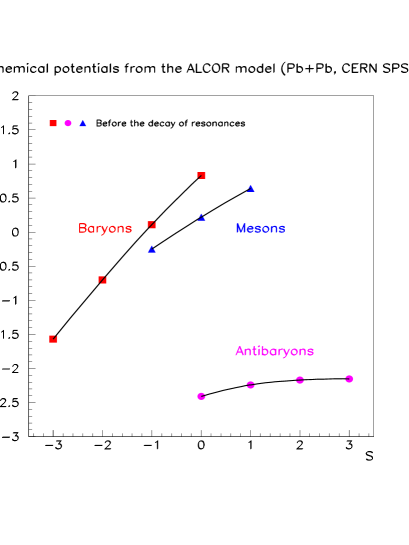
Figure 1: Equivalent chemical potentials of composite hadrons before resonance decay obtained in ALCOR as a function of the strangeness. Linearity corresponds to hadronic equilibrium.

4 Expansion effects

We continue by obtaining the integrated specific rate, $r,$ for different expansion scenarios. This quantity depends not only on cross section(s) – first assumed to be constant and later density dependent – but also on the expansion and cooling of the reaction zone. We consider here two cases: one dimensional expansion with a rather relativistic equation of state and three dimensional expansion of a massive, non-relativistic ideal Boltzmann gas. The first case is intended to be characteristic for RHIC and LHC, the latter rather for $SPS$ and $AGS$ energies.

During a one-dimensional expansion the volume grows linearly in time, $V=\pi R_{0}^{2}t$, and the (thermal) average of relative velocities is near to the light speed $\langle v\rangle=1$. In this case we obtain

$$r=\int_{t_{0}}^{t_{br}}\frac{\sigma}{\pi R_{0}^{2}}\frac{dt}{t}=\frac{\langle\sigma v_{0}\rangle}{V_{0}}t_{0}\log\frac{t_{br}}{t_{0}}.$$ (34)

The time-integrated specific rate grows with the break-up time $t_{br}$ monotonically, it can eventually be infinite, if there is no thermal break-up of the expanding system. In that case $\gamma_{C}=1$, equilibrium is achieved. For a three-dimensional expansion one gets $V=V_{0}(t/t_{0})^{3}$. Furthermore a massive, non-relativistic ideal gas satisfies $VT^{3/2}=V_{0}T_{0}^{3/2}$ during an adiabatic expansion. The average relative velocity is temperature dependent like $\langle v\rangle\sim\sqrt{T/m}\sim 1/t$, with some reduced mass of the fusing pair $m$. This together leads to the estimate

$$r=\frac{\langle\sigma v_{0}\rangle}{V_{0}}\int_{t_{0}}^{t_{br}}t_{0}^{4}\frac{dt}{t^{4}}.$$ (35)

Evaluating the integral we arrive at

$$r=\frac{1}{3}\frac{\langle\sigma v_{0}\rangle}{V_{0}}t_{0}\left(1-\left(\frac{t_{0}}{t_{br}}\right)^{3}\right).$$ (36)

It is important to note that $r$ is finite even without break-up, in the $t_{br}\rightarrow\infty$ limit. This means that the non-relativistic, 3-dimensional spherical expansion scenario with constant hadronization cross section cannot comply with quark confinement. This result is valid in the presence of any, however mild, transverse flow, since the one-dimensional expansion scenario showed a logarithmic dependence on the break-up time.

Let us now consider a quark density dependent hadronization cross section which is at least inversely proportional to the density of quarks ($n\sim 1/V\sim t^{-3}$). Exactly this assumption was made in transchemistry [10]. Introducing the initial collison time,

$$t_{c}=\frac{1}{\langle\sigma v_{0}\rangle\rho_{0}},$$ (37)

with density $\rho_{0}=2N_{0}/V_{0}$ we arrive at

$$\frac{\langle\sigma v_{0}\rangle}{V_{0}}=\frac{1}{2N_{0}t_{c}}.$$ (38)

The quantity $rN_{0}$ describing the deviation from equilibrium for hadrons then simplifies to

$$rN_{0}=\frac{t_{0}}{2t_{c}}\log\frac{t_{br}}{t_{0}}$$ (39)

for one-dimensional relativistic flow and

$$rN_{0}=\frac{t_{0}}{6t_{c}}\left(1-\left(\frac{t_{0}}{t_{br}}\right)^{3}\right)$$ (40)

for three-dimesional non-relativistic flow of massive constituents. From these formulae one realizes that for $t_{br}=t_{0}$, i.e. in case of immediate break-up the chemical equilibrium cannot be approached, no hadron $C$ will be formed and $\gamma_{C}$ remains zero. The opposite limit, $t_{br}\rightarrow\infty$ is less uniform: while in the relativistic one-dimensional scenario equilibrium is always reached if enough time is given ($\gamma_{C}(\infty)=1$), this is not so for a stronger, more spherical expansion or in the presence of a transverse expansion. In the case of three-dimensional spherical expansion $\gamma_{C}$ tends to a finite value,

$$\gamma_{C}(\infty)=\frac{1}{1+6t_{c}/t_{0}},$$ (41)

which is in general less than one. It means that chemical equilibrium cannot be really reached even in infinite time. (An analysis of proton – deuteron mixture with a similar conclusion was given in Ref.[23].) For early break-up, $t_{{\rm br}}-t_{0}\ll t_{0}$, both scenarios lead to

$$\gamma_{C}\approx\frac{t_{br}-t_{0}}{2t_{c}}\ll 1.$$ (42)

In quark matter hadronization scenarios eq.(41) contradicts to the quark confinement principle. In order to reach $\gamma_{C}(\infty)=1$ a dynamical confinement mechanism, causing the quark fusion cross section in medium to be (at least) inversely proportional to the quark density, has to be taken into account besides the equilibrium suppression of quark number (referred in this paper as “static confinement”).

Let us assume that $A$ and $B$ are colored objects, and the in-medium quark fusion cross section scales as

$$\sigma=\sigma_{0}\left(\frac{V}{V_{0}}\frac{2N_{0}}{N_{A}+N_{B}}\right)^{1+\epsilon}$$ (43)

with some positive $\epsilon$. The solution of the rate equation in the $R_{{\rm eq}}=0$ case (both static and dynamic confinement) becomes

$$N_{C}=N_{0}\left(1-(1-\delta)^{1/\epsilon}\right),$$ (44)

with

$$\delta=\frac{t_{0}}{6t_{c}}\left(\left(\frac{t}{t_{0}}\right)^{3\epsilon}-1\right)$$ (45)

in the 3-dimensional flow (SPS) scenario. For $\epsilon=-1$ (without dynamical confinement) one gets back the result discussed so far. In the limiting case $\epsilon=0$ (minimal dynamical confinement) one obtains

$$N_{C}=N_{0}\left(1-\left(\frac{t_{0}}{t}\right)^{\frac{t_{0}}{2t_{c}}}\right).$$ (46)

For a 1-dimensional flow (RHIC) scenario we arrive at

$$N_{C}=N_{0}\left(1-e^{-(t-t_{0})/2t_{c}}\right)$$ (47)

in the $\epsilon=0$ case.

Fig.2 plots the dependence of the non-equilibrium ratio $N_{C}/N_{0}$ on the scaled break-up time $t_{br}/t_{0}$ for these scenarii.

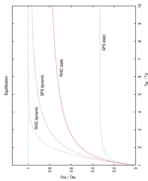
Figure 2: Degree of the chemical equilibrium reached for different break-up times $t_{{\rm br}}/t_{0}$ at initial inter-collison times $t_{c}/t_{0}=1/3$ for SPS (3-dimensional) and RHIC (1-dimensional) expansion scenarios with static and dynamic confinement (hadronization cross section is inversely proportional to the color density).

5 Conclusion

In conclusion 1) the results of the statistical model can be interpreted not only by assuming hadronic equilibrium, but as well by quark – hadron mixture chemistry with quarks eventually suppressed due to confinement. This interpretation avoids the collision time problem: the hadrons need not transmutate into each other directly. 2) The ALCOR and constrained hadronic equilibrium leads to the same result in the simple scenario presented here due to the constraints on conserved quantities. Quark coalescence, which takes conservation into account, closely mimics hadronic statistics in chemical equilibrium. This feature does not generalize for several competing reaction channels, but the overall picture is still similar. 3) $\gamma_{C}\approx 0.3$ is typical for spherical expansion (CERN SPS) without considering dynamical confinement, even for an arbitrary long hadronization process. The experimental evidence, reaching at least 70-80% of equilibrium ratios for almost all hadrons in a short time in the order of several fm/c, excludes this possibility. It also underlines the quark matter hadronization scenario with dynamical confinement effect, as transchemistry utilizes it. 4) A purely longitudinal expansion scenario, perhaps typical for RHIC and LHC energies, in principle allows for reaching the equilibrium even with static confinement only, but the process is rather slow and an early break-up may prevent some quarks from hadronizing. Dynamical confinement has to be in work for near one-dimensional expansion scenarios with a minor transverse flow, too. 5) We pointed out that total elimination of free quarks in an expanding quark matter scenario in the presence of any transverse flow requires a quark density dependence of the hadronization cross section, which is at least $1/n$. We call this effect “dynamical” confinement, it evidently cannot be of perturbative origin.

One is tempted to speculate about the dynamical confinement, looking for a cause of the density dependence of the hadronization cross section. Since this dependence makes the cross section stronger and even diverging with diminishing quark density, it cannot have perturbative origin. In our view it has to do with the formation of strings or color ropes, which become longer and hence more efficiently bind quarks into hadronic (color neutral) clusters as the color charge density drops.

Acknowledgements This work was supported by the US-Hungarian Joint Fund TéT 649 and by the Hungarian National Research Fund OTKA T029158.

References

- [1]
- [2] J. Rafelski and B. Müller, Phys. Rev. Lett. 48 (1982) 1066.
- [3] T. Biró and J. Zimányi, Phys. Lett. B113 (1982) 6.
- [4] P. Braun-Münzinger, I. Heppe and J. Stachel, Phys. Lett. B465 (1999) 15 [nucl-th/9903010].
- [5] F. Becattini, M. Gazdzicki and J. Sollfrank, Nucl. Phys. A638 (1998) 403.
- [6] J. Cleymans, H. Oeschler and K. Redlich, J. Phys. G G25 (1999) 281 [nucl-th/9809031].
- [7] J. Letessier and J. Rafelski, Phys. Rev. C59 (1999) 947 [hep-ph/9806386].
- [8] A. Bialas, Phys. Lett. B442 (1998) 449 [hep-ph/9808434].
- [9] T. S. Biró, P. Lévai and J. Zimányi, Phys. Lett. B347 (1995) 6.
- [10] T. S. Biró, P. Lévai and J. Zimányi, Phys. Rev. C59 (1999) 1574.
- [11] K. Geiger, Phys. Rev. D47 (1993) 133.
- [12] K. Geiger, Phys. Rev. D56 (1997) 2665 [hep-ph/9611400].
- [13] K. Werner, J. Hufner, M. Kutschera and O. Nachtmann, Z. Phys. C37 (1987) 57.
- [14] K. J. Eskola, B. Müller and X. Wang, Phys. Lett. B374 (1996) 20 [hep-ph/9509285].
- [15] H. Sorge, Phys. Lett. B344 (1995) 35.
- [16] J. Sollfrank, U. Heinz, H. Sorge and N. Xu, J. Phys. G25 (1999) 363 [nucl-th/9811011].
- [17] F. Antinori et al. [WA97 Collaboration], Eur. Phys. J. C11 (1999) 79.
- [18] M. Bleicher, S. A. Bass, H. Stöcker and W. Greiner, “RHIC predictions from the UrQMD model,” hep-ph/9906398.
- [19] N. S. Amelin and L. V. Bravina, Sov. J. Nucl. Phys. 51 (1990) 133.
- [20] D. J. Dean, M. Gyulassy, B. Müller, E. A. Remler, M. R. Strayer, A. S. Umar and J. S. Wu, Phys. Rev. C46 (1992) 2066.
- [21] S. A. Bass et al., Prog. Part. Nucl. Phys. 41 (1998) 225 [nucl-th/9803035].
- [22] C. T. Traxler, U. Mosel and T. S. Biró, Phys. Rev. C59 (1999) 1620 [hep-ph/9808298].
- [23] T. S. Biró, Phys. Lett. B143 (1984) 50.