Abstract

Starting from general considerations about the different concepts which exist for the definition of the quark mass near the pair production threshold, we introduce the definition of a mass with a dynamic degree of freedom that extends the previously given concept of the static PS mass.

Talk given by Stefan Groote at the Laboratory of Nuclear Studies,
Cornell University, Ithaca, NY, August 23rd, 2000

1 Keeping up with experiments

Besides existing machines and a whole bunch of data sets, further lepton pair colliders such as the Next Linear Collider (NLC) and the Future Muon Collider (FMC) are designed for the future. They will be able to determine the properties of heavy particles to an extend never reached by present colliders. Especially they will be able to measure the properties of the top quark which was first measured at the Tevatron with a mass of $m_{t}=174.3\pm 5{\,\rm GeV\/}$ (see e.g. [1] and references therein). Although the top quark will be studied at the LHC and the Tevatron (RUN-II) as well with an expected accuracy for the mass of $2-3{\,\rm GeV\/}$, the measurements at NLC are expected to have an accuracy of $0.1\%$ ($100-200{\,\rm MeV\/}$) [2].

Theorists are therefore asked to improve their predictions, too. Of special interest is the consideration of the cross section near the pair production threshold because the resonance observed there is constituted solely by a colour singlet state. A lot has been done in the past and just recently to calculate and match corresponding diagrams up to the next-to-next-to-leading order in order to determine this cross section (for an overview on work that has been done see e.g. Ref. [3]). But the question remains what we actually want to determine. What can we say about the mass of a particle which never will show up in nature in isolated fashion because of its confinement? Does the term of the mass of the top quark really makes sense?

The everydays life of theorists show that this actually makes no sense. There are different concepts on the market – each of them with different advantages and disadvantages, regions of validy and failure. They all show that there cannot be a unique definition of the quark mass. Instead the task of the theory can only be to quantify and limit the theoretical uncertainties to an amount comparable to the experimental measurements. One of these theory-born uncertainties are special kinds of IR singularities known as renormalons which limit the accuracy of a prediction to the order of $\Lambda_{\rm QCD}$. Just recently this problem has been overcome (a synapsis of the progress is given in Ref. [4]), and this talk will deal with the different concepts which were developed in this context, closing with an own suggestion presented by the authors [3].

2 $\overline{\rm MS}$ mass and on-shell or pole mass

A mass quite often used in perturbation theory is the $\overline{\rm MS}$ mass. It is related to the bare mass of the underlying QCD by the calculation of self energy diagrams of the quark. The term $\overline{\rm MS}$ mass indicates that for this calculation we use the $\overline{\rm MS}$ subtraction scheme which itself is based on the dimensional regularization method. The calculation of self energy diagrams which is done actually up to the third order QCD perturbation theory [5, 6] leads to a couple of master diagrams which are calculated at center-of-mass energies in the deep Euklidean domain ($q^{2}<0$, $|q|$ large) where the perturbation series converge sufficiently good. This $\overline{\rm MS}$ mass of course does not fit the range around the threshold and spoils the non-relativistic expansion if applied. But the $\overline{\rm MS}$ mass can be continued to this region.

The continuation is done by the Borel transformation. This transform can be understood as the extrapolation from the deep Euklidean domain to the $t\bar{t}$ threshold domain where a simultaneous limit of the negative center-of-mass energy and the order of the used derivative is taken. The ratio of these two quantities remains fixed and constitutes the Borel parameter. As shown in Ref. [7], this Borel transformation can be made explicit for the case of the “large $\beta_{0}$ limit” where the prescription of Brodsky, Lepage and Mackenzie [8] is used to sum up all fermion loop insertions (being proportional to the zeroth order QCD beta function coefficient $\beta_{0}=11C_{A}/3-2N_{F}/3$) in order to obtain an estimate (for a relation of this estimate to the $\overline{\rm MS}$ mass see Ref. [9]).

If we use the prescription for the static quark-antiquark potential $V(r)$, we obtain

$$V(r)=\sum_{n=0}^{\infty}V_{n}(\beta_{0}\alpha_{s})^{n+1}.$$ (1)

The Borel transformation of this series expression leads to

$$\tilde{V}(r;u)=\sum_{n=0}^{\infty}\frac{V_{n}}{n!}u^{n}$$ (2)

The series for the Borel transformed quantity converges even if the perturbative series for $V(r)$ itself is divergent. The inverse Borel transformation

$$V(r)=\int_{0}^{\infty}e^{u/(\beta_{0}\alpha_{s})}\tilde{V}(r;u)du$$ (3)

provides then a good definition. However, there might occur singularities on the integration contour. As mentioned before, for the “large $\beta_{0}$” estimate (also known as “naive non-abelianization”) we obtain an explicit expression

$$\tilde{V}(r;u)\sim\frac{\Gamma(1/2+u)\Gamma(1/2-u)}{\Gamma(2u+1)}$$ (4)

which has simple poles for $u=k+1/2$, $k=0,1,2,\ldots$. These singularities are a special case of IR renormalons.

The same happens then for the continuation of the $\overline{\rm MS}$ mass to the on-shell mass in the threshold region. This on-shell mass is appropriate to the treatment near the threshold because the quark is then assumed to be nearly on-shell. The on-shell mass $m$ (or pole mass as it is called more often) can be determined by the demand that the inverse Fermi propagator should vanish at this point,

$$(S_{F}(q))^{-1}\Big{|}_{q^{2}=m^{2}}=0.$$ (5)

But the continuation of the $\overline{\rm MS}$ mass via Borel transformation to the pole mass leads again to IR renormalon ambiguities.

So there is no way out? Wait, there is one! Both the pole mass and the static potential show an IR renormalon ambiguity. Maybe they cancel in a specific combination of these two quantities? Indeed it emerges that in the combination $2m+V(r)$ the IR sensitivity vanishes. Only for this reason it is then possible to construct a quantity which has no such ambiguities. In fact there are several of them, called threshold masses which we will deal with in the following.

3 Threshold mass definitions

The first definition we want to mention here is the definition given by Hoang and Teubner [10]. We mention it first because it is the most sophisticated definition. Starting with the non-relativistic QCD (NRQCD) [11], an effective theory designed to handle the non-relativistic quark-antiquark system which separates the low-momentum scales $mv$ and $mv^{2}$ from the high momentum scale $m$ ($v$ is the velocity of the quark), they stress the relevance of the different scales $v$ and $\alpha_{s}$ and their interrelation. Especially in the non-relativistic regime even the space and time components can be scaled differently. So there are “soft” ($q\sim m(v;v)$), “potential” ($q\sim m(v^{2};v)$), and “ultrasoft” regions ($q\sim m(v^{2};v^{2})$) where the last one is populated only by gluons, not by quarks. If we separate the dynamical degrees of freedom also from the “soft” heavy quarks and gluons and the “potential” gluons, supplemented by an expansion in momentum components to the order $mv^{2}$, this leads to the construction of the “potential NRQCD” (PNRQCD) [12] with the Langrangian

$${\cal L}_{\rm PNRQCD}=\tilde{\cal L}_{\rm NRQCD}+\int(\psi^{\dagger}\psi)(\vec{r}\,)V(\vec{r}\,)(\chi^{\dagger}\chi)(\vec{0})d^{3}r.$$ (6)

Here the heavy quark-antiquark potential $V(\vec{r}\,)$ occurs, $\psi$ and $\chi$ are the quark and antiquark spinors, respectively. Finally the authors of Ref. [10] come to the conclusion that an adequate threshold mass definition is given by one half of the perturbative mass of a fictious toponium $1^{3}S_{1}$ ground state. This threshold mass definition is referred to in the literature as $1S$ mass.

A second threshold mass definition is given by Bigi et al. [13] and is known by the name “low scale” (LS) mass.

Finally, Beneke gave a definition which then led to the generalization suggested by us. The static potential subtracted (PS) mass [14] is the minimal version of a threshold mass. As the name tells us, the definition is given by combining IR singular parts taken from the static quark-antiquark potential with the pole mass in order to cancel out the IR sensitivity. Starting point is the observation that the IR sensitive parts of the potential stem from long distance contributions, i.e. small values of the three-momentum. If we therefore restrict the three-momentum range of the potential as expressed by the Fourier transformation

$$V(|\vec{r}\,|)=\int\frac{d^{3}q}{(2\pi)^{3}}e^{i\vec{q}\cdot\vec{r}}\tilde{V}(|\vec{q}\,|)$$ (7)

by $|\vec{q}\,|<\Lambda_{\rm QCD}$, this results (for the leading order Coulomb potential) in the contribution

$$\int_{|\vec{q}\,|<\Lambda_{\rm QCD}}\frac{d^{3}q}{(2\pi)^{3}}e^{i\vec{q}\cdot\vec{r}}\left(-\frac{4\pi\alpha_{s}C_{F}}{\vec{q}\,^{2}}\right)=-\frac{2\alpha_{s}C_{F}}{\pi}\Lambda_{\rm QCD}+O(\Lambda_{\rm QCD}^{3}r^{2})$$ (8)

which restricts the accuracy. The way out is to use a potential $V(r;\mu_{f})$ defined by the Fourier transformation with $|\vec{q}\,|>\mu_{f}$ and to subsume the remaining part to the mass,

$$m_{\rm PS}(\mu_{f})=m-\delta m_{\rm PS}(\mu_{f}),\qquad\delta m_{\rm PS}(\mu_{f})=-\frac{1}{2}\int_{|\vec{q}\,|<\mu_{f}}\frac{d^{3}q}{(2\pi)^{3}}\tilde{V}(|\vec{q}\,|)$$ (9)

(it is legitimate to use $e^{i\vec{q}\cdot\vec{r}}\approx 1$ here). The scale $\mu_{f}$ introduced by this is called factorization scale. It drops out again if the static PS mass is related to the $\overline{\rm MS}$ mass.

4 A dynamic mass definition

It has been pointed out already in Ref. [14] that the replacement

$$\frac{1}{v\cdot q}\rightarrow-i\pi\delta(v\cdot q)$$ (10)

in the self energy leads to the leading infrared behaviour. We have taken this consideration as starting point for our definition and extended it to the more general non-static case.

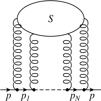
Figure 1: The general structure of the self energy diagram of a quark

The general structure of the self energy diagram for an on-shell quark with mass $m$ and momentum $p$ ($p^{2}=m^{2}$) is shown in Fig. 1. The expression for this diagram is given by

$$-i\Sigma(p\kern-5.0pt/) = \int\prod_{m=1}^{M}\frac{d^{4}l_{m}}{(2\pi)^{4}}S^{\{a_{n}\}}_{\{\alpha_{n}\}}(\{l_{m}\})\left(-ig_{s}\gamma^{\alpha_{N+1}}T_{a_{N+1}}\right)\ \times$$ (11)

$$\qquad\qquad\qquad\times\ \prod_{n=N}^{1}\frac{i}{p\kern-5.0pt/_{n}-m}\left(-ig_{s}\gamma^{\alpha_{n}}T_{a_{n}}\right)$$

where the last factor is a non-commutative product with decreasing index $n$. The line momenta $k_{n}$ are linear combinations of the gluon loop momenta $l_{m}$, the particular representation is specified by the structure $S$. The symbol $\{l_{m}\}$ means the set of all these loop momenta, the same symbol is used for the Lorentz and colour indices. In general we have $M\leq N$ which means that line momenta can be correlated. The momenta of the virtual quark states are given by $p_{n}=p+k_{n}$.

The quark is considered to be at rest, $p=(m,\vec{0})$, and it interacts with a number of gluons. The subdiagram $S$ displayed in Fig. 1 describes the interaction between the gluons. In general the quark lines between the interaction points represent virtual quark states. However, if the virtual quark comes very close to the mass shell and the total momentum of the cloud of virtual gluons becomes soft, this situation gives rise to long-distance nonperturbative QCD interactions. The described (virtual) contributions results in the soft part of the self energy, $\Sigma_{\rm soft}$. So we define

$$-i\Sigma_{\rm soft}(p\kern-5.0pt/)\ =\ \sum_{i=1}^{N}\int\prod_{m=1}^{M}\frac{d^{4}l_{m}}{(2\pi)^{4}}S^{\{a_{n}\}}_{\{\alpha_{n}\}}(\{l_{m}\})\left(-ig_{s}\gamma^{\alpha_{N+1}}T_{a_{N+1}}\right)\ \times$$ (12)

$$\times\ \prod_{n=N}^{i+1}\frac{i}{p\kern-5.0pt/_{n}-m}\left(-ig_{s}\gamma^{\alpha_{n}}T_{a_{n}}\right)i(p\kern-5.0pt/_{i}+m)\left(-i\pi\delta(p_{i}^{2}-m^{2})\right)\ \times$$

$$\qquad\times\ \left(-ig_{s}\gamma^{\alpha_{i}}T_{a_{i}}\right)\prod_{n=i-1}^{1}\frac{i}{p\kern-5.0pt/_{n}-m}\left(-ig_{s}\gamma^{\alpha_{n}}T_{a_{n}}\right).$$

One can derive this expression from Eq. (11) by using the identity

$$\frac{1}{p^{2}-m^{2}+i\epsilon}=-i\pi\delta(p^{2}-m^{2})+P\left(\frac{1}{p^{2}-m^{2}}\right)$$ (13)

and the fact that the principal value integral does not give any infrared sensitive contribution. The delta function can be used to remove the integration over the zero component of $k_{i}$. In order to parameterize the softness of the gluon cloud we impose a cutoff on the spatial component, $|\vec{k}_{i}|<\mu_{f}$, and indicate this by the label $\mu_{f}$ for the factorization scale written at the upper limit of the three-dimensional integral. So we can rewrite Eq. (12) as

$$\Sigma_{\rm soft}(p\kern-5.0pt/,\mu_{f})=-\frac{1}{2}\sum_{i=1}^{N}\int^{\mu_{f}}\frac{d^{3}k_{i}}{(2\pi)^{3}}V(\vec{k}_{i},p)$$ (14)

where

$$V(\vec{k}_{i},p)\ =\ -\int\prod_{m=1}^{M-1}\frac{d^{4}l_{m}}{(2\pi)^{4}}S^{\{a_{n}\}}_{\{\alpha_{n}\}}(\{l_{m}\})\left(-ig_{s}\gamma^{\alpha_{N+1}}T_{a_{N+1}}\right)\ \times$$

$$\kern-24.0pt\times\ \prod_{n=N}^{i+1}\frac{i}{p\kern-5.0pt/_{n}-m}\left(-ig_{s}\gamma^{\alpha_{n}}T_{a_{n}}\right)\frac{p\kern-5.0pt/_{i}+m}{2p_{i}^{0}}\left(-ig_{s}\gamma^{\alpha_{i}}T_{a_{i}}\right)\prod_{n=i-1}^{1}\frac{i}{p\kern-5.0pt/_{n}-m}\left(-ig_{s}\gamma^{\alpha_{n}}T_{a_{n}}\right)$$

and finally define

$$m_{\overline{\rm PS}}=m-\delta m_{\overline{\rm PS}}\quad\mbox{with}\quad\delta m_{\overline{\rm PS}}=\Sigma_{\rm soft}(p\kern-5.0pt/)\Big{|}_{p\kern-5.0pt/=m}.$$ (16)

In the following we deal with the different realizations of this compact expression. As we will see explicitly, the function $V(\vec{k},p)$ occurring as integrand can be seen as quark-antiquark potential where we have summed over the spin of the tensor product of a final state with an initial state. Because the static quark-antiquark potential is used in a similar way in Ref. [14], we recover the result of Ref. [14] in the static limit.

5 The one-loop contribution

The leading order contribution to the self energy of the quark is given by

$$\Sigma(p\kern-5.0pt/)=i\int\frac{d^{4}k}{(2\pi)^{4}}(-ig_{s}\gamma_{\alpha}T_{a})\frac{i}{p\kern-5.0pt/+/\kern-6.0ptk-m}(-ig_{s}\gamma^{\alpha}T_{a})\frac{-i}{k^{2}}$$ (17)

where Feynman gauge is used for the gluon. The soft part of it is given by

$$\Sigma_{\rm soft}(p\kern-5.0pt/,\mu_{f})=-\frac{1}{2}\int^{\mu_{f}}\frac{d^{3}k}{(2\pi)^{3}}V(\vec{k},p),\qquad V(\vec{k},p)=V_{+}(\vec{k},p)+V_{-}(\vec{k},p)$$ (18)

where

$$V_{\pm}(\vec{k},p)=-\frac{g_{s}^{2}C_{F}(\sqrt{m^{2}+\kappa^{2}}\mp 2m)}{2m\sqrt{m^{2}+\kappa^{2}}(\sqrt{m^{2}+\kappa^{2}}-m)}$$ (19)

and $\kappa=|\vec{k}|$. The procedure of taking the soft part by setting a cut is shown in Fig. 2(a–b).

Figure 2: Leading order contribution to the quark self energy (a) and to the quark-antiquark potential (b). The cross indicates the point where we cut the quark line by imposing an on-shell condition to the virtual quark state. In Coulomb gauge the gluon propagator can be decomposed in a Coulomb propagator (c) and a transverse propagator (d).

The two potential parts are known as the scattering potential $V_{+}(\vec{k},p)$ and the annihilation potential $V_{-}(\vec{k},p)$ and correspond to the two zeros $k_{\pm}=\pm\sqrt{\kappa^{2}+m^{2}}-m$ of the delta function. Integrating the potential up to the factorization scale $\mu_{f}$, we obtain

$$\Sigma_{\rm soft}(\mu_{f})=\frac{\alpha_{s}C_{F}}{2\pi}m\left\{3\ln\left(\frac{\mu_{f}}{m}+\sqrt{\frac{\mu_{f}^{2}}{m^{2}}+1}\,\right)-\frac{\mu_{f}}{m}\sqrt{\frac{\mu_{f}^{2}}{m^{2}}+1}\,\right\}.$$ (20)

The expansion of this expression in small values of $\mu_{f}/m$ results in

$$\Sigma_{\rm soft}(\mu_{f})=\frac{\alpha_{s}C_{F}}{\pi}\mu_{f}\left\{1-\frac{\mu_{f}^{2}}{2m^{2}}+O\left(\frac{\mu_{f}^{4}}{m^{4}}\right)\right\}.$$ (21)

The first term reproduces the result given in Ref. [14] to leading order in $\alpha_{s}$ while the second term is the recoil correction to the static limit in this order of perturbation theory. This second term is related to the Breit-Fermi potential but does not coincide with it.

6 Two-loop contributions

To take a step beyond the leading order perturbation theory, we consider two-loop diagrams for the heavy quark self energy as shown in Fig. 3.

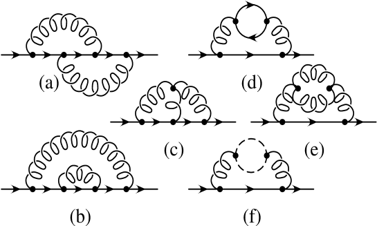
Figure 3: Two-loop contributions to the quark self energy

In cutting the quark line in all possible ways we obtain a lot of diagrams from the ones shown in Fig. 3. However, we find that the final contribution of the two abelian diagrams in Fig. 3(a–b) to the soft part of the self energy is suppressed by $\mu_{f}^{2}/m^{2}$. Therefore it turns out that the only abelian diagrams which can give a non-suppressed contribution to the soft part of the quark self energy are the diagrams containing the vacuum polarization of the gluon as shown in Fig. 3(d–f). The simple calculation of these diagrams within the $\overline{\rm MS}$ scheme, accounting only for light fermion loops, gluon loop (and ghost loop if Feynman gauge is used) results after renormalization in

$$\Sigma_{\rm soft}^{A} = -\frac{1}{2}\int^{\mu}\frac{d^{3}k}{(2\pi)^{3}}\left(-\frac{4\pi\alpha_{s}(\mu)C_{F}}{|\vec{k}|^{2}}\right)\left\{1+\frac{\alpha_{s}(\mu)}{4\pi}\left(a_{1}-\beta_{0}\ln\left(\frac{|\vec{k}|^{2}}{\mu^{2}}\right)\right)\right\}$$ (22)

$$= \frac{\alpha_{s}(\mu)C_{F}}{\pi}\mu_{f}\left\{1+\frac{\alpha_{s}(\mu)}{4\pi}\left(a_{1}-\beta_{0}\ln\left(\frac{\mu_{f}^{2}}{\mu^{2}}\right)\right)\right\}$$

with the same coefficient $a_{1}$ as in Ref. [17] (see below). This result has been anticipated because the expression in the curly brackets of the integrand reproduces the next-to-leading order correction to the QCD Coulomb potential.

For the only non-abelian diagram in Fig. 3(c) we obtain

$$\Sigma_{\rm soft}^{NA}=\frac{\alpha_{s}^{2}C_{F}C_{A}}{8m}\mu_{f}^{2}.$$ (23)

This result has been anticipated, too, to be minus one half of the non-abelian correction to the QCD Coulomb potential, which is known in the literature (see for example Refs. [15, 16]),

$$\Sigma_{\rm soft}^{NA} = -\frac{1}{2}\int^{\mu_{f}}\frac{d^{3}k}{(2\pi)^{3}}\left\{-\frac{\pi^{2}\alpha_{s}^{2}C_{F}C_{A}}{m|\vec{k}|}\right\}\ =\ \frac{\alpha_{s}^{2}C_{F}C_{A}}{8m}\mu_{f}^{2}.$$ (24)

7 Our final result

Summarizing all contribution up to NNLO accuracy, we obtain

$$m_{\overline{\rm PS}}(\mu_{f})-m = -\frac{\alpha_{s}(\mu)C_{F}}{\pi}\mu_{f}\Bigg{\{}1+C^{\prime}_{0}\frac{\mu_{f}}{m}+C^{\prime\prime}_{0}\frac{\mu_{f}^{2}}{m^{2}}\,+$$ (25)

$$\qquad+\frac{\alpha_{s}(\mu)}{4\pi}\left(C_{1}+C^{\prime}_{1}\frac{\mu_{f}}{m}\right)+C_{2}\left(\frac{\alpha_{s}(\mu)}{4\pi}\right)^{2}\Bigg{\}}$$

(a result to a not yet specified order in $\mu_{f}/m$) where $m$ is the pole mass, $\mu$ is the renormalization scale, $\mu_{f}$ is the factorization scale, and

$$C_{0} = 1,\qquad C^{\prime}_{0}\ =\ 0,\qquad C^{\prime\prime}_{0}\ =\ -\frac{1}{2},$$

$$C_{1} = a_{1}-2\beta_{0}\ln\left(\frac{\mu_{f}}{\mu}\right),\qquad C^{\prime}_{1}\ =\ C_{A}\frac{\pi^{2}}{2},$$

$$C_{2} = a_{2}-2(2a_{1}\beta_{0}+\beta_{1})\left(\ln\left(\frac{\mu_{f}}{\mu}\right)-1\right)\,+$$ (26)

$$\qquad+4\beta_{0}^{2}\left(\ln^{2}\left(\frac{\mu_{f}}{\mu}\right)-2\ln\left(\frac{\mu_{f}}{\mu}\right)+2\right).$$

The constants $a_{1}$ and $a_{2}$ are given by [17, 18, 19]

$$a_{1} = \frac{31}{9}C_{A}-\frac{20}{9}T_{F}N_{F},$$

$$a_{2} = \left(\frac{4343}{162}+4\pi^{2}-\frac{\pi^{4}}{4}+\frac{22}{3}\zeta_{3}\right)C_{A}^{2}-\left(\frac{1798}{81}+\frac{56}{3}\zeta_{3}\right)C_{A}T_{F}N_{F}\,+$$ (27)

$$+\left(\frac{20}{9}T_{F}N_{F}\right)^{2}-\left(\frac{55}{3}-16\zeta_{3}\right)C_{F}T_{F}N_{F},$$

the coefficients of the beta function are known as

$$\beta_{0}=\frac{11}{3}C_{A}-\frac{4}{3}T_{F}N_{F},\quad\beta_{1}=\frac{34}{3}C_{A}^{2}-\frac{20}{3}C_{A}T_{F}N_{F}-4C_{F}T_{F}N_{F}$$ (28)

where $C_{F}=4/3$, $C_{A}=3$ and $T_{F}=1/2$ are colour factors and $N_{F}=5$ is the number of light flavours. The coefficients $C_{1}$ and $C_{2}$ in Eq. (25) have been derived in Ref. [14] by using known corrections to the QCD potential. In Ref. [3] we have obtained the coefficients $C^{\prime}_{0}$, $C^{\prime\prime}_{0}$, and $C^{\prime}_{1}$. Note that our result can be represented in a condensed form as

$$m_{\overline{\rm PS}}(\mu_{f})-m=-\frac{1}{2}\int^{\mu_{f}}\frac{d^{3}k}{(2\pi)^{3}}\left(V_{C}(|\vec{k}|)+V_{R}(|\vec{k}|)+V_{NA}(|\vec{k}|)\right)$$ (29)

where the first term $V_{C}$ is the static Coulomb potential, $V_{R}$ is the relativistic correction (which is related to Breit-Fermi potential but does not coincide with it), and $V_{NA}$ is the non-abelian correction. Note that we did not include electroweak corrections in our calculations.

$\overline{m}(\overline{m})$	$m_{\rm PS}^{\rm LO}$	$m_{\rm PS}^{\rm NLO}$	$\displaystyle\matrix{m_{\rm PS}^{\rm NNLO}\cr m_{\overline{\rm PS}}^{\rm NNLO}}$	$m_{\rm pole}^{\rm LO}$	$m_{\rm pole}^{\rm NLO}$	$m_{\rm pole}^{\rm NNLO}$
160	166.51	167.69	$\displaystyle\matrix{167.97\cr 167.95}$	167.44	169.05	169.56
165	171.72	172.93	$\displaystyle\matrix{173.22\cr 173.20}$	172.64	174.28	174.80
170	176.92	178.17	$\displaystyle\matrix{178.47\cr 178.45}$	177.84	179.52	180.05

Table 1: Top quark mass relations for the $\overline{\rm MS}$, PS, $\overline{\rm PS}$, and the pole mass at LO, NLO, and NNLO in ${\,\rm GeV\/}$. We fix the $\overline{\rm MS}$ mass to be $\overline{m}(\overline{m})=160{\,\rm GeV\/}$, $165{\,\rm GeV\/}$, and $170{\,\rm GeV\/}$ and find the pole mass at LO, NLO, and NNLO from the three-loop relation in Refs. [5, 6]. The PS and $\overline{\rm PS}$ masses are derived from the pole mass by using Eq. (25) (without or with the $1/m$ contributions, respectively). We use the QCD coupling constant $\alpha_{s}(m_{Z})=0.119$ [20], $\mu=\overline{m}(\overline{m})$, and $\mu_{f}=20{\,\rm GeV\/}$.

Using the relation given by Eq. (25) between $m_{\overline{\rm PS}}$ and $m$ as well as the relation between $m$ and $\overline{m}(\overline{m})$ given in Refs. [5, 6], we fix the $\overline{\rm MS}$ mass to take the values $\overline{m}(\overline{m})=160{\,\rm GeV\/}$, $165{\,\rm GeV\/}$, and $170{\,\rm GeV\/}$ and determine the pole mass at LO, NLO, and NNLO. This pole mass is then used as input parameter $m$ in Eq. (25) to determine the PS and $\overline{\rm PS}$ masses at LO, NLO, and NNLO. The results of these calculations are collected in Table 1. Taking the $\overline{\rm PS}$ mass instead of the PS mass, we observe an improvement of the convergence. The differences for the mass values in going from LO to NLO to NNLO for e.g. $\overline{m}(\overline{m})=165{\,\rm GeV\/}$ read $7.64{\,\rm GeV\/}$, $1.64{\,\rm GeV\/}$, and $0.52{\,\rm GeV\/}$ for the pole mass, $6.72{\,\rm GeV\/}$, $1.21{\,\rm GeV\/}$, and $0.29{\,\rm GeV\/}$ for the PS mass and finally $6.72{\,\rm GeV\/}$, $1.21{\,\rm GeV\/}$, and $0.27{\,\rm GeV\/}$ for the $\overline{\rm PS}$ mass. So the tendency is going in the proper direction. However, we stress that the goal, namely to avoid the infrared renormalon ambiguities, is already reached by the static PS mass as well as by the other threshold masses which have been developed.

8 What to do with our result then?

Having mass values for the top quark at hand, we can consider the cross section of the process $e^{+}e^{-}\to t\bar{t}$ in the near threshold region where the velocity $v$ of the top quark is small. It is well known that the conventional perturbative expansion does not work in the non-relativistic region because of the presence of the Coulomb singularities at small velocities $v\to 0$. The terms proportional to $(\alpha_{s}/v)^{n}$ appear due to the instantaneous Coulomb interaction between the top and the antitop quark. The standard technique for resumming the terms $(\alpha_{s}/v)^{n}$ consists in using the Schrödinger equation for the quark-antiquark potential [21]

$$(H-E-i\Gamma)G(\vec{r},\vec{r}\,^{\prime}|E+i\Gamma)=\delta^{3}(r-r^{\prime})$$ (30)

where $H$ is the non-relativistic Hamiltonian of the heavy quark-antiquark system, to find the Green function. The Green function is then related to the relative cross section by the optical theorem,

$$R = \frac{\sigma(e^{+}e^{-}\to t\bar{t})}{\sigma(e^{+}e^{-}\to\mu^{+}\mu^{-})}\ =$$ (31)

$$= e^{2}_{Q}N_{c}\frac{24\pi}{s}C(r_{0}){\rm Im}\left[\left(1-\frac{\vec{p}\,^{2}}{3m^{2}}\right)G(r_{0},r_{0}|E+i\Gamma)\right]\Bigg{|}_{r_{0}\to 0}$$

where $\sigma(e^{+}e^{-}\to\mu^{+}\mu^{-})=4\pi\alpha^{2}/3s$, $e_{Q}$ is the electric charge of the top quark, $N_{c}$ is the number of colours, $\sqrt{s}=2m+E$ is the total center-of-mass energy of the quark-antiquark system, $m$ is the top quark pole mass and $\Gamma$ is the top quark width. The unknown short distance coefficient $C(r_{0})$ can be fixed by using a direct QCD calculation of the vector vertex at NNLO in the so-called intermediate region [22, 23] and by using the direct matching procedure suggested in Ref. [24].

If we take the PS mass as input parameter instead of the pole mass, the energy value $E$ has to be changed to $\sqrt{s}-2m_{\rm PS}(\mu_{f})$ instead of $\sqrt{s}-2m$. The same holds for the $\overline{\rm PS}$ mass. It is shown [10, 25, 26] that the Schrödinger equation can be reduced to the equation

$$(H_{1}-E_{1})G_{1}(r,r^{\prime}|E_{1})=\delta^{3}(r-r^{\prime})$$ (32)

with the energy $E_{1}=\bar{E}+\bar{E}^{2}/4m$, $\bar{E}=E+i\Gamma$, and with the Hamiltonian

$$H_{1} = \frac{\vec{p}\,^{2}}{m}+V_{C}(r)+\frac{3\bar{E}}{2m}V_{0}(r)-\left(\frac{2}{3}+\frac{C_{A}}{C_{F}}\right)\frac{V_{0}^{2}(r)}{2m},$$

$$V_{0}(r) = -\frac{\alpha_{s}(\mu)C_{F}}{r},$$

$$V_{C}(r) = V_{0}(r)\Bigg{\{}1+\frac{\alpha_{s}(\mu)C_{F}}{4\pi}\left(2\beta_{0}\ln(\mu^{\prime}r)+a_{1}\right)\,+$$

$$\kern-24.0pt+\left(\frac{\alpha_{s}(\mu)}{4\pi}\right)^{2}\left(\beta_{0}^{2}\left(4\ln^{2}(\mu^{\prime}r)+\frac{\pi^{2}}{3}\right)+2(\beta_{1}+2\beta_{0}a_{1})\ln(\mu^{\prime}r)+a_{2}\right)\Bigg{\}}$$

where $\mu^{\prime}=\mu e^{\gamma_{E}}$, $\mu$ is the renormalization scale, and $\gamma_{E}$ is Euler’s constant. The final expression for the cross section is then given by

$$R=\frac{8\pi}{m^{2}}C(r_{0}){\rm Im}\left[\left(1-\frac{5\bar{E}}{6m}\right)G_{1}(r_{0},r_{0}|E_{1})\right]\Bigg{|}_{r_{0}\rightarrow 0}$$ (34)

with $G_{1}(r_{0},r_{0}|E_{1})$ being the solution of Eq. (32) at $r=r^{\prime}=r_{0}$. For the numerical solution we use the program derived in Ref. [26]. Note that we do not take into account an initial photon radiation which would change the shape of the cross section. This can be easily included in the Monte Carlo simulation.

Taking the pole mass as input parameter, the top quark cross section at LO, NLO, and NNLO is shown in Fig. 4 as a function of the center-of-mass energy. For the top quark pole mass we use $m_{t}=175.05{\,\rm GeV\/}$, for the top quark width $\Gamma_{t}=1.43{\,\rm GeV\/}$, and for the QCD coupling constant $\alpha_{s}(m_{Z})=0.119$ [20]. Different values $\mu=15{\,\rm GeV\/}$, $30{\,\rm GeV\/}$, and $60{\,\rm GeV\/}$ for the renormalization scale are selected because they roughly correspond to the typical spatial momenta for the top quark. We see that the NNLO curve modifies the line shape by the amount of $20-30\%$ which is as large as the NLO correction. It also shifts the position of the $1S$ peak by approximately $600{\,\rm MeV\/}$. These large shifts of the peak position are expected because of the renormalon ambiguity.

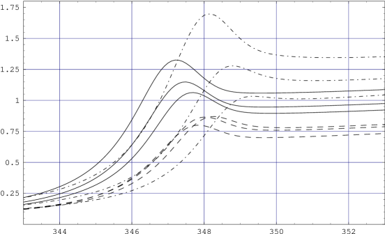
Figure 4: The scheme using the pole mass: shown is the relative cross section $R(e^{+}e^{-}\to t\bar{t})$ as a function of the center-of-mass energy in ${\,\rm GeV\/}$ for the LO (dashed-dotted lines), NLO (dashed lines), and NNLO (solid lines) approximation. We take the value $m_{t}=175.05{\,\rm GeV\/}$ for the pole mass of the top quark, $\Gamma_{t}=1.43{\,\rm GeV\/}$ for the top quark width, $\alpha_{s}(m_{Z})=0.119$ and different values $\mu=15{\,\rm GeV\/}$, $30{\,\rm GeV\/}$, and $60{\,\rm GeV\/}$ for the renormalization scale.

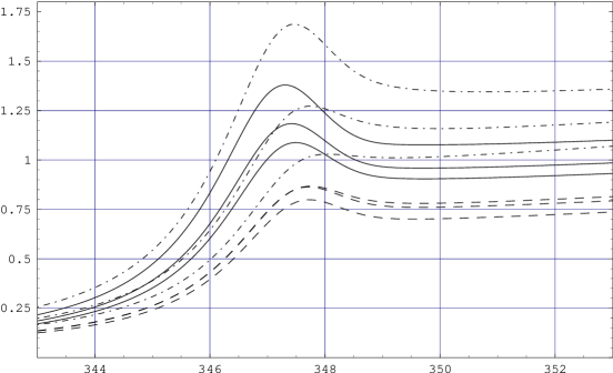
Figure 5: The scheme using the PS mass: shown is the relative cross section $R(e^{+}e^{-}\to t\bar{t})$ as a function of the center-of-mass energy in ${\,\rm GeV\/}$ for the LO (dashed-dotted lines), NLO (dashed lines), and NNLO (solid lines) approximation. We take the value $m_{\rm PS}=173.30{\,\rm GeV\/}$ for the PS mass of the top quark, $\Gamma_{t}=1.43{\,\rm GeV\/}$ for the top quark width, $\alpha_{s}(m_{Z})=0.119$ and different values $\mu=15{\,\rm GeV\/}$, $30{\,\rm GeV\/}$, and $60{\,\rm GeV\/}$ for the renormalization scale.

If we do the same for the PS mass value $m_{\rm PS}(\mu_{f}=20{\,\rm GeV\/})=173.30{\,\rm GeV\/}$ which corresponds to the pole mass $m=175.05{\,\rm GeV\/}$ according to the “large $\beta_{0}$” accuracy estimate, we obtain a picture like in Fig. 5 where we observe an improvement in the stability of the position of the first peak in comparison to the previous analysis as we go from LO to NLO to NNLO. Actually, for the three values $\mu=15{\,\rm GeV\/}$, $30{\,\rm GeV\/}$, and $60{\,\rm GeV\/}$ we obtain the maxima of the $1S$ peak for NNLO at $s_{\rm max}=347.32{\,\rm GeV\/}$, $347.41{\,\rm GeV\/}$, and $347.48{\,\rm GeV\/}$ while the maximal values are given by $R_{\rm max}=1.379$, $1.184$, and $1.088$, respectively. This demonstrated that a large variation in the renormalization scale $\mu$ gives rise only to a shift of about $160{\,\rm MeV\/}$ for the $1S$ peak position at NNLO while the variation for $R_{\rm max}$ is still large. The same procedure done for the $\overline{\rm PS}$ mass shows no observable difference. The differences shown in Table 1 are too small to make any viewable effect.

Conclusion and discussion

We discussed the potential subtracted (PS) mass suggested in Ref. [14] as a definition of the quark mass alternative to the pole mass. In contrast to the pole mass, this mass is not sensitive to the non-perturbative QCD effects. We have derived recoil corrections to the relation of the pole mass with the PS mass. In addition, we demonstrated that, if we use the PS or the $\overline{\rm PS}$ mass in the calculations, the perturbative predictions for the cross section become much more stable at higher orders of QCD (shifts are below $0.1{\,\rm GeV\/}$). This understanding removes one of the obstacles for an accurate top mass measurement and one can expect that the top quark mass will be extracted from a threshold scan at NLC with an accuracy of about $100-200{\,\rm MeV\/}$.
Acknowledgements: We are grateful to Ratindranath Akhoury, Ed Yao, Martin Beneke and Andre Hoang for valuable discussions. O.Y. acknowledges support from the US Department of Energy (DOE). S.G. acknowledges a grant given by the DFG, FRG, he also would like to thank the members of the theory group at the Newman Lab for their hospitality during his stay.

References

-
[1]
G. Brooijmans [CDF and D0 Collaborations],
“Top quark mass measurements at the Tevatron” [hep-ex/0005030] - [2] M.E. Peskin, “Physics goals of the linear collider” [hep-ph/9910521]
- [3] Oleg Yakovlev and Stefan Groote, “Top quark mass definition and production near threshold at the NLC” [hep-ph/0008156]
- [4] A.H. Hoang et al., Eur. Phys. J. direct C3 (2000) 1 [hep-ph/0001286]
-
[5]
K.G. Chetyrkin and M. Steinhauser,
Phys. Rev. Lett. 83 (1999) 4001 [hep-ph/9907509];
Nucl. Phys. B573 (2000) 617 [hep-ph/9911434] -
[6]
Kirill Melnikov and Timo van Ritbergen,
Phys. Lett. 482 B (2000) 99 [hep-ph/9912391] - [7] U. Aglietti and Z. Ligeti, Phys. Lett. 364 B (1995) 75 [hep-ph/9503209]
-
[8]
S.J. Brodsky, G.P. Lepage and P.B. Mackanzie,
Phys. Rev. D28 (1983) 288 -
[9]
M. Beneke and V.M. Braun,
Phys. Lett. 348 B (1995) 513 [hep-ph/9411229] -
[10]
A.H. Hoang and T. Teubner,
Phys. Rev. D60 (1999) 114027 [hep-ph/9904468] -
[11]
W.E. Caswell and G.P. Lepage,
Phys. Lett. 167 B (1986) 437;
G.T. Bodwin, E. Braaten and G.P. Lepage,
Phys. Rev. D51 (1995) 1125 [hep-ph/9407339] - [12] A. Pineda and J. Soto, Phys. Rev. D59 (1999) 016005 [hep-ph/9805424]
-
[13]
I.I. Bigi, M.A. Shifman, N.G. Uraltsev and A.I. Vainshtein,
Phys. Rev. D50 (1994) 2234 [hep-ph/9402360] - [14] M. Beneke, Phys. Lett. 434 B (1998) 115 [hep-ph/9804241]
-
[15]
S.N. Gupta and F. Radford,
Phys. Rev. D24 (1981) 2309; D25 (1982) 3430;
S.N. Gupta, F. Radford and W.W. Repko, Phys. Rev. D26 (1982) 3305 - [16] A. Duncan, Phys. Rev. D13 (1973) 2866
- [17] W. Fischler, Nucl. Phys. B129 (1977) 157
- [18] M. Peter, Nucl. Phys. B501 (1997) 471 [hep-ph/9702245]
- [19] Y. Schröder, Phys. Lett. 447 B (1999) 321 [hep-ph/9812205]
- [20] Particle Data Group (C. Caso et al.), Eur. Phys. J. C3 (1998) 1
-
[21]
V.S. Fadin and V.A. Khoze,
JETP Lett. 46 (1987) 525;
V.S. Fadin and V.A. Khoze, Sov. J. Nucl. Phys. 48 (1988) 309 -
[22]
A. Czarnecki and K. Melnikov,
Phys. Rev. Lett. 80 (1998) 2531 [hep-ph/9712222] -
[23]
M. Beneke and V.A. Smirnov,
Nucl. Phys. B522 (1998) 321 [hep-ph/9711391];
M. Beneke, A. Signer and V.A. Smirnov,
Phys. Rev. Lett. 80 (1998) 2535 [hep-ph/9712302] -
[24]
A.H. Hoang,
Phys. Rev. D56 (1997) 5851 [hep-ph/9704325];
Phys. Rev. D57 (1998) 1615 [hep-ph/9702331] -
[25]
K. Melnikov and A. Yelkhovsky,
Nucl. Phys. B528 (1998) 59 [hep-ph/9802379] - [26] O. Yakovlev, Phys. Lett. 457 B (1999) 170 [hep-ph/9808463]