B-physics phenomenology with emphasis on the light-cone

Abstract

Theoretical overviews on the B-physics are presented with an emphasis on the light-cone degrees of freedom. Our new treatment of the embedded states seems to give an encouraging result.

1 Introduction

With the wealth of new and upgraded experimental facilities for the B-physics, the precision test of standard model is ever more promising. The new facilities of BaBar at SLAC and Belle at KEK generate asymmetric $e^{+}e^{-}$ collisions to trace the B-decays more accurately. The symmetric $e^{+}e^{-}$ collision facility of CLEO-III at Cornell has also upgraded its luminosity by a factor of ten better. Furthermore, the hadon-hadron collision facilities such as LHCB at CERN and BTeV at Fermilab as well as the lepton-hadron collision facility such as HERA-B at DESY emerge as the powerful tools to investigate a lot of detailed B-decays [1]. Certainly, an important motivation to study B-physics is to make a precision test of standard model especially associated with the unitarity of CKM mixing matrix. One of the burning questions in physics is whether the complex phase is really the only source of the CP-violation or not. To make such a precision test, the accurate analyses of exclusive semileptonic B-decays as well as rare B-decays are strongly demanded. As we will discuss in this talk, an effective use of light-cone (LC) degrees of freedom in those analyses seem crucial to make the calculations more accurate. This also makes the model-building more scrutinized. Our talk is presented with the following outlines. The theoretical overview of B-physics is given in the next Section, Section 2. Especially, we will discuss the processes determining each CKM-matrix element and the profile of unitary triangle. We’ll also try to make a very brief survey of theoretical development in the last twenty years history of B-physics. Because of enormous works that people have done in B-physics, this survey would be in no way complete but very brief and limited. In any case, the purpose of Section 2 will be to motivate why the exclusive semileptonic B-decays are very important to constrain the CKM mixing matrix. In Section 3, then exclusive semileptonic decays are discussed. Some general remarks on the weak form factors will be made and the role of LC degrees of freedom in the exclusive semileptonic decays will be discussed. Especially, the difficulties associated with the time-like processes such as the exclusive semileptonic decays in the LC formulation. We will first identify the embedded states necessary to restore the covariance of the amplitudes and then present a way of handling the embedded states. Some preliminary numerical results are also presented in the exclusive semileptonic decays for $K\to\pi\ell\nu$ with our new way of treating the embedded states. Conclusions follow in Section 4.

2 The Theoretical Overview of B-Physics

In the standard model, the only interaction relevant to the CKM mixing matrix $V_{CKM}$ is the weak charged-current interaction given by the Lagrangian ${\mathcal{L}}_{\rm int}=-(g/\sqrt{2})(W^{+}_{\mu}J^{\mu}+W^{-}_{\mu}J^{\mu\dagger})$, where

$$J_{\mu}=\left(\bar{u},\bar{c},\bar{t}\right)\gamma_{\mu}V_{CKM}\left(\begin{array}[]{c}d\\ s\\ b\end{array}\right),\;\;{\rm and}\;\;V_{CKM}=\left(\begin{array}[]{ccc}V_{ud}&V_{us}&V_{ub}\\ V_{cd}&V_{cs}&V_{cb}\\ V_{td}&V_{ts}&V_{tb}\end{array}\right).$$ (1)

In the standard model, $V_{CKM}$ is unitary ,i.e. $V_{CKM}^{\dagger}V_{CKM}=1$, and all the matrix elements of $V_{CKM}$ can be written in terms of three real angles $\theta_{12},\theta_{23},\theta_{13}$ and one real phase-angle $\delta$ as explicitly shown in the particle data group [2]. Here, $\theta_{12}$ is the usual Cabbibo mixing angle. Wolfenstein [3] realized the pattern of order of magnitude in each element and parametrized $V_{CKM}$ in the orders of $\lambda=\sin\theta_{12}\approx 0.22$. Up to the order of $\lambda^{3}$, $V_{CKM}$ is given by

$$V_{CKM}\approx\left(\begin{array}[]{ccc}1-\lambda^{2}/2&\lambda&A\lambda^{3}(\rho-i\eta)\\ -\lambda&1-\lambda^{2}/2&A\lambda^{2}\\ A\lambda^{3}(1-\rho-i\eta)&-A\lambda^{2}&1\end{array}\right),$$ (2)

where four real Wolfenstein’s parameters are given by ($A,\lambda,\rho,\eta$).

The unitarity condition leads to the definition of various unitarity triangles:

$$V^{\dagger}_{CKM}V_{CKM}=\left(\begin{array}[]{ccc}(dd)&(ds)^{*}&(db)^{*}\\ (ds)&(ss)&(sb)^{*}\\ (db)&(sb)&(bb)\end{array}\right),V_{CKM}V^{\dagger}_{CKM}=\left(\begin{array}[]{ccc}(uu)&(uc)&(ut)\\ (uc)^{*}&(cc)&(ct)\\ (ut)^{*}&(ct)^{*}&(tt)\end{array}\right)$$ (9)

where each off-diagonal element $(ij)$ with the unequal quark-flavors $i$ and $j$, i.e. $i\not=j$, is given by the addition of three complex numbers due to the multiplication of two 3$\times$3 complex matrices, e.g. $(db)=V_{ud}V_{ub}^{*}+V_{cd}V_{cb}^{*}+V_{td}V_{tb}^{*}$, while the diagonal elements are given by the sum of three real numbers. Since the off-diagonal element $(ij)$ ($i\not=j$) is zero (i.e. the sum of three complex numbers is zero), it can be given as a triangle in the complex plane. Thus, each off-diagonal element $(ij)$ corresponds to a unitarity triangle and there are six independent ones. Only four out of eighteen angles in the six triangles are independent and the area of all triangles is identical measure of CP-violation, i.e., ${\rm Area}(\Delta)=(1/2)\sin\theta_{12}\sin\theta_{23}\sin\theta_{13}\sin\delta\approx(1/2)A\lambda^{6}\eta$. Also, the magnitude of each mixing matrix element $|V_{ij}|$ is independent of parametrization.

Now, let’s focus on the current magnitude [2] of each mixing matrix element and the corresponding experimental processes used for the determination. The magnitude of $V_{ud}$ has been determined by the superallowed $0^{+}\rightarrow 0^{+}$ nuclear $\beta$-decay, the nucleon $\beta$-decay ($n\rightarrow p+e+\bar{\nu_{e}}$) and the pion $\beta$-decay ($\pi^{+}\rightarrow\pi^{0}+e^{+}+\nu_{e}$). The current average value is given by $|V_{ud}|=0.9735\pm 0.0008$. The magnitude of $V_{us}$ and $V_{cd}$ is almost equal to the sine of the Cabbibo angle, i.e. $|V_{us}|=0.2196\pm 0.0023$ and $|V_{cd}|=0.224\pm 0.016$, respectively. $|V_{us}|$ is determined by the semileptonic kaon decay $K_{l3}$ ($K\rightarrow\pi l\nu$) and the hyperon semileptonic decays such as $\Lambda\to pe\bar{\nu_{e}},\Sigma^{-}\rightarrow ne\bar{\nu_{e}},\Xi\rightarrow\Lambda e\bar{\nu_{e}}$, and $\Xi\rightarrow\Sigma^{0}e\bar{\nu_{e}}$, while $|V_{cd}|$ is determined by the semileptonic $D$-meson decays of $D^{0}\rightarrow\pi^{-}e^{+}\nu_{e}$, $D^{+}\rightarrow\pi^{0}e^{+}\nu_{e}$ as well as the leptonic decays $D^{+}\rightarrow\mu^{+}\nu_{\mu},D^{-}\rightarrow\mu^{-}\bar{\nu_{\mu}}$. The magnitude of $|V_{cs}|=1.04\pm 0.16$ is also determined by the $D$-meson semileptonic decays $D^{0}\rightarrow K^{-}e^{+}\nu_{e},D^{+}\rightarrow\bar{K^{0}}e^{+}\nu_{e}$. The analysis of heavy-to-heavy semileptonic $B$-decays such as $B^{+}\rightarrow\bar{D^{0}}l^{+}\nu_{l}$ and $B^{+}\rightarrow\bar{D^{0}}^{*}l^{+}\nu_{e}$ has been constrained by the heavy quark effective theory (HQET) [4, 5] and the small value of $|V_{cb}|$ was determined as $|V_{cb}|=0.0402\pm 0.0019$. The HQET has also played the role of constraining the model building. Even smaller value of $|V_{ub}|=(0.090\pm 0.025)|V_{cb}|$ was determined by the heavy-to-light semileptonic $B$-decays of $B\rightarrow\pi l\nu_{l},\rho l\nu_{l},\omega l\nu_{l}$ as well as the leptonic decays of $B^{+}\rightarrow\mu^{+}\nu_{\mu},\tau^{+}\nu_{\tau}$. In this way, the top two rows of $V_{CKM}$ matrix were determined mostly by the direct measurements of experimental processes.

However, the direct measurements are not feasible for the bottom row elements of $V_{CKM}$ matrix involving $t$-quark. Since the $t$-quark mass is so heavy ($m_{t}=174.3\pm 5.1$ GeV) and the lifetime of $t$-quark is much shorter than the strong interaction time scale, the $t$-quark doesn’t have any time to form a bound-state meson but quickly decays into $b$-quark and $W^{+}$. Nevertheless, the rough magnitudes of $|V_{tb}|\approx 1,|V_{ts}|\approx 0.04,|V_{td}|\approx 0.005\sim 0.013$ are consistent with the semileptonic decays of $t$-quark $t\rightarrow(b,s,d)l^{+}\nu_{l}$ measured at CDF and D$\emptyset$ in the Fermilab where the $t$-quark evidence was confirmed. Especially, the constraint given by

$$\frac{|V_{tb}|^{2}}{|V_{td}|^{2}+|V_{ts}|^{2}+|V_{tb}|^{2}}=0.99\pm 0.29$$ (10)

is well satisfied by these magnitudes. While the direct measurements are not feasible for $V_{tb},V_{ts},V_{td}$, the virtual transition through “Penguin” process will give more informations. The first evidence of “Penguin” process was seen at CLEO II [6], where the branching ratio of radiative $B$-decay was determined as BR($B\rightarrow K^{*}(892)\gamma$) = ($4.2\pm 0.8\pm 0.6)\times 10^{-5}$.

The most interesting and promising unitarity triangle to be measured is (db);

$$V_{ud}V_{ub}^{*}+V_{cd}V_{cb}^{*}+V_{td}V_{tb}^{*}=0,$$ (11)

where $V_{ud}\approx 1,V_{cd}\approx-\lambda,V_{tb}^{*}\approx 1$. Dividing the l.h.s. of Eq. (11), one gets

$$\frac{V_{ub}^{*}}{|\lambda V_{cb}|}-1+\frac{V_{td}}{|\lambda V_{cb}|}=0,$$ (12)

where each term can be written in terms of Wolfenstein’s parameters $\rho$ and $\eta$ in the complex plane of ($\rho,\eta$). The first term in Eq.(12) corresponds to the vector from (0,0) to ($\rho,\eta$) and the last term does the vector from ($\rho,\eta$) to (0,1). The second term $-1$ corresponds to the vector from (0,1) to (0,0). The main interest in determining the profile of the unitarity triangle is then to find the exact location of the apex ($\rho,\eta$). The allowed region of the apex is given by the overlapping region in Fig. 1(a). The length between the two apices (0,0) and ($\rho,\eta$) is mainly determined by the measurement of ratio $V_{ub}/V_{cb}$. The allowed region for this length is given by the rainbow around (0,0) in Fig. 1(a).

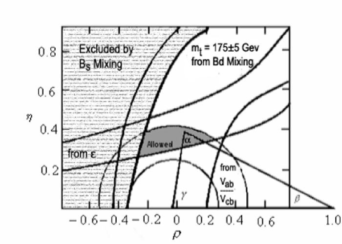
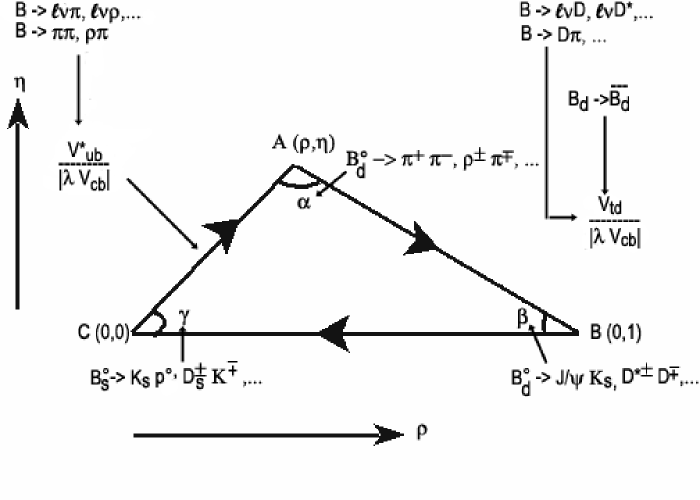
Figure 1: (a) Allowed region for the apex ($\rho,\eta$) of the unitary triangle. (b) Processes to determine the profile of unitary triangle.

Also, the length of the adjacent side connecting ($\rho,\eta$) to (1,0) is essentially determined by the measurement of $B_{d}$ mixing that can provide the value of $V_{td}$. Since the value of $V_{cb}$ is very close to that of $V_{ts}$, one can further constrain this length between ($\rho,\eta$) to (1,0) by measuring the $B_{s}$ mixing. The rainbow around (1,0) shown in Fig. 1(a) corresponds to the allowed region for this length. The overlap of the two rainbows is further constrained by the measurement of CP-violation parameter $\epsilon$ in $K^{0}$-$\bar{K^{0}}$ mixing. Since $\epsilon$ is a direct measure of the complex phase in $V_{CKM}$, the constraint from $K^{0}$-$\bar{K^{0}}$ mixing is drawn as a horizontal band in Fig. 1(a) depending mostly on the value of $\eta$. The final overlap yields then the allowed region for the apex ($\rho,\eta$) of the triangle as shown in Fig. 1(a). The three angles of the triangle denoted by $\alpha,\beta,\gamma$ are given by

$$\alpha={\rm arg}\left(-\frac{V_{td}V_{tb}^{*}}{V_{ud}V_{ub}^{*}}\right),\beta={\rm arg}\left(-\frac{V_{cd}V_{cb}^{*}}{V_{td}V_{tb}^{*}}\right),\gamma={\rm arg}\left(-\frac{V_{ud}V_{ub}^{*}}{V_{cd}V_{cb}^{*}}\right).$$ (13)

It is very interesting to note that these angles can also be determined from the CP-asymmetry measurement [7]. The CP-asymmetry is given by

$$A_{f_{CP}}(t) = \frac{\Gamma(B^{0}_{\rm phys}(t)\to f_{CP})-\Gamma(\bar{B^{0}}_{\rm phys}(t)\to f_{CP})}{\Gamma(B^{0}_{\rm phys}(t)\to f_{CP})+\Gamma(\bar{B^{0}}_{\rm phys}(t)\to f_{CP})},$$

$${\approx} -{\rm Im}\left(\frac{q}{p}\cdot\frac{\bar{\mathcal{M}}}{\mathcal{M}}\right)\sin(\Delta Mt),$$

where $|B_{L}\rangle=p|B^{0}\rangle+q|\bar{B^{0}}\rangle$, $|B_{H}\rangle=p|B^{0}\rangle-q|\bar{B^{0}}\rangle$, ${\mathcal{M}}=\langle f_{CP}|{\mathcal{H}}|B^{0}\rangle$, and $\bar{{\mathcal{M}}}=\langle f_{CP}|{\mathcal{H}}|\bar{B^{0}}\rangle$. From the experimental measurements of $A_{f_{CP}}(t)$, it may be possible to determine the values of angles $\alpha,\beta,\gamma$. For example, the value of $\beta$ may be determined by the measurement of $B_{d}^{0}\to J/\psi K_{s}$. More examples of process to determine each angle are shown in Fig. 1(b). Figure 1(b) also shows other processes to fix the profile of the unitary triangle.

The theoretical efforts in the $B$ physics have also been very extensive in the last twenty years and we cannot summarize all the developments in this talk. Perhaps, here we are just content with a very brief survey. In early 80’s, the value of $V_{cb}$ was investigated significantly with the QCD improved spectator model developed by Altarelli et al. [8]. In the middle of 80’s, a model wavefunction due to Wirbel, Stech and Bauer called WSB model [9] was introduced for the heavy quark system. Then, in the late 80’s, the heavy quark symmetry was extensively studied by many authors [4, 5]. Perhaps, the most quoted work has been done by Isgur and Wise [4] introducing the Isgur-Wise function now frequently referred in the heavy quark effective theory (HQET). The basic idea of heavy quark symmetry is to realize the hidden symmetry of QCD that can be revealed only in the limit of infinitely heavy quark masses. The analogous observation in the opposite extreme of zero quark mass limit is the chiral symmetry. Whether the quark masses are heavy or light may be categorized by the QCD scale $\Lambda_{QCD}$. The current quark masses of $u,d,s$ are much smaller than $\Lambda_{QCD}$, while the masses of $c,b,t$ quarks are much larger than $\Lambda_{QCD}$, i.e. $m_{u},m_{d},m_{s}<<\Lambda_{QCD}<<m_{c},m_{b},m_{t}$. Thus, in the limit that $m_{u},m_{d}$ and $m_{s}$ go to zero, the QCD reveals the chiral symmetry $SU(3)_{L}\times SU(3)_{R}$ and the symmetry is spontaneously broken to $SU(3)_{V}$ due to the non-trivial QCD vacuum. Similarly, in the limit that $m_{c},m_{b}$ and $m_{t}$ go to infinity, the heavy quark symmetry $SU(6)$(or $SU(2N_{f})$) is revealed in QCD.

In the early 90’s, the HQET was applied extensively in the heavy quark systems. At the same time, the constituent quark model(CQM) was built by Isgur, Scora, Grinstein and Wise and named as ISGW model [10]. This model emphasizes the importance of resonance contribution near the small invariant mass of final states in the inclusive semileptonic decays. In the case of semileptonic $B$ decay such as $B\rightarrow e\nu cd$, the invariant mass square $P_{X}^{2}=m_{X}^{2}=(p_{B}-p_{e}-p_{\nu})^{2}$ of the final state, continuum $c$ and $d$ quarks, is bound by $(m_{c}+m_{d})^{2}<P^{2}_{X}<(m_{c}+m_{d})^{2}+(m_{d}/m_{b})(m_{b}-m_{c})$, where $p_{e},p_{\nu}$ and $p_{B}$ are the four-momenta of electron, neutrino and the $B$ meson, respectively. ISGW criticized the early QCD improved spectator model by Altarelli et. al. [8] because the region of $P_{X}^{2}\approx(m_{c}+m_{d})^{2}$ is dominated by the resonances rather than the continuum. In the middle of 90’s, ISGW model was extended to a relativistic version and called ISGW2 model [11]. Throughout 90’s, the lattice QCD [12] was also extensively used to analyze the heavy quark systems. In 90’s, the perturbative QCD(PQCD) [13] approach was used mainly to analyze the hadronic decays of heavy mesons. Then, in the later part of 90’s, dispersion relation was used for the analysis of timelike region using the inputs from CQM [14], lattice data [15], HQET and PQCD [16]. The light-cone quark model(LCQM) was developed around this time. Perhaps, we may categorize the LCQM into four different versions. First, the ISGW2 model was extended to the LC formalism [17]. However, the same input parameters as the ISGW2 model were used in this LCQM. Second, the LC version of HQET was developed [18]. In this development, the WSB model developed in the middle of 80’s was ruled out because the WSB model doesn’t satisfy the constraint from the heavy quark symmetry. Third, the LC model wavefunction was also introduced [19]. However, modelling the LC wavefunction didn’t give any information about the hadron spectra. Finally, we have implemented the variational principle to the QCD motivated effective LC hamiltonian to enable the analysis of meson spectra as well as many wavefunction-related observables such as the form factors, decay constants and electroweak decay rates, etc. [20, 21]. In late 90’s, also other approaches such as the light-cone QCD sum-rule [22], the Dyson-Schwinger equation [23] and the Bethe-Salpeter equation [24] were used to analyze the heavy quark systems. More recently, the quark-meson model [25] utilizing both HQET and chrial perturbation ($\chi_{PT}$) theory was used to analyze the heavy-to-light meson decays such as $B\rightarrow(\pi,\rho,a_{1})\nu l$. In the twenty years of $B$-physics history, we may note that one of the focal point in most analyses has been the accurate prediction of exclusive semileptonic decays such as $B\rightarrow(D,\pi)l\nu$ and $D\rightarrow(K,\pi)l\nu$. In the next section, we now present some more details of exclusive semileptonic decays.

3 Exclusive Semileptonic Decays

The current matrix element of the semileptonic pseudoscalar to pseudoscalar (PS$\to$PS) meson decays involve the two form factors:

$$\langle p_{2}|V^{\mu}|p_{1}\rangle = f_{+}(q^{2})(p_{1}+p_{2})^{\mu}+f_{-}(q^{2})(p_{1}-p_{2})^{\mu}$$

$$= f_{+}(q^{2})\biggl{[}(p_{1}+p_{2})^{\mu}-\frac{M_{1}^{2}-m_{2}^{2}}{q^{2}}q^{\mu}\biggr{]}+f_{0}(q^{2})\frac{M_{1}^{2}-M_{2}^{2}}{q^{2}}q^{\mu}$$

$$= \sqrt{M_{1}M_{2}}[h_{+}(q^{2})(v_{1}+v_{2})^{\mu}+h_{-}(q^{2})(v_{1}-v_{2})^{\mu}],$$

(16)

where

$$f_{0}(q^{2})=f_{+}(q^{2})+\frac{q^{2}}{M_{1}^{2}-M_{2}^{2}}f_{-}(q^{2}).$$ (17)

In the limit of $M_{1,2}\rightarrow\infty$, the only one form factor remains, i.e. $h_{+}(q^{2})=\xi(v_{1}\cdot v_{2})$ and $h_{-}(q^{2})=0$, where $\xi(v_{1}\cdot v_{2})$ is known as the Isgur-Wise function. Also, due to the Ademello-Gatto theorem [26], $f_{+}(0)\approx 1$. Note here that $f_{+}(q^{2})$ corresponds to the charge form factor in the $SU(3)$ limit. The similar decomposition of the matrix element of the semileptonic pseudoscalar (PS) to vector (V) meson decays can be made with the four transition form factors. Again in the heavy quark mass limit, only one form factor $\xi(v_{1}\cdot v_{2})$ is needed. Also, the Luke theorem [27] applies in the zero recoil limit. However, because of the limited space, we won’t discuss the details of PS$\to$V semileptonic decays in this presentation but here focus only on the PS$\to$PS semleptonic decays.

The analysis of exclusive processes can be made efficiently in the LC formalism with the rational energy-momentum relation. In the LCQM calculations presented in Ref. [17], the $q^{+}\neq 0$ frame has been used to calculate the weak decays in the timelike region $m^{2}_{\ell}\leq q^{2}\leq(M_{1}-M_{2})^{2}$, with $M_{1(2)}$ and $m_{\ell}$ being the initial (final) meson mass and the lepton ($\ell$) mass, respectively. However, when the $q^{+}\neq 0$ frame is used, the inclusion of the nonvalence contributions arising from quark-antiquark pair creation (“Z-graph”) is inevitable and this inclusion may be very important for the heavy-to-light and light-to-light decays. Nevertheless, the previous analyses [17] in the $q^{+}\neq 0$ frame considered only valence contributions neglecting the nonvalence contributions.

Figure 2: Effective calculation of the embedded state (black blob) in terms of the usual LC wave fucntion (white blob).

In this work, we treat the nonvalence state using the Schwinger-Dyson equation to connect the embedded-state shown as the black blob in Fig. 2 to the ordinary LC wave function (white blob in Fig. 2). To make the program successful, we need some relevant operator connecting one-body to three-body sector shown as the black box in Fig. 2. The relevant operator is in general dependent on the involved momenta. Our main observation is that we can remove the four-body energy denomenator $D_{4}$ using the identity $1/D_{4}D^{\gamma}_{2}+1/D_{4}D^{h}_{2}=1/D^{\gamma}_{2}D^{h}_{2}$ of the energy denominators and obtain the identical amplitude in terms of ordinary LC wave functions of photon and hadron (white blob). For the small momentum transfer, perhaps the relevant operator may not have too much dependence on the involved momenta and one may approximate it as a constant operator. In contact interaction case, we verified that our prescription of a constant operator in Fig. 2(d) is an exact solution of Fig. 2(a). In our previous analysis [21] for the exclusive PS$\to$PS semileptonic decays, the form factor $f_{+}(q^{2})$ obtained from $j^{+}$ in $q^{+}=0$ frame is not only immune to the zero-mode contribution but also in good agreement with the experimental data as well as other theoretical results. In order to obtain the form factor $f_{-}$ in $q^{+}=0$ frame, one has to use another component (i.e. $j_{\perp}$ or $j_{-}$) of the current in addition to the $j^{+}$. However, as noted in Ref. [28], those $j_{\perp}$ and $j_{-}$ are not immune to the zero-mode contributions, which are not easy to be identified in LCQM. Thus, we use $q^{+}\neq 0$ frame to determine the constant operator by equating the slope of $f_{+}$ at $q^{2}=0$ in $q^{+}\neq 0$ frame to that in $q^{+}=0$ frame. Then, we apply the same operator to the calculation of $f_{-}$. We present here some preliminery results for $K_{\ell 3}$ using the approximation of constant operator to illustrate our method.

Table 1: Preliminary results for the parameters of $K^{0}_{\ell 3}$ decay form factors.

	$q^{+}\neq 0$ frame		$q^{+}=0$ frame
	Effective(val + nv)	valence	valence	Experiment [2]
$f_{+}(0)$	0.962	0.962	0.962
$\lambda_{+}$	0.026	0.083	0.026	$0.0288\pm 0.0015[K^{0}_{e3}]$
$\lambda_{0}$	0.025	$-0.017$	0.001	$0.025\pm 0.006[K^{0}_{\mu 3}]$
$\xi_{A}$	$-0.013$	$-1.10$	$-0.29$	$-0.11\pm 0.09[K^{0}_{\mu 3}]$

In Table 1, we summarize the experimental observables for the $K_{\ell 3}$ decays, where $\lambda_{i}=M^{2}_{\pi}f^{\prime}_{i}(0)/f_{i}(0)(i=+,0)$ and $\xi_{A}=f_{-}(0)/f_{+}(0)$. We use our linear potential parameters given by Refs. [20, 21] in this analysis. As one can see in Table 1, our results for the slope $\lambda_{0}$ of $f_{0}$ at $q^{2}=0$ and $\xi_{A}$=$f_{-}(0)/f_{+}(0)$ are now much improved and comparable with the data. Especially, our result of $\lambda_{0}$= 0.025 obtained from our effective calculation is in excellent agreement with the data, $\lambda^{\rm Exp.}_{0}$=0.025$\pm$0.006. More theoretical details on our effective method as well as heavy-to-heavy and heavy-to-light semileptonic processes will be presented in the future communication.

4 Conclusion

With the wealth of new or upgraded experimental facilities, precision test of standard model is ever more promising. We presented a theoretical overview of B-physics and noted that the exclusive semileptonic B-decays and rare B-decays are very important to determine $V_{bc}$, $V_{bu}$, $V_{td}$, $V_{ts}$, and $V_{tb}$ stringently. As we discussed, an effective use of LC degrees of freedom seems crucial to make predictions consistent with many other exclusive processes. Our initial attempt to accomodate the contributions from embedded states seems to give encouraging results.

We would like to thank Prof. Chris Pauli for organizing a stimulating meeting and his outstanding hospitality at the Max Plank Institute. We also thank Chirag Lakhani for drawing a figure. This work was supported by a grant from the U.S. DOE under contracts DE-FG02-96ER40947.

References

- [1] For the experimental overview of B-physics, see H. Schröder in this proceedings.
- [2] Particle Data Group, D. E. Groom et al., Eur. Phys. J. C 15 (2000) 1.
- [3] L. Wolfenstein, Phys. Rev. Lett. 51 (1983) 1945.
- [4] N. Isgur and M. B. Wise, Phys. Lett. B 232 (1989) 113; Phys. Lett. B 237 (1990) 527.
- [5] E. E. Eichten and B. Hill, Phys. Lett. B 234 (1990) 511; M. Neubert, Phys. Lett. B 338 (1994) 841.
- [6] CLEO Collab. R. Ammar et al., Phys. Rev. Lett. 71 (1993) 674.
- [7] See e.g. Y. Nir and H. R. Quinn, in B Decays (revised 2nd Edition) edited by S. Stone, World Scientific, Singapore, 1994.
- [8] G. Altarelli, M. Cabibbo, G. Corbo, and L. Maiani, Nucl. Phys. B 207 (1982) 35; N. Cabibbo, G. Corbo, and L. Maiani, . B 155 (1979) 93.
- [9] M. Wirbel, B. Stech and M. Bauer, Z. Phys. C 29 (1985) 637.
- [10] N. Isgur, D. Scora, B. Ginstein, M. B. Wise, Phys. Rev. D 39 (1989) 799.
- [11] D. Scora and N. Isgur, Phys. Rev. D 52 (1995) 2783.
- [12] J. M. Flynn and C. T. Sachrajda, Heavy Quark Physics From Lattice QCD, to appear in Heavy Flavor, 2nd ed., A. J. Buras, M. Lindner (Eds.), World Scientific, Singapore, hep-lat/9710057; C. W. Bernard, A. X. El-Khadra, and A. Soni, Phys. Rev. D 43 (1991) 2140; . D 45 (1992) 869; UKQCD Collaboration, K. C. Bowler et al., Phys. Rev. D 51 (1995) 4905.
- [13] A. Szczepaniak, E. M. Henley, and S. J. Brodsky, Phys. Lett. B 243 (1990) 287; C. E. Carlson and J. Milana, Phys. Rev. D 49 (1994) 5908.
- [14] D. Melikhov, Phys. Rev. D 53 (1996) 2460.
- [15] D. Becirevic, Phys. Rev. D 54 (1996) 6842.
- [16] C. G. Boyd, B. Grinstein and R. F. Lebed, Phys. Rev. D 56 (1997) 6895.
- [17] I. L. Grach, I. M. Narodetskii, and S. Simula, Phys. Lett. B 385 (1996) 317; F. Cardarelli and S. Simula, Phys. Lett. B 421 (1998) 295.
- [18] H.-Y. Cheng, C.-Y. Cheung, C.-W. Hwang, and W.-M. Zhang, Phys. Rev. D 57 (1998) 5598. Phys. Rev. D 52 (1995) 2915.
- [19] W. Jaus, Phys. Rev. D 53 (1996) 1349.
- [20] H. -M. Choi and C. -R. Ji, Phys. Rev. D 59 (1999) 074015.
- [21] H. -M. Choi and C. -R. Ji, Phys. Rev. D 59 (1999) 034001; Phys. Lett. B 460 (1999) 461.
- [22] P. Ball and V. M. Braun, Phys. Rev. D 58 (1998) 094016; T. M. Aliev and M. Savic, J. Phys. G 24 (1998) 2223.
- [23] M. A. Ivanaov, Yu. L. Kalinovsky and C. D. Roberts, Phys. Rev. D 60 (1999) 034018.
- [24] H.-W. Huang, Phys. Rev. D 56 (1997) 1579.
- [25] A. Deandrea, R. Gatto, G. Nardulli, and A. D. Polosa, Phys. Rev. D 59 (1999) 074012.
- [26] M. Ademollo and R. Gatto, Phys. Rev. Lett. 13 (1964) 264.
- [27] M. E. Luke, Phys. Lett. B 252 (1990) 447.
- [28] W. Jaus, Phys. Rev. D 60 (1999) 054026.