The $g$ Factor of a Bound Electron
in a Hydrogen-Like Atom

Abstract

Recently, a precise measurement on the bound electron $g$ factor in hydrogen-like carbon was performed werth . We consider the present status of the theory of the $g$ factor of an electron bound in a hydrogen-like atom and discuss new opportunities and possible applications of the recent experiment.

1 Introduction

Until now any precision test of bound state QED icap was always realized in the way that only a final theoretical figure could be compared with some experimental result and no term of any theoretical expression could be tested separately. Any theoretical expression is a function of few parameters and one of them is the nuclear charge $Z$. However, there was no way to measure any function of $Z$. Only very few particular values of $Z$ were available for precision experiments of the Lamb shift, fine and hyperfine structure. Now this has been changed dramatically.

Recently a bound electron $g$ factor in the hydrogen-like carbon ion was measured very accurately by the Mainz-GSI collaboration werth . We consider here this new opportunity to test bound state QED and to determine precisely some fundamental constants from the study of the bound electron $g$ factor.

In contrast to the study of the Lamb shift and hyperfine structure, it is possible to perform experiments on the $g$ factor of the bound electron in different hydrogen-like ions with about the same accuracy. The experiment [1] is now in progress and some other hydrogen-like ions can be measured soon. This provides a possibility to learn about the bound $g$ factor as a function of the nuclear charge $Z$ and the nuclear mass number $A$. The ions under study werth must have spinless nuclei and so they have the most simple level scheme.

The measured value is equal to $(Z-1)m/gM$, where $m$ is the electron mass, and $M$ is the nuclear mass. The latter is usually known accurately in atomic mass units. If we determine the bound electron $g$ factor from the theory, then the experiment leads to a new precision value of the electron mass in atomic units. The accuracy of the electron mass value is compatible with the one from a direct measurement mass . The uncertainty of the theory of the $g$ factor in the carbon ion is on about the same level as the experimental one. The theoretical precision can be improved if the berillium ion, where the only unknown correction $(Z\alpha)^{4}m/M$ is small and negligible, is studied.

Another way to manage experimentally the problem of the unknown term is to use another kind of theory. The usual theory in the case of simple atoms (we call it strong theory) give us some values, while in case of the $g$ factor it must be useful even to fix a form of the theoretical expression (we call this option weak theory). When one knows part of the theoretical terms and a form of other terms, it is possible try to measure the unknown coefficients. The only unknown term which is important for carbon and ions with $Z$ around 6 is of order $(Z\alpha)^{4}m/M$. One can take an advantage of the weak theory approach and measure the coefficient of this term by studying with the oxygen ion.

An important feature of the study of the $g$ factor of a bound electron at $Z=20-30$ is also the possibility to learn about higher-order two-loop corrections, which are one of the crucial problems of bound state QED theory. Below we discuss in detail the present status of theory and experiment. We consider a new opportunity to precisely test bound state QED and to accurately determine two fundamental constants: the electron-to-proton mass ratio and the fine structure constant.

Below we discuss in detail a number of problems arising due to the precision study of the bound electron $g$ factor.

2 Theory

2.1 Present status

We follow the notation of our paper PLA and present the $g$ factor of a bound electron in a hydrogen-like ion in the form

$$g_{e}=2\cdot(1+a+b)$$ (1)

where the bound electron anomalous magnetic moment at low $Z$ is $b\sim(Z\alpha)^{2}$, while the free part of the anomalous magnetic moment is $a\sim\alpha/2\pi$. It is useful to split the bound-state electron anomaly into three terms PLA :

$$b=1\cdot b_{1}+a\cdot b_{a}+b^{\prime}\;,$$ (2)

where two first terms kin1 ; kin2

$$b_{1} = \frac{1+2\sqrt{1-(Z\alpha)^{2}}}{2}+(Z\alpha)^{2}\left[\frac{1}{2}\frac{m}{M}-\frac{1+Z}{2}\left(\frac{m}{M}\right)^{2}\right]$$ (3)

$$\simeq (Z\alpha)^{2}\left[-\frac{1}{3}+\frac{1}{2}\frac{m}{M}-\frac{1+Z}{2}\left(\frac{m}{M}\right)^{2}-\frac{1}{12}(Z\alpha)^{2}\right]$$ (4)

and kin1a ; kin2

$$b_{a}=(Z\alpha)^{2}\left[\frac{1}{6}-\frac{1}{3}\frac{m}{M}\right]$$ (5)

are due to kinematic effects, while the last term is due to some non-trivial bound-states effects. The $b^{\prime}$ term starts from the order of $(Z\alpha)^{4}$ and contains QED ($\alpha(Z\alpha)^{4}m$ and higher) BCS ; PSSL ; beier , nuclear size ($(Z\alpha)^{4}(mR_{N})^{2}$ and higher) PSSL and recoil ($(Z\alpha)^{4}m/M$ and higher) corrections. In Table 1 we present the most accurate published values PSSL of different contributions to $b^{\prime}$. The uncertainty was not specified there and we estimate it as half the value of the last digit. More precise calculations are presented in Ref. beier .

Table 1: Some contributions to $b^{\prime}$ in units of $10^{-9}$ PSSL due to vacuum polarization ($VP$), self-energy ($SE$) and finite nuclear size ($NS$). The nuclear size effects were studied there for the main isotope of each element

$Z$	$b^{\prime}_{\rm VP}~{}~{}~{}~{}$	$b^{\prime}_{\rm SE}~{}~{}~{}~{}~{}$	$b^{\prime}_{\rm NS}~{}~{}~{}$
1	-0.00(3)	0.08(3)
2	-0.05(3)	0.93(3)
4	-0.86(3)	12.77(3)
6	-4.2(3)	55.2(3)
8	-13.2(3)	151.4(3)	0(7)
10	-31.8(3)	327.1(3)	0(7)
12	-64.6(3)	610.9(3)	5(7)
14	-118(3)	1 030(3)	10(7)
16	-200(3)	1 610(3)	20(7)
18	-309(3)	2 381(3)	35(7)
24	-948(3)	6 127(3)	135(7)
32	-2 890(3)	16 808(30)	620(70)

2.2 Comparison to the experiment

Precision studies of the $g$ factor of a bound electron in simple atoms were started with experiments on hydrogen h and its comparison with deuterium d1 ; d2 ; d3 and tritium t , as well as on the helium ion he . In particular in case of low $Z$ the result for the non-trivial bound-state term

$$b^{\prime}(Z=1)=0.1\cdot 10^{-9}$$ (6)

and

$$b^{\prime}(Z=2)=0.9\cdot 10^{-9}$$ (7)

is small enough and that explains why experimental results from the precision measurements done decadse ago have been out of the theoretical interest for two last decades.

We summarize experimental and theoretical data in Table 2. Some of them were obtained indirectly and we present in Appendix Table 5 all important auxiliary measurements.

Table 2: Comparison of theory and experiment. Here, $g_{0}(e)$ stands for the magnetic moment of a free electron and it contains the anomalous magnetic moment $a\sim\alpha/2\pi$

Value	Experiment	Reference	Theory
$\frac{g({\rm H})}{g_{0}(e)}$	$1-17.709(13)\cdot 10^{-6}$	h ; d1	$1-17.694\cdot 10^{-6}$
$\frac{g({\rm D})}{g({\rm H})}$	$1-7.22(3)\cdot 10^{-6}$	d3	$1-7.24\cdot 10^{-6}$
$\frac{g({\rm T})}{g({\rm H})}$	$1-10.7(15)\cdot 10^{-6}$	t	$1-9.7\cdot 10^{-6}$
$\frac{g({}^{4}{\rm He}^{+})}{g_{0}(e)}$	$1-70.88(30)\cdot 10^{-6}$	d1 ; h ; he ; rb87 ; rb85 ; 8785	$1-70.91\cdot 10^{-6}$
$\frac{g({}^{12}_{~{}6}{\rm C}^{5+})}{2}$	$1+520.798(2)\cdot 10^{-6}$	werth	$1+520.795(1)\cdot 10^{-6}$

In the case of the recent experiment with hydrogen-like carbon the non-trivial QED effects contribute an observable amount (see Table 1). We need to mention that, due to some delay of the final publications of the experimental result werth and theoretical calculations beier , no actual theoretical predictions have been published. Most of the presentations (conference and seminar talks and posters) dealt with unaccurate theoretical predictions because it was believed that nothing had been known on the two-loop corrections. However, that was not the case, because from the beginning of the theoretical calculations up to recent re-calculations it was clearly stated ed kin1a that the $(Z\alpha)^{2}$ term in Eq. (5) is of pure kinematic origin and so the result is valid in any order of the expansion in $\alpha$ for the anomalous magnetic moment of a free electron, and in particular

$$\Delta b({\rm two-loop}) \simeq \left[-0.328...\left(\frac{\alpha}{\pi}\right)^{2}\right]\left[\frac{1}{6}(Z\alpha)^{2}\right]$$ (8)

$$= -5.7\cdot 10^{-10}\;.$$ (9)

We also confirmed this statement in our paper PLA . Our use of the known result on the $\alpha^{2}(Z\alpha)^{2}$ term leads to

$$b({}^{12}_{~{}6}{\rm C}^{5+})=1+520\,795(1)\cdot 10^{-9}$$ (10)

and offers the accuracy presented in Table 2.

2.3 Potential model

The bound $g$ factor is now a new value that must to be precisely calculated and it may be useful to compare the calculation of the $g$ factor with evalutions for the energy levels. A number of corrections can be described with the help of an effective potential, and in particular effects due to vacuum polarization of free electrons, the Wichmann-Kroll potential and nuclear size can be studied in the leading non-relativistic approximation with the use of a delta-like potential

$$V({\bf r})=A\delta({\bf r})\;,$$ (11)

where the energy shift of the ground state due to this potential is of the form

$$\Delta E_{A}=A\,\frac{(Z\alpha m)^{3}}{\pi}$$ (12)

and for different corrections the shift is

$$\Delta E_{VP} = -\frac{4}{15}\frac{\alpha(Z\alpha)^{4}m}{\pi}\;,$$ (13)

$$\Delta E_{WK} = \left(\frac{19}{45}-\frac{\pi^{2}}{27}\right)\frac{\alpha(Z\alpha)^{6}m}{\pi}\;,$$ (14)

$$\Delta E_{NS} = \frac{2}{3}\,\frac{(Z\alpha)^{4}m}{\pi}\,(mR_{N})^{2}\;.$$ (15)

We have calculated a correction to the bound electron anomaly and the result is PLA

$$\Delta b^{\prime}_{A}=2\,\frac{\Delta E_{A}}{m}\;.$$ (16)

In particular, for the finite-nuclear-size correction one obtains

$$\Delta b^{\prime}_{NS} = \frac{4}{3}\,(Z\alpha)^{4}\,(mR_{N})^{2}$$ (17)

$$\simeq 2.5355\cdot 10^{-14}\,Z^{4}\,{\cal R}^{2}\;,$$ (18)

where the value root-mean-square charge radius ${\cal R}$ in fermi for carbon ¹²C is equal to 2.478(6) RC12 and

$$\Delta b^{\prime}_{NS}(^{12}{\rm C}^{5+})=0.2\cdot 10^{-9}\;.$$ (19)

Our results are in agreement with direct numerical calculations for several corrections PSSL (see Tables 3 and 4). Eq. (16) can be used to estimate unknown corrections if we know the energy shift. Actually we put in Tables 3 and 4 the uncertainty of the analytic results found in this way PLA . However, one has to remember that the theory of the bound $g$ factor is more complicated than the one for the Lamb shift and sometimes the bound anomaly can be more logarithmic. An example is the order $\alpha^{2}(Z\alpha)^{4}$: the $b^{\prime}$ term contains a logarithm of $(Z\alpha)$ and a non-analytic contribution due to low energy effects, while the contribution to the Lamb shift in this order has no logarithm and completely originates from the high energy contribution. Higher-order two-loop terms have not been evaluated yet even in the case of the energy levels of low-$Z$ atoms, and we do not anticipate the results in near future. As we mentioned, the bound $g$ factor involve more complicated calculations than the theory of energy levels, and a reason of our study using effective non-relativistic technics is to find an appropriate approach for effective $(Z\alpha)$ expansions which can be used to study two-loop corrections.

Table 3: Comparison of the vacuum polarization contribution: Eq. (16) against PSSL . The uncertainty of the analytic result was discussed in Ref. PLA

$Z$	Numerical result	Analytic result
	Ref. PSSL	Eq. (16)
	$[10^{-9}]$	$[10^{-9}]$
1	-0.00(1)	-0.003 5
2	-0.05(1)	-0.056(1)
4	-0.86(1)	-0.90(3)
6	-4.2(1)	-4.6(2)
8	-13.2(1)	-14(1)
10	-31.8(1)	-35(3)
12	-64.6(1)	-73(8)
14	-118(1)	-135(17)
16	-200(1)	-230(33)
18	-309(1)	-369(59)
20		-560(100)
22		-830(160)
24	-948(1)	-1 170(250)
26		-1 600(370)
28		-2 160(540)
30		-2 850(760)
32	-2 890(1)	-3 680(1 060)

Table 4: Finite-nuclear-size contribution: Eq. (16) against PSSL . The uncertainty of the analytic result was discussed in Ref. PLA

$Z$	$R_{N}$	Numerical result	Analytic result
		Ref. PSSL	Eq. (16)
	[fm]	$[10^{-9}]$	$[10^{-9}]$
8	2.737(8)	0(3)	0.78(6)
10	2.992(8)	0(3)	2.27(9)
12	3.08(5)	5(3)	5.0(3)
14	3.086(18)	10(3)	9.2(7)
16	3.230(5)	20(3)	17(2)
18	3.423(14)	35(3)	31(4)
24	3.643(3)	135(3)	112(22)
32	4.088(8)	620(3)	444(145)

3 Precise tests of the bound state QED

Now let us discuss possible precision tests of bound state QED. First we need to discuss what experimental results have been available up-to-now icap :

• Precision measurements of the Lamb shift are possible for $Z=1,2$.

• The fine structure can be precisely studied for $Z=1$ and $Z=6$.

• Transitions in the gross structure can be accurately measured at $Z=1,2$.

• The hyperfine structure of the 1s and 2s levels can be obtained precisely for the hydrogen atom and its isotops and for the helium-3 ion.

• Precise measurements are also possible for a few transitions in helium.

• In the case of some high-$Z$ ions, precision experiments are also possible.

Now we list the accurate theoretical predictions that have been available icap up-to-date:

• Accurate calculations for the Lamb shift and hfs of hydrogen-like atoms are limited by their nuclear structure and higher-order QED corrections. In the case of low-$Z$ Lamb shift, the finite-nuclear-size effects can be taken into account easily if we know the nuclear charge radius.

• In the case of some high-$Z$ experiments the uncertainty due to the nuclear structure disturbs any interpretations in terms of a test of quantum electrodynamics. However, the QED calculations are still important for the study of nuclear structure.

• Few-electron atomic systems cannot be precisely calculated at low $Z$, except some special cases (like e. g. isotopic shift).

• In the case of high-$Z$ few-electron ions, one of theoretical problems is the higher-order electron-electron interaction.

Summarizing this section we need to underline that only a few of values of $Z$ are available for the precision experiment, a comparison of experiment and theory can be done only for the final values and there is a problem of theoretical uncertainty due to unknown higher-order corrections, which cannot be calculated at the moment. We call a theory, which predicts only an final value to be compared with an experiment, a strong theory.

3.1 Weak and strong theory

The study of the bound electron $g$ factor provides another option. It is possible now to check a part of the theoretical expression. The expression is a function of the nuclear charge ($Z$), the atomic mass ($A$) and the nuclear charge radius ($R_{N}$). The nuclear effects can be easily calculated in the leading order if the nuclear radius is known. Since it is possible to measure the $g$ factor for different values of $Z$ and $A$, the complete functions can be now available. We put in Fig. 1 all spinless nuclei with a not too high value of $Z$ for hydrogen-like ($Z^{*}=Z$) and lithium-like ions ($Z^{*}=Z-2$). The use of ions with different values of the charge-to-mass ratio can be also helpful to learn about systematic errors. Due to that it seems to be important to understand which progress in calculations for light and medium lithium-like ions is possible in near future.

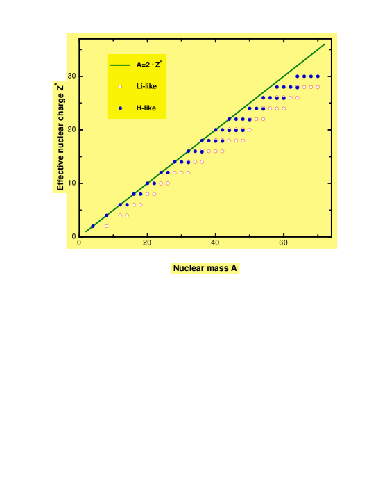
Figure 1: Hydrogen-like and lithium-like ions with spinless nuclei

Such a situation with a broad range of available values of $Z$ and $A$ offers a different way to compare theory and experiment. It is possible now to compare a theoretical expression, which is known only partially, but with a form of unknown coefficients which is completely understood. For example one can write for $Z\sim 6$

$$g_{e}(Z)=g_{\rm known}(Z)+C\,(Z\alpha)^{4}\frac{m}{M}\;,$$ (20)

where the first term is known. Studying experimentally carbon and oxygen the unknown coefficient $C$ can be determined. We call this way to use theory a weak theory.

3.2 Higher-order two-loop contributions

When we go to a higher value of $Z$ ($Z\sim 20$) a wide set of unknown terms have to be taken into account. First we need to study all coefficients in equation

$$C_{0}\,(Z\alpha)^{4}\frac{m}{M} + C_{1}\,\alpha(Z\alpha)^{4}\ln(Z\alpha)+C_{2}\,\alpha(Z\alpha)^{4}$$ (21)

$$+ C_{3}\,(Z\alpha)^{5}\frac{m}{M}\ln(Z\alpha)+C_{4}\,(Z\alpha)^{5}\frac{m}{M}+C_{5}\,\alpha^{2}(Z\alpha)^{5}\;.$$ (22)

These coefficients can be studied at $Z=10-20$ or calculated. With $Z$ higher than 20 it is necessary to take into consideration $\alpha^{2}(Z\alpha)^{6}$ terms which can contain temrs up to the cube of the low-energy logarithm ($\ln(Z\alpha)$) and we have a problem of higher-order two-loop corrections. That is now one of the most important theoretical problems in bound-state QED. In particular, it essentially limits computational accuracy for

• the hydrogen Lamb shift, fine and gross structure;

• the hyperfine structure intervals in hydrogen, deuterium and especially in the ³He⁺ ion (namely, some special combination of that for 1s and 2s levels ks );

• the Lamb shift and gross structure in the helium-4 ion;

• the fine structure in hydrogen-like nitrogen;

• high-$Z$ few electron atoms (rather “exact” calculation in $(Z\alpha)$ is needed).

In the case of the bound $g$ factor for the first time there is an opportunity to study the higher-order two-loop corrections experimentally in detail with varying value of $Z$.

3.3 Physics of medium $Z$

The possibility of the direct experimental study of these higher-order two-loop terms shows the importance of physics of moderate $Z$. Medium-$Z$ theory provides a possibility to develop both high-$Z$ and low-$Z$ approaches. In case of low-$Z$ technics, one can expand over $(Z\alpha)$ and see if our assumptions on higher-order terms is appropriate or not. Using high-$Z$ methods one can perform a $1/Z$ expansion and treat the electron-electron interaction in few-electron ions as a perturbation. The study of the $g$ factor of lithium-like ions offers an experimental test of present ideas on how large higher-order corrections electron-electron interaction can be.

4 Carbon and calcium experiments

4.1 Carbon experiment and electron-to-proton mass ratio

Comparison of theory to precision experiment often involves some other experimental data from different fields. In particular, the $g$ factor experiment werth deals with a comparison of two frequencies: the Larmor spin precession frequency

$$\omega_{\rm L}=g_{e}\,\frac{e}{2\,m\,c}\,B$$ (23)

and the ion cyclotron one

$$\omega_{\rm c}=\frac{(Z-1)\,e}{2\,M_{I}\,c}\,B\;.$$ (24)

They are proportional to the magnetic field $B$, but their ratio is field-independent. Eventually, the experiment leads to a value of $g_{e}M_{I}/m$, where $M_{I}$ is the ion mass. There are three sources of uncertainty involved:

• an experemental for the frequencies $\omega_{\rm L}$ and $\omega_{\rm c}$;

• a computational one for the $g$ factor;

• the one due to the determination of the electron mass $m$ in proper units (either in atomic mass units or in terms of the proton mass).

All of them are comparable werth . The use of theoretical values and the experimental data werth for the frequencies leads to a value of the electron mass.

One source of theoretical uncertainty is the unknown term in order $(Z\alpha)^{4}m/M$ (see Eq. (20)) and it might be helpful to study ⁴He⁺ and ¹⁰Be (the correction is negligible) or ¹⁶O and ¹⁸O (the correction is 2.4 and 2.1 times larger than that for ¹²C). It is important to mention that comparing the results on the $g$ factor at different $Z$ values, one can check the consistency of the theory without using any data of the electron mass. Varying $Z$ ($Z=2,4,6,,8$) one can first fix the only unknown coefficient and then determine the electron mass.

A study of the electron mass is now of interest also because of determination of the fine structure constant $\alpha$ from the photon-recoil-spectroscopy chu ; pritchard . A measurement of the recoil frequency shift

$${\delta\nu\over\nu}=\frac{h\nu}{2M_{A}c^{2}}$$ (25)

where $\nu$ is a transition frequency and $M_{A}$ is an atomic mass, together with a known value of frequency $\nu$ gives a value of $h/M_{A}$. The latter can be compared with the Rydberg constant

$$Ry=\alpha^{2}\,\frac{mc}{h}$$ (26)

and that allows to determine the fine structure constant $\alpha$. The Rydberg constant is known very accurately Ry , the recoil shift ${\Delta\nu/\nu}$ was measured for $D_{1}$ cesium line in Ref. chu , while the frequency of the $D_{1}$ line was determined in Ref. udem . To extract $\alpha$ we also need to know $m/M_{Cs}$. The cesium mass in atomic mass units was obtained in Ref. pritchard . The accuracy of the frequency recoil shift chu is larger, but compatible with the one for the electron mass in atomic units mass . It seems chu that in near future a determination of the fine struture constant from the recoil spectroscopy will be limited by the knowledge of the electron mass.

4.2 Calcium measurement: why it is getting interesting

Another way to obtain the fine structure constant $\alpha$ via the bound electron $g$ factor is to work at higher $Z$. As we mention, the investigation at $Z\sim 20$ and higher can be useful to learn about higher-order two-loop corrections. However, the study offers also a new way to determine the fine structure constant. For the calcium ion ($Z=20$) the bound anomaly $b$ is larger than the free term $a$ and hopefully it is still possible to use an expansion in $(Z\alpha)$. A value of $\alpha$ is to be extracted from $(Z\alpha)^{2}$ term. If a routine work from experimental and theoretical sides (i. e. a measurement in the hydrogen-like calcium ion with an uncertainty on a level of $10^{-9}$ and a computation of QED corrections to the $g$ factor, which are similar to the ones evaluated some time ago for the energy levels) a value of $\alpha$ with uncertainty about $10^{-7}$ can be reached. We expect that an experimental progress is possible and further improvement can be expected.

5 Summary

Concluding our consideration we would like to underline, that the study of the $g$ factor of a bound electron werth offers a new opportunity for us to precisely test bound state QED theory and to determine two important fundamental constants: the fine structure constant $\alpha$ and the electron-to-proton mass ratio $m/m_{p}$. The experiment can be performed at any $Z$ with about the same accuracy werth and one can expect new data at medium $Z$ which will allow to verify the present ability to estimate unknown higher-order corrections (i. e. theoretical uncertainty) in both: low-$Z$ and high-$Z$ calculations.

Aknowledgements

I am grateful to T. Beier, H. Häffner, N. Hermanspahn, V. G. Ivanov, W. Quint, H.-J. Kluge, V. M. Shabaev, J. Reichert, and especially to Günter Werth for stimulating discussions. The work was supported in part by RFBR grant 00-02-16718, NATO grant CRG 960003 and the Russian State Program “Fundamental Metrology”.

Appendix: Auxiliary data on the bound electron $g$ factor measurements

Table 5: Experimental data for the $g$ factor of the hydrogen isotopes and the helium ion

Value	Result	Reference
$\frac{g({}^{87}{\rm Rb},\,5S_{1/2})}{g({\rm H,\,1s})}$	$1+23.585\,5(6)\cdot 10^{-6}$	d1
$\frac{g({}^{87}{\rm Rb},\,5S_{1/2})}{g({\rm D,\,1s})}$	$1+23.592\,7(10)\cdot 10^{-6}$	d1
$\frac{g({}^{87}{\rm Rb},\,5S_{1/2})}{g_{0}}$	$1+5.876(13)\cdot 10^{-6}$	h
$\frac{g({}^{4}{\rm He}^{+},\,1s)}{g({}^{4}{\rm He},\,2^{3}S_{1})}$	$1-29.95(30)\cdot 10^{-6}$	he
$\frac{g({}^{4}{\rm He},\,2^{3}S_{1})}{g({}^{87}{\rm Rb},\,5S_{1/2})}$	$1-46.798(50)\cdot 10^{-6}$	rb87
$\frac{g({}^{4}{\rm He},\,2^{3}S_{1})}{g({}^{85}{\rm Rb},\,5S_{1/2})}$	$1-46.77(7)\cdot 10^{-6}$	rb85
$\frac{g({}^{85}{\rm Rb},\,5S_{1/2})}{g({}^{87}{\rm Rb},\,5S_{1/2})}$	$1-0.000\,41(60)\cdot 10^{-6}$	8785

References

- (1) G. Werth et al., this conference; H. Häffner et al., invited talk at ICAP 2000, to be published
- (2) S. G. Karshenboim, invited talk at ICAP 2000, to be published; e-print hep-ph/0007278
-
(3)
D. L. Farnham, R. S. Van Dyck, Jr., and P. B. Schwinberg,
Phys. Rev. Lett. 75, 3598 (1995);
R. S. Van Dyck, Jr., D. L. Farnham, and P. B. Schwinberg, Phys. Scripta T59, 134 (1995) - (4) S. G. Karshenboim, Phys. Lett. A 266, 380 (2000)
- (5) G. Breit, Nature 122, 649 (1928)
- (6) H. Grotch, Phys. Rev. Lett. 24, 39 (1970)
-
(7)
R. N. Faustov, Nuovo
Cim. 69A (1970) 37; Phys. Lett. 33B, 422 (1970);
H. Grotch, Phys. Rev. A2, 1605 (1970);
H. Grotch and R. A. Hegstrom, Phys. Rev. A4, 59 (1971);
see also M. I. Eides and H. Grotch, Ann. Phys. 260, 191 (1997) - (8) S. A. Blundell, K. T. Cheng, and J. Sapirstein, Phys. Rev. A55, 1875 (1997)
- (9) H. Persson, S. Salomonson, P. Sunergren, and I. Lindgren, Phys. Rev. A56, R2499 (1977)
- (10) T. Beier et al., this conference
- (11) J. S. Tideman and H. G. Robinson, in Atomic Physics 7, Plenum Press, 1973, Ed. by S. J. Smith, G. K. Walters and L. H. Volsky, p. 85; Phys. Rev. Lett. 39, 602 (1977)
- (12) W. M. Hughes and H. G. Robinson, Phys. Rev. Lett. 23, 1209 (1969); H. G. Robinson and W. M. Hughes, in Precision Measurement and Fundamental Constants, Washington, NBS spec. publ. 343, Ed. by. D. N. Langenberg and B. N. Taylor, p. 427
- (13) D. J. Larson, P. A. Valberg and N. F. Ramsey, Phys. Rev. Lett. 23, 1369 (1969)
- (14) F. G. Walther, W. D. Phillips and D. Kleppner, Phys. Rev. Lett. 28, 1159 (1972)
- (15) D. J. Larson and N. F. Ramsey, Phys. Rev. A9, 1543 (1974)
- (16) C. E. Johnson and H. G. Robinson, Phys. Rev. Lett. 45, 250 (1980)
- (17) G. M. Keiser, H. G. Robinson and C. E. Johnson, Phys. Rev. Lett. 35, 1223 (1975); Phys. Rev. A16, 822 (1977)
- (18) B. E. Zundell and V. W. Hughes, Phys. Lett. A59, 381 (1976)
- (19) C. W. White, W. M. Hughes, G. S. Hayne, and H. G. Robinson, Phys. Rev. 174, 23 (1968)
- (20) E. A. J. M. Offermann, L. S. Cardman, C. W. de Jager, H. Miska, C. de Vries and H. de Vries, Phys. Rev. C44, 1096 (1991)
- (21) S. G. Karshenboim and J. R. Sapirstein, this conference
- (22) S. Chu, invited talk at ICAP 2000, to be published
- (23) D. Pritchard, invited talk at ICAP 2000, to be published
- (24) F. Biraben and T. W. Hänsch, this conference
- (25) T. Udem et al., this conference