Color transparency in deeply inelastic diffraction

Abstract

We suggest a simple physical picture for the diffractive parton distributions that appear in diffractive deeply inelastic scattering. In this picture, partons impinging on the proton can have any transverse separation, but only when the separation is small can they penetrate the proton without breaking it up. By comparing the predictions from this picture with the diffractive data from HERA, we determine rough values for the small separations that dominate the diffraction process.

Diffractive deeply inelastic scattering (DIS) has been extensively studied at HERA [1]. For the theoretical description of this process, one can usefully factor the perturbative short distance physics from the non-perturbative long distance physics. In such a description, the diffractive part is long distance and is described by diffractive parton distributions. The measured diffractive structure function $F_{2}^{\rm diff}$ is a convolution of these distributions with the usual hard scattering coefficients known from inclusive DIS. This is described in detail in Ref. [2] and the references cited there.

One of the results of Ref. [2] is that the diffractive gluon distribution, although it contributes to diffractive DIS only at the next-to-leading order in $\alpha_{s}$, is extremely important in diffractive DIS because it is very large. The magnitude of its ratio to the quark distribution is found to be governed by the color factor $C_{A}^{2}(N_{c}^{2}-1)/(C_{F}^{2}N_{c})=27/2$. A very large gluon distribution makes diffraction an important process to probe the onset of parton saturation [3, 4, 5] and the limits of applicability of perturbative evolution [6]. Recent experimental observations of diffractive jet production [7], which are especially sensitive measurements of the gluon distribution, confirm the existence of a very large diffractive gluon component. In this paper, we build on the results of Ref. [2] to develop a physical picture for the diffractive gluon distribution based on the analysis of absorption (color opacity) and scattering (color transparency) effects in the diffraction process.

The diffractive gluon distribution is a product of matrix elements of the gluon measurement operator

$$\widetilde{G}_{a}(0,y^{-},{\bf 0})^{+j}=\left[{\cal P}\exp\left(-ig\int_{y^{-}}^{\infty}\!dx^{-}A_{c}^{+}(0,y^{-},{\bf 0})t_{c}\right)\right]_{ab}G_{b}(0,y^{-},{\bf 0})^{+j}\ ,$$ (1)

where, in standard notation, $G$ is the gluon field strength, $A$ the vector potential, $t$ the generators of the adjoint representation of $SU(3)$, and ${\cal P}$ denotes path ordering of the exponential. As explained in Ref. [2], when viewed in the proton rest frame [8] this operator creates a state consisting of partons that have large momentum in the minus direction ($k^{\pm}=(k^{0}\pm k^{3})/\sqrt{2}$). These partons travel a long distance, then impinge on the proton and scatter. The operator in Eq. (1) contains an eikonal line operator that is capable of absorbing gluons from the color field of the proton and is equivalent to a color octet parton moving with infinite minus-momentum. Note the correspondence with the space-time description of diffractive DIS [9, 10, 11], in which a current operator $J^{\mu}(0,y^{-},{\bf 0})$ creates a state of large momentum partons that impinge on the proton and scatter. In fact, in the diffractive gluon distribution, the color octet eikonal operator is a stand-in for a quark-antiquark pair that was produced by the current but is too compact to be resolved by the color field of the proton.

The partonic system created by the gluon operator can have any transverse size when it reaches the proton. We propose here that, if the partons reach the proton at a large separation, they cannot get through the proton without breaking it up. Thus diffractive deeply inelastic scattering results mainly from the incoming partons being close together and interacting with the color field of the proton only through their color dipole moment. This would seem to make diffraction quite unlikely, but the calculation shows that the partonic wave function is large at small transverse separations between the partons. Because of the short distance behavior of the perturbative wave function, diffraction turns out to be not at all unlikely.

In the following, we first restate the result [2] for the diffractive gluon distribution. Then we formulate the picture for the interaction of the partonic system created by the gluon operator with the proton’s color field. We use this in conjunction with the short distance factorization of the hard scattering to calculate the diffractive structure function $F_{2}^{\rm diff}$. Finally we compare the results to experiment and extract a rough value for how close together the partons have to be in order to make it through the proton without breaking it apart.

In the notation of Fig. 1, the expression for the diffractive gluon distribution is

$${{d\,f_{g/A}^{\rm{diff}}(\beta,x_{\scriptscriptstyle\kern-0.50003ptI\kern-1.25ptP},t,\mu)}\over{dx_{\scriptscriptstyle\kern-0.50003ptI\kern-1.25ptP}\,dt}}={1\over{16\,\pi^{3}}}\,{N_{c}^{2}-1\over\beta(1-\beta)x_{\scriptscriptstyle\kern-0.50003ptI\kern-1.25ptP}^{2}}{1\over 2}\sum_{s_{\!A},s_{\!A^{\prime}},s}\int{d^{2}{\bf k}\over(2\pi)^{2}}\ |{\cal G}|^{2}$$ (2)

with

$${\cal G}^{js}={1\over N_{c}^{2}-1}\ \int{dp_{\!A^{\prime}}^{+}\over(2\pi)2p_{A}^{+}}\ \int dy^{-}e^{i\beta x_{\scriptscriptstyle\kern-0.50003ptI\kern-1.25ptP}p_{\!A}^{+}y^{-}}\langle p_{\!A^{\prime}},s_{\!A^{\prime}};k,s,a|\widetilde{G}_{a}(0,y^{-},{\bf 0})^{+j}|p_{\!A},s_{\!A}\rangle\hskip 5.69046pt.$$ (3)

The expression in Eqs. (2) and (3) represents a perturbative approximation in which the high momentum gluon created by the operator $\widetilde{G}$ travels to the final state without splitting into any further high momentum partons, so that there is a single final state gluon with momentum $k$ in addition to the final state proton. If one worked to higher orders of perturbation theory, then there could be partonic splitting and joining and the final state could contain multiple high momentum partons. We integrate over the transverse momentum ${\bf k}$ of the final state gluon; its plus momentum is set to $k^{+}=(1-\beta)x_{\scriptscriptstyle\kern-0.50003ptI\kern-1.25ptP}p_{A}^{+}$ so that the total plus-momentum removed from the proton is $x_{\scriptscriptstyle\kern-0.50003ptI\kern-1.25ptP}p_{A}^{+}$. Its color $b$ must be $b=a$ since the initial and diffracted proton states are color singlets.

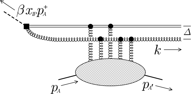
FIG. 1.: Structure of the diffractive gluon distribution. The top part is treated perturbatively. Any number of soft gluons are exchanged with the hadron matrix element represented on the bottom.

At large $1/x_{\scriptscriptstyle\kern-0.50003ptI\kern-1.25ptP}$ an eikonal approximation applies. There is a wave function $\psi$, describing the state of the fast moving gluon as it reaches the proton. This gluon passes through the proton at transverse position ${\bf\Delta}$ while the eikonal operator in Eq. (1) is located at transverse position ${\bf 0}$. The result, taken after a little manipulation from Eq. (3.38) of Ref. [2], is

$${\cal G}^{js} \approx {-1\over N_{c}^{2}-1}\ \int{dp_{\!A^{\prime}}^{+}\over(2\pi)2p_{A}^{+}}\ \int{d^{2}{\bf\Delta}\over{\bf\Delta}^{2}}\,\int{d^{2}\mbox{\boldmath$\ell$}\over(2\pi)^{2}}\,e^{-i\mbox{\boldmath$\ell$}\cdot{\bf\Delta}}\,{\partial\over\partial\ell^{i}}{\partial\over\partial\ell^{i}}\psi^{js}(\beta,{\bf k},{\bf k}+\mbox{\boldmath$\ell$})$$ (5)

$$\times\langle p_{\!A^{\prime}},s_{\!A^{\prime}}|{\rm Tr}\left[1-F({\bf\Delta})F^{T}({\bf 0})\right]|p_{\!A},s_{\!A}\rangle\hskip 5.69046pt.$$

Here the operators $F$ are color octet eikonal line operators:

$$F({\bf z})={\cal P}\ \exp\left\{-ig\int_{-\infty}^{+\infty}dz^{-}{\cal A}_{a}^{+}(0,z^{-},{\bf z})\,t_{a}\right\}\hskip 5.69046pt.$$ (6)

The wave function for the gluon state is

$$\psi^{js}(\beta,{\bf k},{\bf p})={\beta{\bf k}^{2}\delta^{js}+2(1-\beta)p^{j}p^{s}\over\beta{\bf k}^{2}+(1-\beta){\bf p}^{2}}.$$ (7)

We choose here to differentiate $\psi$ twice with respect to $\ell$. This has the effect of eliminating apparent ultraviolet divergences from the integration over $\bf k$ in the formulas that follow. The derivatives with respect to $\ell$ are compensated by a factor $(-1/{\bf\Delta}^{2})$ multiplying the matrix element of the eikonal operators. The factor $1/{\bf\Delta}^{2}$ does not itself produce a short distance divergence because both the matrix element and its first derivative with respect to ${\bf\Delta}$ vanish at ${\bf\Delta}={\bf 0}$. See Sec. 4.1 of Ref. [2] for a discussion of the ultraviolet behavior in the minimal case of two gluon exchange; exchanging more gluons does not make the ultraviolet behavior worse.

Consider now the matrix element of the eikonal operators between the initial and final proton states. The initial state carries zero transverse momentum. Let $-{\bf q}$ be the transverse momentum carried by the final state (${\bf q}^{2}\approx-t$). We may first expand this state in terms of eigenstates of transverse position with transverse position $-{\bf b}$ as

$$\langle p_{\!A^{\prime}},s_{\!A^{\prime}}|=\langle p_{\!A^{\prime}}^{+},-{\bf q},s_{\!A^{\prime}}|=\int d^{2}{\bf b}\ e^{-i\,{\bf b}\cdot{\bf q}}\ {}_{x}\!\langle p_{\!A^{\prime}}^{+},-{\bf b},s_{A^{\prime}}|\hskip 5.69046pt,$$ (8)

where the subscript $x$ on a state vector denotes that it is a position eigenstate. We then apply a translation to put the proton at transverse position ${\bf 0}$ and let the eikonal operators be at transverse positions ${\bf b}$ and ${\bf b}+{\bf\Delta}$. Taking into account that the eikonal operators do not transfer any plus momentum, we define a non-perturbative function $\Xi$ as

$$(2\pi)\ 2p_{\!A}^{+}\ \delta(p_{\!A^{\prime}}^{+}-p_{\!A}^{+})\ \Xi({\bf b}+{\bf\Delta},{\bf b};s_{\!A^{\prime}},s_{\!A})$$ (9)

$$\hskip 8.5359pt={1\over{N_{c}^{2}-1}}\,{}_{x}\!\langle p_{\!A^{\prime}}^{+},{\bf 0},s_{\!A^{\prime}}|{\rm Tr}\left[1-F({\bf b}+{\bf\Delta})F^{T}({\bf b})\right]|p_{\!A}^{+},{\bf 0},s_{\!A}\rangle\hskip 5.69046pt.$$ (10)

We use Eqs. (8) and (9) in Eqs. (2) and (5) to give

$${{d\,f_{g/A}^{\rm{diff}}(\beta,x_{\scriptscriptstyle\kern-0.50003ptI\kern-1.25ptP},t,\mu)}\over{dx_{\scriptscriptstyle\kern-0.50003ptI\kern-1.25ptP}\,dt}}=\int{d^{2}{\bf\Delta}\over{\bf\Delta}^{2}}\,{d^{2}{\bf\Delta}^{\prime}\over{{\bf\Delta}^{\prime}}^{2}}\,d^{2}{\bf b}\,d^{2}{\bf b}^{\prime}\,e^{-i\,({\bf b}-{\bf b}^{\prime})\cdot{\bf q}}\ {\cal I}(x_{\scriptscriptstyle\kern-0.50003ptI\kern-1.25ptP},\beta,{\bf\Delta},{\bf\Delta}^{\prime})$$ (12)

$$\times{1\over 2}\sum_{s_{\!A},s_{\!A^{\prime}}}\Xi^{*}({\bf b}^{\prime}+{\bf\Delta}^{\prime},{\bf b}^{\prime};s_{\!A^{\prime}},s_{\!A})\,\Xi({\bf b}+{\bf\Delta},{\bf b};s_{\!A^{\prime}},s_{\!A})$$

where

$${\cal I}(x_{\scriptscriptstyle\kern-0.50003ptI\kern-1.25ptP},\beta,{\bf\Delta},{\bf\Delta}^{\prime})={1\over{16\,\pi^{3}}}\,{N_{c}^{2}-1\over\beta(1-\beta)x_{\scriptscriptstyle\kern-0.50003ptI\kern-1.25ptP}^{2}}\int{d^{2}{\bf k}\over(2\pi)^{2}}\,\int{d^{2}{\mbox{\boldmath$\ell$}}\over(2\pi)^{2}}\,e^{-i{\mbox{\boldmath$\ell$}}\cdot{\bf\Delta}}\int{d^{2}{\mbox{\boldmath$\ell$}}^{\prime}\over(2\pi)^{2}}\ e^{i{\mbox{\boldmath$\ell$}}^{\prime}\cdot{\bf\Delta}^{\prime}}\$$ (13)

$$\times\left[{\partial\over\partial{\ell^{\prime}}^{k}}{\partial\over\partial{\ell^{\prime}}^{k}}\,\psi^{js}(\beta,{\bf k},{\bf k}+\mbox{\boldmath$\ell$}^{\prime})\right]^{*}\,\left[{\partial\over\partial\ell^{i}}{\partial\over\partial\ell^{i}}\,\psi^{js}(\beta,{\bf k},{\bf k}+\mbox{\boldmath$\ell$})\right]\hskip 5.69046pt.$$ (14)

Eq. (12) provides a representation for the diffractive gluon distribution in a physically appealing form. The $\beta$ dependence is entirely contained in the factor ${\cal I}$, which is constructed from the perturbative wave functions $\psi$. There are integrals over the global impact parameter of the collision (${\bf b}$ for the amplitude and ${\bf b}^{\prime}$ for the complex conjugate). The factor $\cal I$ does not depend on ${\bf b}$ or ${\bf b}^{\prime}$; these parameters merely tell where the proton is relative to the incoming partons. There are also integrals over the parton transverse separation (${\bf\Delta}$ for the amplitude and ${\bf\Delta}^{\prime}$ for its complex conjugate). The perturbative function ${\cal I}/({\bf\Delta}^{2}\,{{\bf\Delta}^{\prime}}^{2})$ gives the amplitudes for the partons to have separations ${\bf\Delta}$ and ${\bf\Delta}^{\prime}$; then the functions $\Xi$ describe the effect of the proton’s soft color field.

If we integrate the diffractive gluon distribution (12) over $x_{\scriptscriptstyle\kern-0.50003ptI\kern-1.25ptP}$ at fixed $x$ (or equivalently over $\beta$), this integration produces a logarithmic divergence coming from the region $\beta=x/x_{\scriptscriptstyle\kern-0.50003ptI\kern-1.25ptP}\ll 1$. In the case of the quark distribution there is no such divergence [2]. Then by integrating over $\beta$ one obtains a formula with only one separation parameter ${\bf\Delta}$. Formulas of this kind are given, e.g., in Refs. [4, 9, 11]. For the discussion that follows we are interested in the full $\beta$ spectrum, for which formulas with two separation parameters, ${\bf\Delta}$ and ${\bf\Delta}^{\prime}$, apply.

If we integrate the diffractive gluon distribution (12) over $t=-{\bf q}^{2}$ we obtain

$${{d\,f_{g/A}^{\rm{diff}}(\beta,x_{\scriptscriptstyle\kern-0.50003ptI\kern-1.25ptP},\mu)}\over{dx_{\scriptscriptstyle\kern-0.50003ptI\kern-1.25ptP}}}=4\pi\int{d^{2}{\bf\Delta}\over{\bf\Delta}^{2}}\,{d^{2}{\bf\Delta}^{\prime}\over{{\bf\Delta}^{\prime}}^{2}}\,d^{2}{\bf b}\ {\cal I}(x_{\scriptscriptstyle\kern-0.50003ptI\kern-1.25ptP},\beta,{\bf\Delta},{\bf\Delta}^{\prime})$$ (16)

$$\times{1\over 2}\sum_{s_{\!A},s_{\!A^{\prime}}}\Xi^{*}({\bf b}+{\bf\Delta}^{\prime},{\bf b};s_{\!A^{\prime}},s_{\!A})\,\Xi({\bf b}+{\bf\Delta},{\bf b};s_{\!A^{\prime}},s_{\!A}).$$

Now there is only one impact parameter, $\bf b$, but there are still two parton separation variables, ${\bf\Delta}$ and ${\bf\Delta}^{\prime}$.

We now turn to the hadronic matrix element $\Xi$. If, as in Ref. [12], the proton were replaced by a small meson made of heavy quarks, then perturbation theory would be applicable to compute $\Xi$. But for a large state, such as a proton, we need to rely on a combination of perturbative and nonperturbative ideas to construct an approximation for $\Xi$.

We first recognize that $\Xi$ is an absorption amplitude. Imagine that two high momentum gluons, represented by eikonal operators, impinge upon the proton at transverse positions ${\bf b}$ and ${\bf b}+{\bf\Delta}$. Suppose that the gluons completely miss the proton. Then each of the two operators $F$ in $1-F({\bf\Delta})F^{T}({\bf 0})$ can be replaced by unit operators so that $\Xi=0$. Now, suppose that one or both of ${\bf b}$ and ${\bf b}+{\bf\Delta}$ is inside the proton, with no particular relation between these positions. Then we expect that the amplitude for the proton to remain a ground state proton after the passage of the gluon(s) is approximately zero, $\langle p|F\,F^{T}|p\rangle\approx 0$, so that $\Xi\approx 1\times\delta_{s_{A}s_{A^{\prime}}}$. Thus a simple model for $\Xi$ might be

$${\cal A}({\bf b}+{\bf\Delta},{\bf b})\ \delta_{s_{A}s_{A^{\prime}}}$$ (17)

where $\cal A$ is a smooth function such that ${\cal A}\approx 0$ if $|{\bf b}+{\bf\Delta}|\gg R_{p}^{2}$ and $|{\bf b}|\gg R_{p}^{2}$ and ${\cal A}\approx 1$ if either $|{\bf b}+{\bf\Delta}|\ll R_{p}^{2}$ or $|{\bf b}|\ll R_{p}^{2}$, where $R_{p}$ is the radius of the proton.

An important exception arises if ${\bf\Delta}$ is small. Then $F({\bf b})^{T}$ is nearly the inverse of $F({\bf b}+{\bf\Delta})$, so that $\Xi\approx 0$. To take this color transparency effect into account, we modify our model to

$${\cal A}({\bf b}+{\bf\Delta},{\bf b})\ \delta_{s_{A}s_{A^{\prime}}}\,[1-\exp(-\kappa_{g}^{2}{\bf\Delta}^{2}/2)].$$ (18)

Then $\Xi\approx 0$ for small $\bf\Delta$ but for large $\bf\Delta$ we retain the absorption physics explained above. Here $1/\kappa_{g}$ is a parameter that measures how close together the gluons have to be before they can traverse the proton without breaking it up. That is, $1/\kappa_{g}$ is the largest size for a color octet dipole for which the proton is transparent. We hypothesize that $1/\kappa_{g}$ is small: $1/\kappa_{g}\ll R_{p}.$

In Eq. (18) we have chosen a gaussian function for reasons of simplicity. Any function that vanishes for $\kappa_{g}{\bf\Delta}\ll 1$ and tends to 1 for $\kappa_{g}{\bf\Delta}\gg 1$ could be used in place of $[1-\exp(-\kappa_{g}^{2}{\bf\Delta}^{2}/2)]$.

We now note that the function $\cal I$ is singular when ${\bf\Delta}$ and ${\bf\Delta}^{\prime}$ become small. In fact, straightforward dimensional analysis shows that for $|{\bf\Delta}|\sim|{\bf\Delta}^{\prime}|$, ${\cal I}\sim{\mbox{const.}}/(|{\bf\Delta}|\,|{\bf\Delta}^{\prime}|)$. For this reason, the important contributions to the integral over ${\bf\Delta}$ comes from small ${\bf\Delta}$, $|{\bf\Delta}|\sim 1/\kappa_{g}\ll R_{p}$. In this circumstance, we can set ${\bf\Delta}$ to zero in ${\cal A}({\bf b}+{\bf\Delta},{\bf b})$, giving

$$\Xi({\bf b}+{\bf\Delta},{\bf b};s_{\!A^{\prime}},s_{\!A})={\cal A}({\bf b},{\bf b})\,\delta_{s_{A}s_{A^{\prime}}}\,[1-\exp(-\kappa_{g}^{2}{\bf\Delta}^{2}/2)].$$ (19)

This is our model. The proton can survive, $\Xi\approx 0$, if either ${\bf b}$ is large or ${\bf\Delta}$ is small. The model incorporates saturation [3, 4, 11]: as $|{\bf\Delta}|$ increases, the absorption amplitude increases, but it never gets to be larger than 1. Furthermore, the important transverse separations are small [2, 3, 4, 11].

We now use Eq. (19) in Eq. (16). The integral in ${\bf b}$ over the absorption function $\cal A$ must give a quantity of order $R_{p}^{2}$:

$$\int d^{2}{\bf b}\ |{\cal A}({\bf b},{\bf b})|^{2}=\lambda_{\cal A}\ R_{p}^{2}\hskip 5.69046pt,$$ (20)

where the precise coefficient $\lambda_{\cal A}$ depends on the detailed form of the function $\cal A$. In the numerical evaluations that follow we take $R_{p}$ to be the charge radius of the proton, $R_{p}=0.88\ {\rm fm}$ [13], and we take $\lambda_{\cal A}=1$. Using Eq. (20) and Eq. (13) for ${\cal I}$ in Eq. (16), we see that

$${{d\,f_{g/A}^{\rm{diff}}}\over{dx_{\scriptscriptstyle\kern-0.50003ptI\kern-1.25ptP}}}={{(N_{c}^{2}-1)\,\lambda_{\cal A}\ R_{p}^{2}\ \kappa_{g}^{2}}\over x_{\scriptscriptstyle\kern-0.50003ptI\kern-1.25ptP}^{2}}\ g(\beta)\hskip 5.69046pt,$$ (21)

where $g(\beta)$ is a function of $\beta$ that we determine by calculating the integrals numerically in a suitable momentum space representation. The behavior in $\kappa_{g}$ is perhaps surprising – the larger $\kappa_{g}$, the larger the cross section. But it reflects an essential feature of the diffraction process: because of the singular nature of the wave functions the amplitude is dominated by distances of order $1/\kappa_{g}$.

Notice that the result (21) has an $x_{\scriptscriptstyle\kern-0.50003ptI\kern-1.25ptP}$ dependence $x_{\scriptscriptstyle\kern-0.50003ptI\kern-1.25ptP}^{-2}$. This results from our simple treatment of the soft exchanged gluons, which we treat as having rapidities near zero in the proton rest frame. In a more sophisticated treatment, one would have a BFKL ladder of exchanged gluons with rapidities becoming large and negative along the ladder. This would lead to a dependence $x_{\scriptscriptstyle\kern-0.50003ptI\kern-1.25ptP}^{-2-2\delta}$ with $\delta$ proportional to $\alpha_{s}$. We do not pursue such a treatment here. However, in order to compare with experimental data, we suppose that the simple treatment is approximately correct for $x_{\scriptscriptstyle\kern-0.50003ptI\kern-1.25ptP}$ of order $x_{0}$, where $x_{0}$ is small but not too small, and that there are corrections for $x_{\scriptscriptstyle\kern-0.50003ptI\kern-1.25ptP}\ll x_{0}$. Thus we multiply our result by $x_{0}^{2\delta}/x^{2\delta}$. We use the experimental value $\delta=0.15$ [14, 15] and take $x_{0}=0.01$. This gives

$${{d\,f_{g/A}^{\rm{diff}}}\over{dx_{\scriptscriptstyle\kern-0.50003ptI\kern-1.25ptP}}}={{(N_{c}^{2}-1)\,x_{0}^{2\delta}\,\lambda_{\cal A}\,\ R_{p}^{2}\ \kappa_{g}^{2}}\over x_{\scriptscriptstyle\kern-0.50003ptI\kern-1.25ptP}^{2+2\delta}}\ g(\beta)\hskip 5.69046pt.$$ (22)

A treatment analogous to that described for the gluon may now be applied to the quark distribution, using the appropriate quark operators as described in [2]. Similarly to Eq. (21), the answer has the form

$${{d\,f_{q/A}^{\rm{diff}}}\over{dx_{\scriptscriptstyle\kern-0.50003ptI\kern-1.25ptP}}}={{N_{c}\,x_{0}^{2\delta}\,\lambda_{\cal A}\,R_{p}^{2}\,\kappa_{q}^{2}}\over x_{\scriptscriptstyle\kern-0.50003ptI\kern-1.25ptP}^{2+2\delta}}\ q(\beta)\hskip 5.69046pt.$$ (23)

The function $q(\beta)$ is different than in the gluon case due to the different lightcone wave functions $\psi$. The color factor is different. Finally, the scale $\kappa_{q}$ is different because color triplet eikonal operators now replace color octet operators in the functions $\Xi$. From the color structure of these operators, we expect $\kappa_{g}$ and $\kappa_{q}$ to be roughly in the relation $\kappa_{g}/\kappa_{q}\approx C_{A}/C_{F}$. Note that, together with the color factors explicitly shown in Eqs. (22) and (23), this gives back the factor $C_{A}^{2}(N_{c}^{2}-1)/(C_{F}^{2}N_{c})=27/2$ of Ref. [2] in the ratio between the gluon and the quark distributions. Note also that, since $\kappa_{q}<\kappa_{g}$, the typical separation ${\bf\Delta}$ in the case of quarks will be larger than in the case of gluons, so that the perturbative evaluation that we have used may be less reliable in the quark case.

The treatment discussed so far does not contain scaling violation. Having worked in a short-distance factorization framework, we may include the graphs that give scaling violation systematically by using next-to-leading-order hard scattering coefficients and DGLAP evolution equations, as in Ref. [2]. We then compute predictions for the diffractive structure function $F_{2}^{\rm{diff}}$.

What, then, should be the starting scale $\mu_{0}$ for evolution? Evidently, $\mu_{0}$ should be roughly comparable to the physical scales $\kappa_{g}$ and $\kappa_{q}$. To go further, consider the term $P_{qg}\otimes f_{g}$ in the evolution equation for the diffractive quark distribution at scale $\mu_{0}$. The quark and antiquark have a transverse separation of order $1/\mu_{0}$. The quark-antiquark system is separated from the gluon by a larger distance, which, for us, is of order $1/\kappa_{g}$. Thus $1/\mu_{0}$ should be somewhat smaller than $1/\kappa_{g}$.

FIG. 2.: The data for $F_{2}^{\rm{diff}}$ from Ref. [15] compared with the theory results described in the text for two different sets of scale parameters.

Our results for $F_{2}^{\rm{diff}}$ depend on $\kappa_{g}$, $\kappa_{q}$, and $\mu_{0}$. Approximate values for these scales may be extracted by comparing the predictions with experiment. Note that a very precise determination is difficult because of the uncertainty in the normalization of the model, which arises from the uncertainty in the factors $\lambda_{\cal A}$ and $x_{0}^{2\delta}$ in Eqs. (22) and (23). This normalization uncertainty affects the determination of $\kappa_{q}$ directly. The parameter $\mu_{0}$ and the ratio $\kappa_{q}/\kappa_{g}$ influence the shape of $F_{2}^{\rm diff}$ in $\beta$ and $Q^{2}$, so their determination is less directly affected.

In Fig. 2 we compare the results for $F_{2}^{\rm{diff}}$ with the data of Ref. [15] by plotting data minus theory over theory, where the theory in the two plots is the one corresponding to the two displayed sets of values for $1/\mu_{0}$, $1/\kappa_{g}$, $1/\kappa_{q}$. Recall that, for the self-consistency of the physical picture that we have discussed, we expect these distance scales to be small compared to $R_{p}$. For the case of Fig. 2a, we find that the agreement between theory and data is reasonable, given the simplicity of the model. The size $1/\mu_{0}$ of the quark-antiquark pair here is smallest and the ratio $\kappa_{g}/\kappa_{q}$ of the sizes of the color-triplet to the color-octet systems comes out to be in rough agreement with the expectation $C_{A}/C_{F}$ mentioned above. In Fig. 2b we increase the value of $1/\mu_{0}$ and then adjust $1/\kappa_{g}$ and $1/\kappa_{q}$ so as to describe the data as well as possible. We observe that the data seem to disfavor these larger distance scales: the shape of the data, in particular, is not well reproduced in this case.

It is now worth looking back at Fig. 1 and the structure of Eq. (16). The function $\Xi$, representing the lower part of Fig. 1 and including the exchange of any number of soft gluons, is nonperturbative. We have posited a description for $\Xi$ in terms of an absorption function and a color transparency factor. The upper part of Fig. 1 is also, in general, nonperturbative, because it still contains arbitrarily large parton separations $|{\bf\Delta}|$. Indeed, in the upper part of Fig. 1 one would expect to have not just two but several fast partons impinging on the proton, each with a large transverse separation with respect to the others. But if the separations are large, then absorption dominates the hadronic matrix element, so that central collisions are unlikely to leave the proton intact. Thus, the parton transverse separations must be smaller than the color transparency scale. If this scale is small enough, a perturbation expansion for the upper part of Fig. 1 is justified. At lowest perturbative order there are only two partons (including the eikonal line) and we obtain the calculated function $\cal I$. At higher perturbative orders there can be multiple partons, all close together; these are the configurations that we include through radiative corrections to the hard scattering and evolution.

The results of Fig. 2 provide a justification for this expansion and lend support to the physical picture of diffractive DIS as being due to color-dipole parton systems penetrating the proton at small transverse separations. In particular, a partonic system in a configuration of a color octet dipole, which corresponds to the diffractive gluon distribution, must be especially small in transverse size. This contributes to the diffractive gluon distribution being especially large, as is consistent with the data. The picture described in this paper provides a concrete model for the mechanism through which the dominance of small size states [2, 12] may be realized in diffractive DIS at HERA. More and better data will be valuable to investigate this further and decide whether or not the indications of Fig. 2 are confirmed.

We gratefully acknowledge discussions with J. Collins, M. Diehl, Z. Kunszt, A. Mueller, G. Sterman and M. Strikman. Our work is supported in part by the US Department of Energy under grants DE-FG02-90ER40577 and DE-FG03-96ER40969. F.H. acknowledges the hospitality of the University of Oregon while part of this work was being done.

REFERENCES

- [1] H. Abramowicz, hep-ph/0001054, contributed to the 19th International Symposium on Lepton and Photon Interactions at High Energies, Stanford University, August 1999.
- [2] F. Hautmann, Z. Kunszt and D.E. Soper, Nucl. Phys. B563, 153 (1999).
- [3] A.H. Mueller, in Proceedings of the International Workshop on Deep Inelastic Scattering DIS98, Brussels, Belgium, 1998, edited by G. Coremans and R. Roosen (World Scientific, Singapore, 1998), p.3; Nucl. Phys. B558, 285 (1999).
- [4] K. Golec-Biernat and M. Wüsthoff, Phys. Rev. D 60, 114023 (1999).
- [5] E. Gotsman, E. Levin and U. Maor, Nucl. Phys. B493, 354 (1997).
- [6] L. Frankfurt and M. Strikman, Nucl. Phys. B Proc. Suppl. 79, 671 (1999) (hep-ph/9907221); M. McDermott, L. Frankfurt, V. Guzey and M. Strikman, hep-ph/9912547.
- [7] H1 Collaboration, paper 960 submitted to ICHEP2000, Osaka, Japan, July 2000; M. Martinez, talk 02c-03 at ICHEP2000.
- [8] J.D. Bjorken, AIP Conference Proceedings No. 6, Particles and Fields subseries No. 2 (New York 1972); hep-ph/9601363; J.D. Bjorken, J. Kogut and D.E. Soper, Phys. Rev. D 3, 1382 (1971).
- [9] N.N. Nikolaev and B.G. Zakharov, Z. Phys. C 49, 607 (1991); 53, 331 (1992).
- [10] J. Bartels, J. Ellis, H. Kowalski and M. Wüsthoff, Eur. Phys. J. C7, 443 (1999).
- [11] A. Hebecker, Phys. Rept. 331, 1 (2000); W. Buchmüller, T. Gehrmann and A. Hebecker, Nucl. Phys. B537, 477 (1999); A. Hebecker and H. Weigert, Phys. Lett. B 432, 215 (1998).
- [12] F. Hautmann, Z. Kunszt and D.E. Soper, Phys. Rev. Lett. 81, 3333 (1998); hep-ph/9905218.
- [13] R. Rosenfelder, Phys. Lett. B 479, 381 (2000); K. Melnikov and T. van Ritbergen, Phys. Rev. Lett. 84, 1673 (2000).
- [14] H1 Collaboration, (C. Adloff et al.), Z. Phys. C 76, 613 (1997).
- [15] ZEUS Collaboration (J. Breitweg et al.), Eur. Phys. J. C6, 43 (1999).