Active-Sterile Neutrino Transformation
and r-Process Nucleosynthesis

Abstract

The type II supernova is considered as a candidate site for the production of heavy elements. Since the supernova produces an intense neutrino flux, neutrino scattering processes will impact element formation. We examine active-sterile neutrino conversion in this environment and find that it may help to produce the requisite neutron-to-seed ratio for synthesis of the r-process elements.

The r-process of nucleosynthesis accounts for the most neutron rich of the heavy elements. The most likely environment for this type of synthesis is the late time ($t>10\,{\rm s}$ post-core bounce) supernova environment. Many studies have explored this ‘neutrino driven wind’ as a candidate environment and found it to be potentially viable r1 ; me92 . However, to date, no model correctly reproduces the observed abundance pattern.

In the neutrino driven wind, material in the form of free nucleons is ‘lifted’ off of the surface of the neutron star by energy deposited by neutrino interactions. Analytic and semianalytic parameterizations of the thermodynamic and hydrodynamic conditions in the wind can be obtained dun ; qw . Models of this type may be used to explore the range of conditions within the context of the wind which will produce the solar system distribution of r-process elements. The key determinant of whether a given scenario will produce the r-process is the neutron to seed nucleus ratio at the onset of the neutron capture phase. This ratio must be quite high ($R>100$) in order to produce the very neutron-rich r-process elements. The factors which determine the neutron-to-seed ratio are the entropy of the material, the hydrodynamic outflow timescale and the electron fraction, $Y_{e}=1/(1+n/p)$ where $n/p$ is the neutron-to-proton ratio. A study of many possible model parameters shows that one must decrease the electron fraction, and/or increase the entropy and/or decrease the hydrodynamic outflow timescale, relative to the conditions found in typical wind models, in order to produce the neutron-to-seed ratio necessary for the r-process me97 ; hwq .

Including the effects of neutrino interactions in general tends to make the requisite conditions for r-process element production more extreme me95 ; fm95 . In particular, neutrino capture on free nucleons during alpha particle formation increases the electron fraction fm95 . This is the “alpha effect”. Other neutrino process are discussed in me92 ; wick .

There are three possible solutions to this problem. The first is that the supernova is the site of r-process synthesis, but it does not occur in the neutrino driven wind as it is currently modeled. The second is that the r-process elements are made at some other site such as neutron star-neutron star mergers. However, timescale arguments combined with isotopic abundance measurements and observations of old halo star metallicity show that this site is unlikely to account for the entire r-process distribution wasserburg ; sneden .

The third solution is the one that is investigated here: active-sterile ($\nu_{e}\leftrightarrow\nu_{s}$, $\bar{\nu_{e}}\leftrightarrow\bar{\nu_{s}}$) neutrino transformation. The $\nu_{s}$ in our study is defined as a particle which mixes with the $\nu_{e}$ (and possibly also with $\nu_{\mu}$, and/or $\nu_{\tau}$) but does not contribute to the width of the Z boson.

If we neglect $\nu$-$\nu$ forward scattering contributions to the weak potentials, then the equation which governs the evolution of the neutrinos as they pass though the material in the wind can be written as:

$$i\hbar\frac{\partial}{\partial r}\left[\begin{array}[]{cc}\Psi_{e}(r)\\ \\ \Psi_{s}(r)\end{array}\right]=\left[\begin{array}[]{cc}\varphi_{e}(r)&(\delta m^{2}/4E)\sin{2\theta_{v}}\\ \\ (\delta m^{2}/4E)\sin{2\theta_{v}}&-\varphi_{e}(r)\end{array}\right]\left[\begin{array}[]{cc}\Psi_{e}(r)\\ \\ \Psi_{s}(r)\end{array}\right]\,,$$ (1)

where

$$\varphi_{e}(r)=\frac{1}{4E}\left(\pm 2\sqrt{2}\ G_{F}\left[N_{e}^{-}(r)-N_{e}^{+}(r)-\frac{N_{n}(r)}{2}\right]E-\delta m^{2}\cos{2\theta_{v}}\right)$$ (2)

The upper sign is relevant for neutrino transformations; the lower one is for antineutrinos. In these equations $\delta m^{2}\equiv m_{2}^{2}-m_{1}^{2}$ is the vacuum mass-squared splitting, $\theta_{v}$ is the vacuum mixing angle, $G_{F}$ is the Fermi constant, and $N_{e}^{-}(r)$, $N_{e}^{+}(r)$, and $N_{n}(r)$ are the total proper number densities of electrons, positrons, and neutrons respectively in the medium. Resonances can occur when the on-diagonal terms in the wave equation are zero. The quantity in the brackets in Eq. 2 is proportional to $Y_{e}-1/3$. Since the electron fraction can take on values between zero and one, the bracketed quantity in Eq. 2 can be either positive or negative. Therefore, for a given choice of $\delta m^{2}$, resonances may occur for neutrinos or antineutrinos depending on the value of the electron fraction.

In order to determine the survival probabilities of the neutrinos and antineutrinos, we must know the electron fraction. In the neutrino driven wind, neutrino and antineutrino capture are the most important reactions in determining the electron fraction. However, near the surface of the protoneutron star there is also a contribution from electrons and positrons:

$$\nu_{e}+{\rm n}\rightleftharpoons{\rm p}+e^{-};\;\;\;\bar{\nu}_{e}+{\rm p}\rightleftharpoons{\rm n}+e^{+}.$$ (3)

Therefore, the problem involves a feedback mechanism. The neutrino capture rates determine the electron fraction and the electron fraction determines the potential which is used in the neutrino transformation equations. These equations then determine survival probabilities of the neutrinos, and therefore their capture rates.

We note that we can not assume weak equilibrium, (very fast capture rates compared with outflow rate) or weak freeze-out (very slow rates compared with the outflow rate). The rates must be tracked numerically. A previous study took the limit of weak equilibrium and found different behavior nunokawa than presented here.

We perform calculations by tracking a mass element in the neutrino driven wind. We use the results of analytic models qw , where $r\propto\exp(-t/\tau)$ and $\rho\propto r^{-3}$ where $\tau$ is the outflow timescale. Close to the surface, before the wind begins to operate we use the density profile of Wilson and Mayle wilson . At each time step we calculate all thermodynamic quantities, calculate the weak rates and evolve the neutrino transformation equations forward. We assume, since the outflow timescale is short, $t\sim\tau\lesssim 0.5\,{\rm s}$, that each mass element will have the same evolution as the previous one. Since we use a nuclear statistical equilibrium calculation, we cut our calculations off at the time when heavy nuclei begin to form. More detail is contained in us .

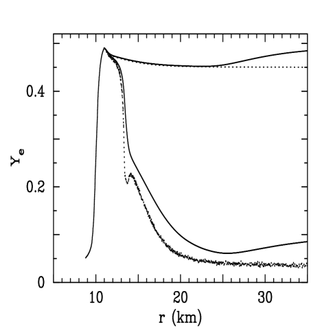
Figure 1: The electron fraction is plotted against distance from the center of the neutron star. The upper line shows the evolution with no transformation. The lower line shows the evolution of active-sterile mixing parameters of $\sin^{2}\theta=0.01$ and $\delta m^{2}=20\,{\rm eV}^{2}$. The dotted line shows the value that the electron fraction would take on if weak equilibrium obtained.

A calculation for one mass element is shown in Fig. 1. The upper curve shows the evolution for the case of no neutrino oscillations. The wind parameters were $\tau=0.3\,{\rm s}$, $s=100$. The solid line shows the actual electron fraction, while the dotted line shows what the electron fraction would be if weak equilibrium obtained. The initial rise is due to Pauli unblocking of the electrons at the surface of the proto-neutron star. The lower curve shows the evolution of the electron fraction for mixing parameters of $\delta m^{2}=20\,{\rm eV}^{2}$, $\sin^{2}2\theta_{\rm v}=0.01$. In the latter case there is a rapid drop in the electron fraction when the neutrinos begin to transform. In fact, there are three neutrino transformations. Initially, the electron neutrinos transform to steriles. Later antineutrinos transform, and finally, when the density falls far enough the antineutrinos transform back. The first transformation of the antineutrinos is seen in the small bump in the equilibrium electron fraction. A small “alpha effect” can be see as the slight rise in both solid lines at large distance.

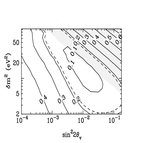
Figure 2: Contour plot of electron fraction as measured at the point where heavy nuclei begin to form. Neutrino driven wind parameters employed here are $s/k=100$, $\tau=0.3{\rm s}$. .

The active-sterile transformation scenario successfully reproduces a low electron fraction which is beneficial to the r-process. We now consider a range of $\delta m^{2}$, $\sin^{2}\theta$ parameters. A contour plot of the electron fraction is shown in Fig. 2. Inside the dashed contour shows the region where conditions are neutron-rich enough to be favorable for r-process nucleosynthesis. In the bottom left corner of the plot, the solution is approaching the case without neutrino transformation.

Although not shown here, we have studied a range of timescales for the neutrino driven wind models, and seen that the qualitative features of this effect are reproduced us .

We have used several approximations in our calculations, which we are continuing to study. These include the importance of the neutrino-neutrino scattering background in the oscillation equations, the importance of nonradial paths and feedback in the dense region near the proto-neutron star. The region where the latter two are important is the shaded region in Fig. 2. These problems are being studied in us2 .

Conclusions: Meteoritic and observational evidence points to supernovae as the source of the r-process elements, although a self-consistent model of the neutrino driven wind which will produce the r-process elements is still elusive. In the next few years significant advances are expected in supernova modeling. If and when potential hydrodynamic solutions are exhausted and the caveats above have been explored, then the r-process may provide a signature for new neutrino physics.

References

- (1) Woosley, S. E., Wilson, J. R., Mathews, G. J., Hoffman, R. D. and Meyer, B. S. Astrophys. J. 433, 229-246 (1994), Takahashi, K., Witti, J., and Janka, H.-Th Astron. Astrophys. 286, 857-869 (1994).
- (2) Meyer, B. S., Howard, W. M. Mathews, G. J., Woosley, S. E., and Hoffman, R. D. Astrophys. J. 399, 656-664 (1992).
- (3) Duncan, R. C., Shapiro, S. L., & Wasserman, I. Astrophys. J., 309, 141-160 (1986).
- (4) Qian, Y.-Z. and Woosley, S. E. Astrophys. J., 471, 331-351 (1996).
- (5) Meyer, B. S. and Brown, J. S. Astrophys. J. Suppl. 112, 199-220, (1997).
- (6) Hoffman, R. D., Woosley, S. E. and Qian, Y.-Z.Astrophys. J. 482, 951-962 (1997).
- (7) Meyer, B. S. Astrophys J., 449, L55-L58 (1995)
- (8) Fuller, G. M., and Meyer, B. S., it Astrophys J., 453, 792-809, (1995), McLaughlin, G. C., Fuller, G. M. and Wilson, J. R., it Astrophys J., 472, 440-451, (1996), Meyer, B. S., McLaughlin, G. C. and Fuller, G. M., Phys. Rev. C, 59 2873-2887 (1998).
- (9) Haxton, et. al., Phys. Rev.Lett. 78, 2694-2697 (1997)
- (10) Qian, Y.-Z. and Wasserburg, G. J., Phys. Rept. 333-334, 77-108 (2000)
- (11) Sneden C. et al., Astrophys. J., 467, 819-840, (1996), Sneden, C. et al. Astrophys. J., 496, 235-245, (1998).
- (12) Nunokawa, H., Rossi, A., Semikoz, V. and Valle, J. W. F. Phys. Rev. D56 1704-1713 (1997).
- (13) Mayle, R. W. and Wilson, J. R., unpublished (1993).
- (14) McLaughlin, G. C., Fetter, J. M., Balantekin, A. B. and Fuller, G. M., Phys. Rev. C59, 2873-2887. (1999)
- (15) Fetter, J. M., Balantekin, A. B. and Fuller, G. M., and McLaughlin, G. C. in preparation (2000).