CERN–TH/2000-244

hep-ph/0008184

Universality of non-leading logarithmic contributions
in transverse-momentum distributions

Stefano Catani^(a) , Daniel de Florian^(b)   and   Massimiliano Grazzini^(b) 

^(a)Theory Division, CERN, CH 1211 Geneva 23, Switzerland

^(b)Institute for Theoretical Physics, ETH-Hönggerberg, CH 8093 Zürich, Switzerland

Abstract

We consider the resummation of the logarithmic contributions to the region of small transverse momenta in the distributions of high-mass systems (lepton pairs, vector bosons, Higgs particles, $\dots$) produced in hadron collisions. We point out that the resummation formulae that are usually used to compute the distributions in perturbative QCD involve process-dependent form factors and coefficient functions. We present a new universal form of the resummed distribution, in which the dependence on the process is embodied in a single perturbative factor. The new form simplifies the calculation of non-leading logarithms at higher perturbative orders. It can also be useful to systematically implement process-independent non-perturbative effects in transverse-momentum distributions. We also comment on the dependence of these distributions on the factorization and renormalization scales.

CERN–TH/2000-244

August 2000

The properties of the transverse-momentum distributions of systems of high mass $Q$ produced at high-energy hadron colliders are important for QCD studies and for physics studies beyond the Standard Model (see, e.g., Refs. [1]–[3]). On the theoretical side the computation of these distributions is complicated by the presence of large logarithmic contributions of the type $\ln Q^{2}/q_{\perp}^{2}$, which spoil the convergence of fixed-order perturbative calculations in the region of small transverse momenta $q_{\perp}$. The logarithmically-enhanced terms have to be evaluated at higher perturbative orders, and possibly resummed to all orders in the QCD coupling $\alpha_{\mathrm{S}}$. The all-order resummation formalism was developed in the eighties [4]–[12]. The structure of the resummed distribution is given in terms of a transverse-momentum form factor and of process-dependent contributions.

The transverse-momentum form factor is sometimes supposed to be universal, that is, independent of the process. Performing a process-independent calculation at relative order $\alpha_{\mathrm{S}}^{2}$, two of us have recently shown [13] in an explicit way that the form factor depends on the process. In this note, we give a general interpretation of the results in Ref. [13]. We point out that this process-dependent features persist to higher orders, at least in the final form in which the resummed transverse-momentum distribution is usually organized. We also present a new form of the resummed distribution, where all the logarithmic contributions are embodied in universal (process-independent) factors.

We consider the inclusive hard-scattering process

$$h_{1}(p_{1})+h_{2}(p_{2})\rightarrow F(Q^{2},q_{\perp}^{2})+X\;\;,$$ (1)

where the triggered final-state system $F$ is produced by the collision of the two hadrons $h_{1}$ and $h_{2}$ with momenta $p_{1}$ and $p_{2}$, respectively. We denote by $\sqrt{s}$ the centre-of-mass energy of the colliding hadrons $(s=(p_{1}+p_{2})^{2}\simeq 2p_{1}p_{2})$. The final state $F$ is a generic system of non-strongly interacting particles , such as one or more vector bosons $(\gamma^{*},W,Z,\dots)$, Higgs particles ($H$) and so forth.

To simplify the discussion we limit ourselves to the case in which only the total invariant mass $Q$ and transverse momentum $q_{\perp}$ (with respect to the direction of the colliding hadrons) of the system $F$ are measured. The extension to more general kinematic configurations, in which, for instance, the rapidities are measured, is straightforward (see the discussion below Eq. (25)). We also assume that at the parton level the system $F$ is produced with vanishing $q_{\perp}$ (i.e. with no accompanying final-state radiation) in the leading-order (LO) approximation, so that the corresponding cross section is $d\sigma^{(LO)}/dq_{\perp}^{2}\propto\delta(q_{\perp}^{2})$. Since $F$ is colourless, the LO partonic subprocess is either $q{\bar{q}}$ annihilation, as in the case of $\gamma^{*},W$ and $Z$ production, or $gg$ fusion, as in the case of the production of a Higgs boson $H$.

The transverse-momentum cross section for the process in Eq. (1) can be written as [5, 8, 9]

$$\frac{d\sigma_{F}}{dQ^{2}\;dq_{\perp}^{2}}=\left[\frac{d\sigma_{F}}{dQ^{2}\;dq_{\perp}^{2}}\right]_{{\rm res.}}+\left[\frac{d\sigma_{F}}{dQ^{2}\;dq_{\perp}^{2}}\right]_{{\rm fin.}}\;\;.$$ (2)

Both terms on the right-hand side are obtained as convolutions of partonic cross sections and the parton distributions $f_{a/h}(x,Q^{2})$ ($a=q_{f},{\bar{q}}_{f},g$ is the parton label) of the colliding hadrons. The distinction between the two terms is purely theoretical. The partonic cross section that enters in the resummed part (the first term on the right-hand side) contains all the logarithmically-enhanced contributions $\alpha_{\mathrm{S}}^{n}\ln^{m}Q^{2}/q_{\perp}^{2}$. Thus, this part has to be evaluated by resumming the logarithmic terms to all orders in perturbation theory. On the contrary, the partonic cross section in the second term on the right-hand side is finite order-by-order in perturbation theory when $q_{\perp}\rightarrow 0$. It can thus be computed by truncating the perturbative expansion at a given fixed order in $\alpha_{\mathrm{S}}$.

The finite component of the transverse-momentum cross section is obviously process-dependent, and we have nothing to add on it in this paper. In the following we discuss the structure of the resummed part.

The resummed component is

$$\left[\frac{d\sigma_{F}}{dQ^{2}\;dq_{\perp}^{2}}\right]_{{\rm res.}} = \sum_{a,b}\int_{0}^{1}dx_{1}\int_{0}^{1}dx_{2}\int_{0}^{\infty}db\;\frac{b}{2}\;J_{0}(bq_{\perp})\;f_{a/h_{1}}(x_{1},b_{0}^{2}/b^{2})\;f_{b/h_{2}}(x_{2},b_{0}^{2}/b^{2})$$ (3)

$$\cdot W_{ab}^{F}(x_{1}x_{2}s;Q,b)\;\;.$$

The Bessel function $J_{0}(bq_{\perp})$ and the coefficient $b_{0}=2e^{-\gamma_{E}}$ ($\gamma_{E}=0.5772\dots$ is the Euler number) have a kinematical origin. To correctly take into account the kinematics constraint of transverse-momentum conservation, the resummation procedure has to be carried out in the impact-parameter space. The transverse-momentum cross section (3) is then obtained by performing the inverse Fourier (Bessel) transformation with respect to the impact parameter $b$. The factor $W_{ab}^{F}$ is the perturbative and process-dependent partonic cross section that embodies the all-order resummation of the large logarithms $\ln Q^{2}b^{2}$ (the limit $q_{\perp}\ll Q$ corresponds to $Qb\gg 1$, because $b$ is the variable conjugate to $q_{\perp}$).

The resummed partonic cross section is usually (see, e.g., the list of references in Sections 5.1 and 5.3 of Ref. [1]) written in the following form:

$$W_{ab}^{F}(s;Q,b) = \sum_{c}\int_{0}^{1}dz_{1}\int_{0}^{1}dz_{2}\;C_{ca}^{F}(\alpha_{\mathrm{S}}(b_{0}^{2}/b^{2}),z_{1})\;C_{{\bar{c}}b}^{F}(\alpha_{\mathrm{S}}(b_{0}^{2}/b^{2}),z_{2})\;\delta(Q^{2}-z_{1}z_{2}s)$$ (4)

$$\cdot \sigma_{c{\bar{c}}}^{(LO)\,F}(Q^{2})\;S_{c}^{F}(Q,b)\;\;.$$

Here, $\sigma_{c{\bar{c}}}^{(LO)\,F}$ is the cross section (integrated over $q_{\perp}$) for the LO partonic subprocess $c+{\bar{c}}\rightarrow F$, where $c,{\bar{c}}=q,{\bar{q}}$ (the quark $q_{f}$ and the antiquark ${\bar{q}}_{f^{\prime}}$ can possibly have different flavours $f,f^{\prime}$) or $c,{\bar{c}}=g,g$. The expression $\sigma_{c{\bar{c}}}^{(LO)\,F}$ can include an overall factor $\alpha_{\mathrm{S}}^{p}(Q^{2})$, as in the case of $g+g\rightarrow H$ through a triangular quark loop where $p=2$. The term $S_{c}^{F}(Q,b)$ is the quark $(c=q)$ or gluon $(c=g)$ Sudakov form factor. The resummation of the logarithmic contributions is achieved by exponentiation [4]–[7], that is by showing [8, 9] that the form factor can be expressed as

$$S_{c}(Q,b)=\exp\left\{-\int_{b_{0}^{2}/b^{2}}^{Q^{2}}\frac{dq^{2}}{q^{2}}\left[A_{c}(\alpha_{\mathrm{S}}(q^{2}))\;\ln\frac{Q^{2}}{q^{2}}+B_{c}(\alpha_{\mathrm{S}}(q^{2}))\right]\right\}\;\;,$$ (5)

with $c=q$ or $g$. The functions $A_{c}(\alpha_{\mathrm{S}}),B_{c}(\alpha_{\mathrm{S}})$, as well as the coefficient functions $C_{ab}(\alpha_{\mathrm{S}},z)$ in Eq. (4), contain no $\ln Q^{2}b^{2}$ terms and are perturbatively computable according to the power expansions

$$A_{c}(\alpha_{\mathrm{S}}) = \sum_{n=1}^{\infty}\left(\frac{\alpha_{\mathrm{S}}}{\pi}\right)^{n}A_{c}^{(n)}\;\;,$$ (6)

$$B_{c}(\alpha_{\mathrm{S}}) = \sum_{n=1}^{\infty}\left(\frac{\alpha_{\mathrm{S}}}{\pi}\right)^{n}B_{c}^{(n)}\;\;,$$ (7)

$$C_{ab}(\alpha_{\mathrm{S}},z) = \delta_{ab}\,\delta(1-z)+\sum_{n=1}^{\infty}\left(\frac{\alpha_{\mathrm{S}}}{\pi}\right)^{n}C_{ab}^{(n)}(z)\;\;.$$ (8)

The knowledge of the coefficients $A^{(1)}$ leads to the resummation of the leading logarithmic (LL) contributions. Analogously, the coefficients $\{A^{(2)},B^{(1)},C^{(1)}\}$ give the next-to-leading logarithmic (NLL) terms, the coefficients $\{A^{(3)},B^{(2)},C^{(2)}\}$ give the next-to-next-to-leading logarithmic (NNLL) terms, and so forth. The coefficients $A^{(1)},A^{(2)},B^{(1)}$ are known both for the quark [9] and for the gluon [11] form factors

$$A_{q}^{(1)}=C_{F}\;\;,\quad\quad\;\;A_{g}^{(1)}=C_{A}\;,$$

$$A_{q}^{(2)}=\frac{1}{2}C_{F}K\;\;,\quad A_{g}^{(2)}=\frac{1}{2}C_{A}K\;,$$ (9)

$$B_{q}^{(1)}=-\frac{3}{2}C_{F}\;\;,\quad B_{g}^{(1)}=-\frac{1}{6}(11C_{A}-2N_{f})\;,$$

where

$$K=\left(\frac{67}{18}-\frac{\pi^{2}}{6}\right)C_{A}-\frac{5}{9}N_{f}\;\;.$$ (10)

The best studied example among the processes in Eq. (1) is lepton-pair Drell–Yan (DY) production through the LO partonic subprocess $q+{\bar{q}}\rightarrow\gamma^{*}({\rm or}\;W,Z)\rightarrow l+l^{\prime}$. In this case the NNLL coefficient $B^{(2)}$ was computed by Davies and Stirling [12]:

$$B_{q}^{(2)\,DY}=C_{F}^{2}\left(\frac{\pi^{2}}{4}-\frac{3}{16}-3\zeta_{3}\right)+C_{F}\,C_{A}\left(\frac{11}{36}\pi^{2}-\frac{193}{48}+\frac{3}{2}\zeta_{3}\right)+C_{F}\,N_{f}\left(\frac{17}{24}-\frac{\pi^{2}}{18}\right)\,,$$ (11)

where $\zeta_{n}$ is the Riemann $\zeta$-function $(\zeta_{3}=1.202\dots)$. The coefficient $B^{(2)}$ for Higgs boson production has recently been computed by two of us [13]. The corresponding LO partonic subprocess is gluon fusion, $g+g\rightarrow H$, through a massive-quark loop. In the limit of infinite quark mass the value of $B^{(2)}$ is [13]

$$B_{g}^{(2)\,H}=C_{A}^{2}\left(\frac{23}{24}+\frac{11}{18}\pi^{2}-\frac{3}{2}\zeta_{3}\right)+\frac{1}{2}C_{F}\,N_{f}-C_{A}\,N_{f}\left(\frac{1}{12}+\frac{\pi^{2}}{9}\right)-\frac{11}{8}C_{F}C_{A}\,.$$ (12)

The main issue that we want to discuss in this paper regards the process dependence of the various factors in the resummation formula (4). As denoted by the superscripts $F$ in the various terms on the right-hand side, the coefficient functions $C_{ab}^{F}$ depend on the process. This is confirmed by the calculations of the coefficients $C_{ab}^{(1)\,F}$, performed in the literature for several processes [12] [14]–[19]. The form factor $S_{c}(Q,b)$ that enters Eq. (4) is (often) supposed to be universal (this is the reason why it is named quark or gluon form factor rather than DY, $\gamma\gamma$, $WZ$, $H,\dots$ form factor). However, this is not the case: the form factor $S_{c}^{F}(Q,b)$ in Eq. (4) is process-dependent. In the following, we first present a universal (process-independent) version of the resummation formula (4) and we sketch its physical origin. We then clarify the relation between Eq. (4) and our process-independent version.

The process-independent resummation formula is

$$W_{ab}^{F}(s;Q,b) = \sum_{c}\int_{0}^{1}dz_{1}\int_{0}^{1}dz_{2}\;C_{ca}(\alpha_{\mathrm{S}}(b_{0}^{2}/b^{2}),z_{1})\;C_{{\bar{c}}b}(\alpha_{\mathrm{S}}(b_{0}^{2}/b^{2}),z_{2})\;\delta(Q^{2}-z_{1}z_{2}s)$$ (13)

$$\cdot \sigma_{c{\bar{c}}}^{F}(Q^{2},\alpha_{\mathrm{S}}(Q^{2}))\;S_{c}(Q,b)\;\;.$$

It formally differs from Eq. (4) by the replacement $\sigma_{c{\bar{c}}}^{(LO)\,F}(Q^{2})\rightarrow\sigma_{c{\bar{c}}}^{F}(Q^{2},\alpha_{\mathrm{S}}(Q^{2}))$. While $\sigma_{c{\bar{c}}}^{(LO)\,F}(Q^{2})$ is the cross section for the LO partonic subprocess, $\sigma_{c{\bar{c}}}^{F}(Q^{2},\alpha_{\mathrm{S}}(Q^{2}))$ includes higher-order QCD corrections to it, according to

$$\sigma_{c{\bar{c}}}^{F}(Q^{2},\alpha_{\mathrm{S}}(Q^{2}))=\sigma_{c{\bar{c}}}^{(LO)\,F}(Q^{2})\;H_{c}^{F}(\alpha_{\mathrm{S}}(Q^{2}))\;\;,$$ (14)

where the function $H_{c}^{F}(\alpha_{\mathrm{S}})$ has a perturbative expansion similar to Eqs. (6)–(8):

$$H_{c}^{F}(\alpha_{\mathrm{S}})=1+\sum_{n=1}^{\infty}\left(\frac{\alpha_{\mathrm{S}}}{\pi}\right)^{n}H_{c}^{(n)\,F}\;\;.$$ (15)

Note that the function $H_{c}^{F}(\alpha_{\mathrm{S}})$ depends on the process. Nonetheless, its introduction is sufficient to transform the process-dependent form factor $S_{c}^{F}$ and coefficient functions $C_{ca}^{F}$ of Eq. (4) into the process-independent form factor $S_{c}$ and coefficient functions $C_{ca}$ of Eq. (13).

The resummation formula in Eq. (13), which can be derived by the customary resummation methods [4]–[9] [11], has a simple physical origin. When the final-state system $F$ is kinematically constrained to have a small transverse momentum, the emission of accompanying radiation is strongly inhibited, so that only soft and collinear partons (i.e. partons with low transverse momenta $q_{t}$) can be radiated in the final state (Fig. 1). The process-dependent factor $H_{c}^{F}(\alpha_{\mathrm{S}}(Q^{2}))$ embodies hard contributions produced by virtual corrections at transverse-momentum scales $q_{t}\sim Q$. The form factor $S_{c}(Q,b)$ contains real and virtual contributions due to soft (the function $A_{c}(\alpha_{\mathrm{S}})$ in Eq. (5)) and flavour-conserving collinear (the function $B_{c}(\alpha_{\mathrm{S}})$ in Eq. (5)) radiation at scales $Q\raisebox{-1.72218pt}{\hbox to0.0pt{$\,\sim\,$\hss}}\raisebox{1.72218pt}{$\,>\,$}q_{t}\raisebox{-1.72218pt}{\hbox to0.0pt{$\,\sim\,$\hss}}\raisebox{1.72218pt}{$\,>\,$}1/b$. At very low momentum scales, $q_{t}\raisebox{-1.72218pt}{\hbox to0.0pt{$\,\sim\,$\hss}}\raisebox{1.72218pt}{$\,<\,$}1/b$, real and virtual soft-gluon corrections cancel because the cross section is infrared safe, and only real and virtual contributions due to collinear radiation remain (the coefficient functions $C_{ab}(\alpha_{\mathrm{S}}(b_{0}^{2}/b^{2}),z)$). Note that $S_{c}(Q,b)$ and $C_{ab}(\alpha_{\mathrm{S}}(b_{0}^{2}/b^{2}),z)$ are process-independent and only depend on the flavour and colour charges of the QCD partons.

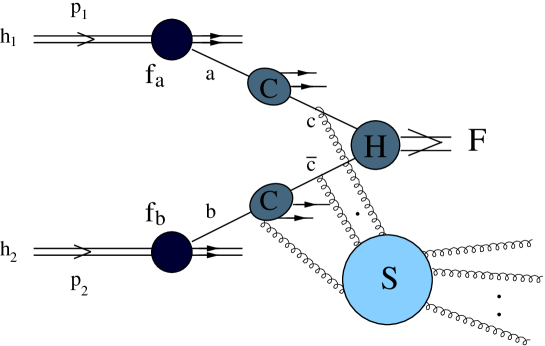
Figure 1: Diagrammatic structure of the various factors that enter the process-independent resummation formula (13).

The two versions (4) and (13) of the resummation formula can formally be related as follows. We use the renormalization-group identity

$$g_{1}(\alpha_{\mathrm{S}}(Q^{2}))=\exp\left\{\int_{b_{0}^{2}/b^{2}}^{Q^{2}}\frac{dq^{2}}{q^{2}}\;g_{2}(\alpha_{\mathrm{S}}(q^{2}))\right\}\;g_{1}(\alpha_{\mathrm{S}}(b_{0}^{2}/b^{2}))\;\;,$$ (16)

which is valid when

$$g_{2}(\alpha_{\mathrm{S}})=\beta(\alpha_{\mathrm{S}})\frac{d\ln g_{1}(\alpha_{\mathrm{S}})}{d\ln\alpha_{\mathrm{S}}}\;\;,$$ (17)

where $\beta(\alpha_{\mathrm{S}})$ is the QCD $\beta$-function

$$\frac{d\ln\alpha_{\mathrm{S}}(q^{2})}{d\ln q^{2}}=\beta(\alpha_{\mathrm{S}}(q^{2}))\;\;,$$ (18)

$$\beta(\alpha_{\mathrm{S}})=-\beta_{0}\frac{\alpha_{\mathrm{S}}}{\pi}-\beta_{1}\left(\frac{\alpha_{\mathrm{S}}}{\pi}\right)^{2}+\dots\;\;,\quad 12\beta_{0}=11C_{A}-2N_{f}\;\;.$$ (19)

Then, setting $g_{1}(\alpha_{\mathrm{S}}(Q^{2}))=H_{c}^{F}(\alpha_{\mathrm{S}}(Q^{2}))$ and inserting the right-hand side of Eq. (16) in Eq. (13), we immediately obtain Eq. (4). More precisely, the process-independent resummation formula in Eq. (13) implies the customary version in Eq. (4), provided the perturbative function $B_{c}(\alpha_{\mathrm{S}})$ in the form factor $S_{c}^{F}$ (see Eq. (5)) and the coefficient functions $C_{ab}^{F}$ are related to their process-independent analogues by the following all-order relations

$$C_{ab}^{F}(\alpha_{\mathrm{S}},z) = \left[H_{a}^{F}(\alpha_{\mathrm{S}})\right]^{1/2}\;C_{ab}(\alpha_{\mathrm{S}},z)\;\;,$$ (20)

$$B_{c}^{F}(\alpha_{\mathrm{S}}) = B_{c}(\alpha_{\mathrm{S}})-\beta(\alpha_{\mathrm{S}})\;\frac{d\ln H_{c}^{F}(\alpha_{\mathrm{S}})}{d\ln\alpha_{\mathrm{S}}}\;\;.$$ (21)

While the perturbative function $A_{c}(\alpha_{\mathrm{S}})$ and the first-order coefficient $B_{c}^{(1)}$ of the function $B_{c}(\alpha_{\mathrm{S}})$ are process-independent, the result in Eqs. (21) and (20) shows that the coefficients $B_{c}^{(2)},B_{c}^{(3)},\dots$ and $C_{ab}^{(1)}(z),C_{ab}^{(2)}(z),\dots$ in Eq. (4) do depend on the process. The process dependence of the first few coefficients is explicitly given by

$$C_{ab}^{(1)\,F}(z) = C_{ab}^{(1)}(z)+\delta_{ab}\;\delta(1-z)\;\frac{1}{2}\;H_{a}^{(1)\,F}\;\;,$$ (22)

$$C_{ab}^{(2)\,F}(z) = C_{ab}^{(2)}(z)+\frac{1}{2}\;H_{a}^{(1)\,F}\;C_{ab}^{(1)}(z)+\delta_{ab}\;\delta(1-z)\;\frac{1}{2}\;\left[H_{a}^{(2)\,F}-\frac{1}{4}\left(H_{a}^{(1)\,F}\right)^{2}\right]\;,$$ (23)

$$B_{c}^{(2)\,F} = B_{c}^{(2)}+\beta_{0}H_{c}^{(1)\,F}\;\;,$$ (24)

$$B_{c}^{(3)\,F} = B_{c}^{(3)}+\beta_{1}H_{c}^{(1)\,F}+2\beta_{0}\left[H_{c}^{(2)\,F}-\frac{1}{2}\left(H_{c}^{(1)\,F}\right)^{2}\right]\;\;.$$ (25)

Note that the process dependence of the resummation formula (4) is not simply embodied in pure numerical coefficients. For example, considering the Higgs production mechanism $g+g\rightarrow H$ through a massive-quark loop, the corresponding coefficient $H_{g}^{(1)\,H}$ and, hence, the form-factor coefficient $B_{g}^{(2)\,H}$ depend on the mass of the quark in the triangular loop. Moreover, the results discussed so far can straightforwardly be extended to more general configurations, in which several kinematical variables (and not only the invariant mass $Q$) of the final-state system $F$ are measured. For example, when $F$ is a pair of vector bosons, we can consider the corresponding transverse-momentum cross section at fixed rapidities of the vector bosons. The extension simply amounts to including the dependence on the kinematics of the system $F$ in the cross section factor $\sigma_{c{\bar{c}}}^{F}$ (and, hence, in $\sigma_{c{\bar{c}}}^{(LO)\,F}$ and $H_{c}^{F}$) of the process-independent resummation formula (13). In this general case, Eqs. (21) and (20) imply that the form factor $S_{c}^{F}$ and the coefficient functions $C_{ab}^{F}$ in Eq. (4) depend on the kinematics of the system $F$ in a non-trivial manner.

The process-independent resummation formula (13) can alternatively be used to relate the factors on the right-hand side of Eq. (4) for different processes. Considering Eqs. (21) and (20) for two different processes $F$ and $\widetilde{F}$, we obtain

$$C_{cb}^{F}(\alpha_{\mathrm{S}},z) = \left[H_{c}^{F{\widetilde{F}}}(\alpha_{\mathrm{S}})\right]^{1/2}\;C_{cb}^{\widetilde{F}}(\alpha_{\mathrm{S}},z)\;\;,$$ (26)

$$B_{c}^{F}(\alpha_{\mathrm{S}}) = B_{c}^{\widetilde{F}}(\alpha_{\mathrm{S}})-\beta(\alpha_{\mathrm{S}})\;\frac{d\ln H_{c}^{F{\widetilde{F}}}(\alpha_{\mathrm{S}})}{d\ln\alpha_{\mathrm{S}}}\;\;,$$ (27)

where $H^{F{\widetilde{F}}}=H^{F}/H^{\widetilde{F}}$. The perturbative expansion of these equations obviously leads to relations that are similar to those in Eqs. (22)–(24):

$$C_{cb}^{(1)\,F}(z) \!\!\!=\!\!\! C_{cb}^{(1)\,{\widetilde{F}}}(z)+\delta_{cb}\;\delta(1-z)\;\frac{1}{2}\,H_{c}^{(1)\,F{\widetilde{F}}}\;\;,$$ (28)

$$C_{cb}^{(2)\,F}(z) \!\!\!=\!\!\! C_{cb}^{(2)\,{\widetilde{F}}}(z)+\frac{1}{2}H_{c}^{(1)\,F{\widetilde{F}}}C_{cb}^{(1)\,{\widetilde{F}}}(z)+\delta_{cb}\,\delta(1-z)\frac{1}{2}\left[H_{c}^{(2)\,F{\widetilde{F}}}-\frac{1}{4}\left(H_{c}^{(1)\,F{\widetilde{F}}}\right)^{2}\right],$$ (29)

$$B_{c}^{(2)\,F} \!\!\!=\!\!\! B_{c}^{(2)\,{\widetilde{F}}}+\beta_{0}H_{c}^{(1)\,F{\widetilde{F}}}\;\;,$$ (30)

$$B_{c}^{(3)\,F} \!\!\!=\!\!\! B_{c}^{(3)\,{\widetilde{F}}}+\beta_{1}H_{c}^{(1)\,F{\widetilde{F}}}+2\beta_{0}\left[H_{c}^{(2)\,F{\widetilde{F}}}-\frac{1}{2}\left(H_{c}^{(1)\,F{\widetilde{F}}}\right)^{2}\right]\;\;.$$ (31)

Since the function $H^{F{\widetilde{F}}}$ does not appear in Eq. (4), within the framework of the process-dependent resummation formulae, Eqs. (26)–(31) have to be regarded as non-linear relations between the form factors and coefficient functions of different processes. For instance, having computed the first-order coefficient $C_{ab}^{(1)}$ for two processes, one can check Eq. (28) and extract $H_{c}^{(1)\,F{\widetilde{F}}}$. Then, the second-order coefficients $B_{c}^{(2)}$ of these processes must be related by Eq. (30). This constraint can either be checked or used to compute $B_{c}^{(2)\,{\widetilde{F}}}$ from $B_{c}^{(2)\,F}$.

The relation in Eq. (28) (or Eq. (22)) can straightforwardly be checked by comparing the known first-order coefficients $C_{ab}^{(1)\,F}(z)$ for the production of DY lepton pairs [12, 14, 15, 17], diphotons [18] and $ZZ$ pairs [19]. In particular, we have

$$H_{q}^{(1)\,F\,DY}=H_{q}^{(1)\,F}-H_{q}^{(1)\,DY}=\frac{1}{2}\;C_{F}\left({\cal V}^{F}-\pi^{2}+8\right)\;\;,\quad F=\gamma\gamma,ZZ\;\;,$$ (32)

where ${\cal V}^{\gamma\gamma}$ and ${\cal V}^{ZZ}$ are given in Eq. (11) of Ref. [18] and in Eq. (8) of Ref. [19], respectively. The relation (30) (or (24)) for the NNLL coefficient $B^{(2)\,F}$ has explicitly been derived by the process-independent calculation at ${\cal O}(\alpha_{\mathrm{S}}^{2})$ performed in Ref. [13].

The reasoning used to obtain Eq. (4) from Eq. (13) can also be used to show that Eq. (13) is invariant under the transformation

$$H_{c}^{F}(\alpha_{\mathrm{S}}(Q^{2})) \rightarrow H_{c}^{F}(\alpha_{\mathrm{S}}(Q^{2}))\;\left[g(\alpha_{\mathrm{S}}(Q^{2}))\right]^{-1}\;,$$

$$S_{c}(Q,b) \rightarrow S_{c}(Q,b)\;\exp\left\{\int_{b_{0}^{2}/b^{2}}^{Q^{2}}\frac{dq^{2}}{q^{2}}\;\beta(\alpha_{\mathrm{S}}(q^{2}))\;\frac{d\ln g(\alpha_{\mathrm{S}}(q^{2}))}{d\ln\alpha_{\mathrm{S}}(q^{2})}\right\}\;,$$ (33)

$$C_{ab}(\alpha_{\mathrm{S}}(b_{0}^{2}/b^{2}),z) \rightarrow C_{ab}(\alpha_{\mathrm{S}}(b_{0}^{2}/b^{2}),z)\;\left[g(\alpha_{\mathrm{S}}(b_{0}^{2}/b^{2}))\right]^{1/2}\;,$$

where $g(\alpha_{\mathrm{S}})=1+{\cal O}(\alpha_{\mathrm{S}})$ is an arbitrary perturbative function. This renormalization-group symmetry of the resummation formula (13) implies that its factors, $H_{c}^{F},S_{c}$ (more precisely, the function $B_{c}$) and $C_{ab}$, although they are process-independent, are not unambiguously computable (defined) order by order in perturbation theory. The same conclusion can be reached by expanding Eq. (13) in powers of $\alpha_{\mathrm{S}}$. At any given order in $\alpha_{\mathrm{S}}$, the coefficients of the various powers of $\ln Q^{2}b^{2}$ depend on the unknowns $H_{c}^{(n)\,F},C_{ab}^{(n)},B_{c}^{(n)}$, but the number of such coefficients is less that the number of unknowns. For instance, at the first relative order in $\alpha_{\mathrm{S}}$, the coefficient of $\ln^{2}Q^{2}b^{2}$ determines $A^{(1)}$, the coefficient of $\ln Q^{2}b^{2}$ determines $B^{(1)}$, while the coefficient of the constant term is a linear combination of $H^{(1)\,F}$ and $C_{ab}^{(1)}$.

The perturbative ambiguity of the decomposition of the right-hand side of Eq. (13) in the factors $H_{c}^{F},S_{c}$ and $C_{ab}$ is a consequence of the fact that the transverse-momentum cross section is not a collinear-safe quantity. The effect of collinear radiation at low transverse-momentum scales, $q_{t}\raisebox{-1.72218pt}{\hbox to0.0pt{$\,\sim\,$\hss}}\raisebox{1.72218pt}{$\,<\,$}1/b$, is divergent in perturbation theory. The (arbitrary) regularization procedure of these divergences introduces some ambiguity in the definition of the coefficient functions $C_{ab}$. Then, the ambiguity propagates to $S_{c}$ and $H_{c}^{F}$ through collinear evolution (see Eq. (16)). In this way of thinking, the ambiguity is similar to that encountered in the definition of the parton densities. As the parton densities have to be defined by fixing a factorization scheme (e.g. the ${\overline{\rm MS}}$ scheme or the DIS scheme), the factors on the right-hand side of Eq. (13) has to be defined by choosing a ‘resummation scheme’. Note that the choice of a ‘resummation scheme’ amounts to defining $H_{c}^{F}$ (or $C_{ab}$) for a single process. Having done that, the process-dependent factor $H_{c}^{F}$ and the universal factors $S_{c}$ and $C_{ab}$ in Eq. (13) are unambiguously determined for any other process in Eq. (1).

We can suggest three examples of ‘resummation schemes’, that is three prescriptions to use the process-independent factorization formula (13) in practice. A first ‘short-cut’ (because the DY transverse-momentum distribution is best studied) prescription, which we name ‘DY resummation scheme’, is obtained by setting $H_{q}^{DY}(\alpha_{\mathrm{S}})\equiv 1$ in the case of the DY cross section (integrated over the rapidity of the vector boson). This unambiguously fixes the process-independent form factor $S_{c}$ and coefficients functions $C_{ab}$ as those determined from the DY process. In particular, the coefficient $B_{q}^{(2)}$ of the quark form factor is that in Eq. (11), and the quark coefficient functions $C_{qb}^{(1)}(z)$ $(b=q,{\bar{q}},g)$ are those computed in Refs. [12, 14, 15, 17] for the DY process. Any other $q{\bar{q}}$-initiated cross section is then obtained by using Eq. (13) with a perturbatively computable hard function $H_{q}^{F}(\alpha_{\mathrm{S}})$. This prescription can be extended to $gg$-initiated cross sections by setting $H_{g}^{H}(\alpha_{\mathrm{S}})\equiv 1$ in the case of Higgs production via $gg$ fusion. Thus, in the case of an infinitely-massive quark in the loop (the definition of the scheme will be different by keeping the mass of the quark finite), the coefficient $B_{g}^{(2)}$ of the gluon form factor is that given in Eq. (12) and the gluon coefficient functions $C_{gb}^{(1)}(z)$ $(b=q,{\bar{q}},g)$ are those computed in Ref. [16].

A second prescription, which is in some sense more physical, exploits the fact that the first moment (with respect to $Q^{2}/s$) of the flavour non-singlet (NS) hadronic (and partonic) cross sections defines collinear-safe quantities. This property follows from fermion-number conservation. Thus, we can define a ‘NS resummation scheme’ by fixing the overall normalization of the NS coefficient function $C_{ab}(\alpha_{\mathrm{S}},z)$ in Eq. (13) in such a way that its first moment (with respect to $z$) vanishes. In this scheme (the subscript NS labels the scheme choice)

$$\int_{0}^{1}dz\;\left[\;C_{qq,NS}(\alpha_{\mathrm{S}},z)-C_{q{\bar{q}},NS}(\alpha_{\mathrm{S}},z)\;\right]\equiv 1\;\;,$$ (34)

and thus, using the DY coefficients functions from Refs. [12, 14, 15, 17] and Eq. (22), we obtain

$$H^{(1)\,DY}_{q,NS}=C_{F}\left(\frac{\pi^{2}}{2}-\frac{7}{2}\right)\;\;.$$ (35)

Inserting Eq. (35) in Eq. (24), and using the DY coefficient in Eq. (11), we then obtain the corresponding coefficient of the quark form factor:

$$\!\!B_{q,NS}^{(2)} \!\!\!\!=\!\!\!\! B_{q}^{(2)\,DY}-\beta_{0}H^{(1)\,DY}_{q,NS}$$ (36)

$$\!\!\!\!=\!\!\!\! C_{F}^{2}\left(\frac{\pi^{2}}{4}-\frac{3}{16}-3\zeta_{3}\right)+C_{F}\,C_{A}\left(-\frac{11}{72}\pi^{2}-\frac{13}{16}+\frac{3}{2}\zeta_{3}\right)+C_{F}\,N_{f}\left(\frac{1}{8}+\frac{\pi^{2}}{36}\right).$$

The reason why this scheme can be considered ‘more physical’ is that the first moments of the NS cross sections are collinear-safe and, hence, free from ambiguities related to the regularization procedure of collinear singularities. As is known [9, 11, 20], the process-independent form factor coefficients in Eq. (9) measure the physical intensity of soft ($A_{c}^{(1)}$ and $A_{c}^{(2)}$) and collinear $(B_{c}^{(1)})$ radiation. Since the coefficient $B_{q,NS}^{(2)}$ in Eq. (36) appears in the form factor of an infrared and collinear safe quantity, it should measure the intensity of the collinear radiation from quarks at the second order in $\alpha_{\mathrm{S}}$ and it should enter in the form factor of other infrared and collinear safe quantities. For example, an analogous transverse-momentum form factor controls the back-to-back region of the energy–energy correlation (EEC) in $e^{+}e^{-}$ annihilation [21]. The coefficient in Eq. (36) should directly be related to the corresponding coefficient $B^{(2)}$ of the EEC, modulo (possible) effects due to the difference between the space-like kinematics of the transverse-momentum cross sections and the time-like kinematics of $e^{+}e^{-}$ annihilation.

The generalization of the ‘NS resummation scheme’ to $gg$-fusion processes can be obtained, for instance, by fixing the overall normalization of the gluon coefficient function $C_{gg}(\alpha_{\mathrm{S}},z)$ in Eq. (13) in such a way that its first moment vanishes. Note, however, that in the gluon (or, more generally, flavour-singlet) channel there is no anologue of the fermion-number conservation rule. Flavour-singlet transverse-momentum cross sections are collinear unsafe quantities. Thus, a ‘physical’ (collinear-safe) interpretation of the higher-order coefficients of the function $B_{g}(\alpha_{\mathrm{S}})$ of the gluon form factor is less straightforward than in the quark channel.

The coefficient $B_{c}^{(1)}$ in Eq. (9) coincides with the coefficient of the end-point contribution (the term proportional to $\delta(1-z)$) to the LO Altarelli–Parisi probability $P_{cc}^{(1)}(z)$. As can be noticed from Eqs. (22) and (23) in Ref. [13], the coefficient $B_{q,NS}^{(2)}$ in Eq. (36) (and the coefficients $B_{q}^{(2)\,DY}$ and $B_{g}^{(2)\,H}$ in Eqs. (11) and (12)) does not coincide with that of the end-point contribution to the NLO Altarelli–Parisi probability $P_{cc}^{(2)\,{\overline{\rm MS}}}(z)$ in the ${\overline{\rm MS}}$ factorization scheme. This should not be surprising, because beyond LO the Altarelli–Parisi probabilities are not collinear-safe quantities: they depend on the regularization procedure of the collinear singularities and on the factorization scheme. This interpretation is confirmed by the fact that the various coefficients $B_{c}^{(2)}$ differ from one another by terms proportional to the first coefficient $\beta_{0}$ of the $\beta$-function, as should be expected from factorization-scheme dependence. Using Eqs. (20)–(25), it is obviously possible to introduce an ‘${\overline{\rm MS}}$ resummation scheme’ such that the function $B_{c}(\alpha_{\mathrm{S}})$ of the process-independent form factor in Eqs. (5) and (13) coincides by definition with the perturbative function $B_{c,{\overline{\rm MS}}}(\alpha_{\mathrm{S}})$ that controls the end-point contribution to the all-order Altarelli–Parisi probabilities in the ${\overline{\rm MS}}$ factorization scheme.

Note that our discussion on the relation between Eqs. (4) and (13) and on the resummation-scheme ambiguity does not imply that the two equations are equivalent. In fact, the process-independent resummation framework contains more information than its customary process-dependent version. To evaluate resummed cross section within the framework of Eq. (4), we should compute two functions ($S_{c}^{F}$ and $C_{ab}^{F}$) for each process $F$. Once a ‘resummation scheme’ has been defined, a similar evaluation by using Eq. (13) requires the computation of two universal functions ($S_{c}$ and $C_{ab}$) and of a single additional function $(H_{c}^{F})$ for each process.

Of course, we can still continue to use Eq. (4). In this case, we can exploit the additional information contained in Eq. (13) by using Eqs. (26) and (27) (or their perturbative expansions in Eqs. (28)–(31)) to relate form factors and coefficient functions for different processes.

Independently of the resummation formula that is actually used, once the form factor coefficient $B_{c}^{(2)}$ has been computed for a single process by performing a calculation at relative order $\alpha_{\mathrm{S}}^{2}$, no further ${\cal O}(\alpha_{\mathrm{S}}^{2})$-calculation is necessary for its universal implementation in all processes. The implementation can simply be performed by computing the coefficient functions at ${\cal O}(\alpha_{\mathrm{S}})$ and then using Eqs. (22) and (24) (or Eqs. (28) and (30)). Analogously, using Eqs. (23) and (25) (or Eqs. (29) and (31)), the universal implementation of the form factor coefficient $B_{c}^{(3)}$ requires its ${\cal O}(\alpha_{\mathrm{S}}^{3})$ computation in a single process and the evaluation of the coefficient functions at ${\cal O}(\alpha_{\mathrm{S}}^{2})$ for the various processes. This procedure extends to any higher orders.

At present, owing to the results in Eqs. (11) and (12), the NNLL coefficient $B_{c}^{(2)}$ can be included in all calculations of transverse-momentum cross sections in hadron collisions. Its inclusion cannot be regarded as the extension of these resummed calculations to full NNLL accuracy, because the corresponding coefficient $A_{c}^{(3)}$ is not yet known. Nonetheless, the knowledge of $B_{c}^{(2)}$ can certainly be used to improve the matching with fixed-order calculations at high $q_{\perp}$. The matching can be performed by supplementing the resummed cross section with the finite contribution on the right-hand side of Eq. (2). The finite contribution is obtained, from the complete calculation at a fixed order in $\alpha_{\mathrm{S}}$, by subtraction of the corresponding perturbative terms already included in the resummed component. If $B_{c}^{(2)}$ is included in this component, the remaining finite component at relative order $\alpha_{\mathrm{S}}^{2}$ contains no $\ln Q^{2}/q_{\perp}^{2}$ terms. Thus, the latter can be inserted in Eq. (2) uniformly with respect to $q_{\perp}$, that is without including logarithmic terms that spoil the convergence of the matched result in the small-$q_{\perp}$ region.

In this paper we have not discussed how non-perturbative effects (see Refs. [22]–[27] and references therein) affect the transverse-momentum cross sections. Although the process-independent resummation formula (13) can be recast in the form of Eq. (4) at the perturbative level, it is not evident whether the two formulations are equally suitable to deal with non-perturbative contributions. In particular, since the form factor $S_{c}^{F}$ and the coefficient functions $C_{ab}^{F}$ in Eq. (4) are process-dependent, a simple and uniform implementation of process-independent non-perturbative effects (such as those due to the initial intrinsic $k_{t}$ of the partons in the colliding hadrons) in Eq. (4) can be very involved. The process-independent version (13) of the resummed cross section can help to consistently introduce and implement non-perturbative effects in transverse-momentum distributions.

We conclude by discussing the dependence of the resummation formulae on the renormalization and factorization scales $\mu_{R}$ and $\mu_{F}$. This dependence is often parametrized by introducing some arbitrary coefficients, $C_{1},C_{2},C_{3},$ as suggested in Refs. [8, 10]. This is a perfectly sensible and reasonable procedure to try to estimate the effect of higher-order corrections, but it does not exactly correspond to the procedure that is usually followed in fixed-order perturbative calculations. In the case of soft-gluon resummed calculations for event shapes and jet rates in $e^{+}e^{-}$ annihilation and for threshold contributions in hadronic cross sections, a different procedure was introduced in Refs. [28] and [29]. The latter procedure closely matches the use of $\mu_{R}$ and $\mu_{F}$ in fixed-order calculations, and it can directly be applied (see, e.g., Refs. [28, 29] and several other references quoted in Section 5 of Ref. [1]) to compare the scale dependence of resummed and fixed-order predictions. Here, we would like to note that the procedure of Refs. [28, 29] can be introduced also in the case of the transverse-momentum distributions.

To this purpose, we first perform the replacement $f_{a/h}(x,b_{0}^{2}/b^{2})\rightarrow f_{a/h}(x,\mu_{F}^{2})$ in Eq. (3) and we rewrite the resummed component of the transverse-momentum cross section as

$$\left[\frac{d\sigma_{F}}{dQ^{2}\;dq_{\perp}^{2}}\right]_{{\rm res.}} = \sum_{a,b}\int_{0}^{1}dx_{1}\int_{0}^{1}dx_{2}\;f_{a/h_{1}}(x_{1},\mu_{F}^{2})\;f_{b/h_{2}}(x_{2},\mu_{F}^{2})$$ (37)

$$\cdot \int_{0}^{\infty}db\;\frac{b}{2}\;J_{0}(bq_{\perp})\;W_{ab}^{F}(x_{1}x_{2}s;Q,b,\mu_{F})\;\;.$$

To obtain Eq. (37) we have simply used the scale dependence of the parton densities as given by

$$f_{a/h}(x,b_{0}^{2}/b^{2})=\sum_{b}\int_{x}^{1}\frac{dz}{z}\;U_{ab}(z;b_{0}^{2}/b^{2},\mu_{F}^{2})\;f_{b/h}(x/z,\mu_{F}^{2})\;\;,$$ (38)

where $U_{ab}(z;b_{0}^{2}/b^{2},\mu_{F}^{2})$ is the customary evolution operator matrix obtained by solving the Altarelli-Parisi evolution equations to the required logarithmic accuracy. The resummed partonic cross section in Eq. (37) is thus obtained from that in Eq. (13) (or (4)) by replacing the coefficient functions $C_{ca}(\alpha_{\mathrm{S}}(b_{0}^{2}/b^{2}),x)$ (or $C_{ca}^{F}(\alpha_{\mathrm{S}}(b_{0}^{2}/b^{2}),x)$) with the following convolution

$$C_{ca}(\alpha_{\mathrm{S}}(b_{0}^{2}/b^{2}),x;\mu_{F}^{2})=\sum_{b}\int_{x}^{1}\frac{dz}{z}\;C_{cb}(\alpha_{\mathrm{S}}(b_{0}^{2}/b^{2}),z)\;U_{ba}(z;b_{0}^{2}/b^{2},\mu_{F}^{2})\;\;.$$ (39)

Note that, unlike the parton densities in Eq. (3), those in Eq. (37) do not depend on the impact parameter $b$, but only on the factorization scale $\mu_{F}$. Expression (37) can thus be useful in practical calculations, because it avoids the numerical integration of the parton densities with respect to the impact parameter. The only factor of the resummed cross section that has to be integrated over $b$ is now the perturbative component $W_{ab}^{F}(x_{1}x_{2}s;Q,b,\mu_{F})$.

Then, to proceed as in Refs. [28, 29], we simply observe that we can choose $\mu_{F}$ and $\mu_{R}$ to be of the order of the hard scale $Q$. Thus, $W_{ab}^{F}(x_{1}x_{2}s;Q,b,\mu_{F})$ contains only an additional large parameter, $L\equiv\ln Q^{2}b^{2}$, and it can be written as

$$W^{F}(Q,b,\mu_{F}) \sim \exp\left\{L\;f_{1}\left(\alpha_{\mathrm{S}}L\frac{}{}\right)+f_{2}\left(\alpha_{\mathrm{S}}L;\frac{Q}{\mu_{R}},\frac{Q}{\mu_{F}}\right)+\alpha_{\mathrm{S}}f_{3}\left(\alpha_{\mathrm{S}}L;\frac{Q}{\mu_{R}},\frac{Q}{\mu_{F}}\right)+\dots\right\}$$ (40)

$$\cdot \sigma^{F}(Q^{2},\alpha_{\mathrm{S}};Q^{2}/\mu_{R}^{2})\;\;,$$

where $\alpha_{\mathrm{S}}=\alpha_{\mathrm{S}}(\mu_{R}^{2})$. The notation on the right-hand side is symbolical, because we have understood the dependence on the momentum fractions  $z_{1},z_{2}$ and on the parton indices $a,b=q,{\bar{q}},g$. In particular, the exponential should be understood as an exponential matrix that depends on the parton indices.

The form in Eq. (40) is straightforwardly obtained by using the exponentiated result in Eq. (5) for the form factor and the customary exponential form for the evolution operator $U_{ab}(z;b_{0}^{2}/b^{2},\mu_{F}^{2})$. In the exponent, the function $Lf_{1}$ resums all the LL contributions $\alpha_{\mathrm{S}}^{n}L^{n+1}$, the function $f_{2}$ resums the NLL terms $\alpha_{\mathrm{S}}^{n}L^{n}$, while $\alpha_{\mathrm{S}}f_{3}$ contains the NNLL terms $\alpha_{\mathrm{S}}^{n}L^{n-1}$, and so forth. The functions $f_{i}$ are normalized as $f_{i}(\alpha_{\mathrm{S}}L=0)=0$ and can easily be obtained in analytic form.

Although it is symbolical, the form of Eq. (40) is sufficient to make our point. Indeed, it is exactly in the same form as the expressions that are obtained by performing soft-gluon resummation for $e^{+}e^{-}$ event shapes and hadronic cross sections near threshold. Recasting the resummed transverse-momentum distributions in the form of Eq. (40), the theoretical accuracy of the resummed calculation can be investigated as in fixed-order calculations, by varying $\mu_{F}$ and $\mu_{R}$ around the value $Q$ of the typical hard scale. Future studies along these lines (for instance, comparisons of the scale dependence of resummed and fixed-order calculations) could be useful to increase our confidence in the quantitative reliability of resummed predictions for transverse-momentum cross sections.

References

- [1] S. Catani et al., hep-ph/0005025, in the Proceedings of the CERN Workshop on Standard Model Physics (and more) at the LHC, Eds. G. Altarelli and M.L. Mangano (CERN 2000-04, Geneva, 2000), p. 1.
- [2] S. Catani et al., hep-ph/0005114, to be published in the Proceedings of the Les Houches Workshop on Physics at TeV Colliders, Eds. P. Aurenche et al.
- [3] U. Baur et al., hep-ph/0005226, to appear in the Proceedings of the Fermilab Workshop on QCD and Weak Boson Physics at Run II.
- [4] Y. L. Dokshitzer, D. Diakonov and S. I. Troian, Phys. Rep. 58 (1980) 269.
- [5] G. Parisi and R. Petronzio, Nucl. Phys. B154 (1979) 427.
- [6] G. Curci, M. Greco and Y. Srivastava, Nucl. Phys. B159 (1979) 451.
- [7] A. Bassetto, M. Ciafaloni and G. Marchesini, Nucl. Phys. B163 (1980) 477.
- [8] J. C. Collins and D. E. Soper, Nucl. Phys. B193 (1981) 381 (E ibid. B213 (1983) 545), Nucl. Phys. B197 (1982) 446.
- [9] J. Kodaira and L. Trentadue, Phys. Lett. B112 (1982) 66, Phys. Lett. B123 (1983) 335.
- [10] J. C. Collins, D. E. Soper and G. Sterman, Nucl. Phys. B250 (1985) 199.
- [11] S. Catani, E. D’Emilio and L. Trentadue, Phys. Lett. B211 (1988) 335.
- [12] C. T. Davies and W. J. Stirling, Nucl. Phys. B244 (1984) 337.
- [13] D. de Florian and M. Grazzini, hep-ph/0008152.
- [14] G. Altarelli, R. K. Ellis, M. Greco and G. Martinelli, Nucl. Phys. B246 (1984) 12.
- [15] C. T. Davies, B. R. Webber and W. J. Stirling, Nucl. Phys. B256 (1985) 413.
- [16] R. P. Kauffman, Phys. Rev. D45 (1992) 1512.
- [17] C. Balazs and C. P. Yuan, Phys. Rev. D56 (1997) 5558.
- [18] C. Balazs, E. L. Berger, S. Mrenna and C. P. Yuan, Phys. Rev. D57 (1998) 6934.
- [19] C. Balazs and C. P. Yuan, Phys. Rev. D59 (1999) 114007.
- [20] S. Catani, B. R. Webber and G. Marchesini, Nucl. Phys. B349 (1991) 635.
- [21] See, e.g., Y. L. Dokshitzer, G. Marchesini and B. R. Webber, JHEP 9907 (1999) 012, and references therein.
- [22] R. K. Ellis, D. A. Ross and S. Veseli, Nucl. Phys. B503 (1997) 309.
- [23] F. Landry, R. Brock, G. Ladinsky and C. P. Yuan, preprint MSUHEP-90414 [hep-ph/9905391].
- [24] A. Guffanti and G. E. Smye, preprint CAVENDISH-HEP-00-04 [hep-ph/0007190].
- [25] R. K. Ellis and S. Veseli, Nucl. Phys. B511 (1998) 649.
- [26] S. Frixione, P. Nason and G. Ridolfi, Nucl. Phys. B542 (1999) 311.
- [27] A. Kulesza and W. J. Stirling, Nucl. Phys. B555 (1999) 279.
- [28] S. Catani, G. Turnock, B. R. Webber and L. Trentadue, Phys. Lett. B263 (1991) 491; S. Catani, L. Trentadue, G. Turnock and B. R. Webber, Nucl. Phys. B407 (1993) 3.
- [29] R. Bonciani, S. Catani, M. L. Mangano and P. Nason, Nucl. Phys. B529 (1998) 424; S. Catani, M. L. Mangano, P. Nason, C. Oleari and W. Vogelsang, JHEP 9903 (1999) 025.