A superformula for neutrinoless double beta decay II: The short range part

Abstract

A general Lorentz–invariant parameterization for the short-range part of the $0\nu\beta\beta$ decay rate is derived. Combined with the long range part already published this general parameterization in terms of effective $B-L$ violating couplings allows one to extract the $0\nu\beta\beta$ limits on arbitrary lepton number violating theories.

, , ,

1 Introduction

The search for neutrinoless double beta decay has been proven to be one of the most powerful tools to constrain $B-L$ violating physics beyond the standard model [1]. In recent years, besides the most restrictive limit on the effective neutrino Majorana mass [1, 2, 3], stringent constraints on several theories beyond the Standard Model such as $R$–parity violating [4, 5, 6] as well as conserving [7] SUSY, leptoquarks [8] and left–right symmetric models [9] have been derived (for a review see [1]). While the neutrino mass limit is based on the well-known mechanism exchanging a massive Majorana neutrino between two standard model $V-A$ vertices, the effective vertices appearing in the new contributions involve non–standard currents such as scalar, pseudoscalar and tensor currents. Moreover, besides contributions with a light neutrino being exchanged between two separated vertices, the so-called long-range part, additional contributions from the short range part are expected, e.g. in SUSY without R-parity [10, 11].

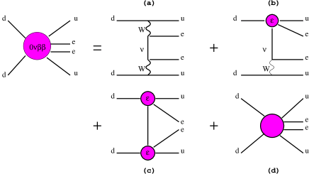
Figure 1: Feynman graphs of the general double beta rate: The contributions a) - c) correspond to the long range part discussed in [12], the contribution d) is the short range part.

Thus we felt motivated to consider the neutrinoless double beta decay rate in a general framework, parameterizing the new physics contributions in terms of all effective low-energy currents allowed by Lorentz-invariance (see Fig. 1). Such an ansatz allows one to separate the nuclear physics part of double beta decay from the underlying particle physics model, and to derive limits on arbitrary lepton number violating theories. The first step of this work, treating the long–range part (contributions a-c in Fig. 1), has been published in [12]. In the following the remaining part, treating the short range part (contribution d), is presented.

Although the general decay rate is independent of the underlying nuclear physics model, to extract quantitative limits, values of nuclear matrix elements are needed, which have been calculated in [11] in the (pn)QRPA aproach. Using these, for the first time limits for all potential new physics contributions are derived here.

2 General Parametrization

In the short range part the effective interaction can be considered as point-like, thus the decay rate results from first order perturbation theory,

$$R_{0\nu\beta\beta} = i\int d^{4}x\langle(Z+2,A),2e^{-}|{\cal L}(x)|(Z,A),-\rangle.$$ (1)

The most general Lorentz invariant Lagrangian has the following form

$${\cal L}=\frac{G^{2}_{F}}{2}m_{p}^{-1}\{\epsilon_{1}JJj+\epsilon_{2}J^{\mu\nu}J_{\mu\nu}j+\epsilon_{3}J^{\mu}J_{\mu}j+\epsilon_{4}J^{\mu}J_{\mu\nu}j^{\nu}+\epsilon_{5}J^{\mu}Jj_{\mu}$$

$$+\epsilon_{6}J^{\mu}J^{\nu}j_{\mu\nu}+\epsilon_{7}JJ^{\mu\nu}j_{\mu\nu}+\epsilon_{8}J_{\mu\alpha}J^{\nu\alpha}j^{\mu}_{\nu}\},$$ (2)

with the proton mass $m_{p}$ and the hadronic currents of defined chirality $J=\overline{u}(1\pm\gamma_{5})d$, $J^{\mu}=\overline{u}\gamma^{\mu}(1\pm\gamma_{5})d$, $J^{\mu\nu}=\overline{u}\frac{i}{2}[\gamma^{\mu},\gamma^{\nu}](1\pm\gamma_{5})d$ and the leptonic curents $j=\overline{e}(1\pm\gamma_{5})e^{C}$, $j^{\mu}=\overline{e}\gamma^{\mu}(1\pm\gamma_{5})e^{C}$ , $j^{\mu\nu}=\overline{e}\frac{i}{2}[\gamma^{\mu},\gamma^{\nu}](1\pm\gamma_{5})e^{C}$. In some of the cases the decay rate for the effective coupling $\epsilon_{\alpha}$ may depend also on the chirality of the currents involved. In these cases we define $\epsilon_{\alpha}=\epsilon^{xyz}_{\alpha}$, where $xyz=L/R,L/R,L/R$ defines the chirality of the hadronic and leptonic currents in the order of appearance in eq. (2). In the cases where it is not necessary to distinguish the different chiralities we suppress this additional index.

In renormalizable theories no fundamental tensors exist. Thus the tensor currents have to result either from Fierz rearrangements or by integrating out heavy particles, when deriving the effective Lagrangian from the fundamental theory and decomposing the expressions obtained in terms of the Lorentz invariant bilinears used above, e.g. from $\bar{u}\gamma_{\mu}\gamma_{\nu}(1+\gamma_{5})d=g_{\mu\nu}J-iJ_{\mu\nu}$. Moreover, the contribution of the leptonic tensor current vanishes in s-wave approximation. Since the tensor currents in the rearrangements and decompositions mentioned above are always created together with dominant contributions, the corresponding terms proportional to $\epsilon_{6},\epsilon_{7},\epsilon_{8}$ can be neglected. The remaining terms are the ones proportional to $\epsilon_{1},\epsilon_{2},\epsilon_{3},\epsilon_{4},\epsilon_{5}$.

Applying the standard nuclear theory methods based on the non-relativistic impulse approximation we derive the general $0\nu\beta\beta$-decay half-life formula in s–wave approximation

$$[T_{1/2}^{0\nu\beta\beta}]^{-1}=$$ (3)

$$G_{1}|\sum_{i=1}^{3}\epsilon_{i}{\cal M}_{i}|^{2}+G_{2}|\sum_{i=4}^{5}\epsilon_{i}{\cal M}_{i}|^{2}+G_{3}{\rm Re}[(\sum_{i=1}^{3}\epsilon_{i}{\cal M}_{i})(\sum_{i=4}^{5}\epsilon_{i}{\cal M}_{i})^{*}].$$

Here the phase space factors are

$$G_{1}=G_{01},\ \ \ G_{2}=\frac{(m_{e}R)^{2}}{8}G_{09},\ \ \ G_{3}=\left(\frac{m_{e}R}{4}\right)G_{06},$$ (4)

with $G_{0k}$ given in [13] and shown in Table 1.

The nuclear matrix elements in eq. (3) are

$${\cal M}_{1}=-\alpha_{1}{\cal M}_{F,N},\ \ \ {\cal M}_{2}=-\alpha_{2}{\cal M}_{GT,N},$$

$${\cal M}_{3}=\frac{m_{A}^{2}}{m_{P}m_{e}}\{{\cal M}_{GT,N}\mp\alpha_{3}{\cal M}_{F,N}\},$$ (5)

$${\cal M}_{4}=\pm\alpha_{4}{\cal M}_{GT,N},\ \ \ {\cal M}_{5}=\mp\alpha_{5}{\cal M}_{F,N}.$$

In the last three cases contractions of hadronic currents with different chiralities lead to different results. The negative sign in ${\cal M}_{3}$ corresponds to $\epsilon_{3}^{LLz}$ and $\epsilon_{3}^{RRz}$ ($J_{V\mp A}J_{V\mp A}$), the positive sign to $\epsilon_{3}^{LRz}$ and $\epsilon_{3}^{RLz}$ ($J_{V\mp A}\-J_{V\pm A}$). The sign of ${\cal M}_{4}$ is positive for the combinations $\epsilon_{4}^{LLL}$, $\epsilon_{4}^{RRL}$, $\epsilon_{4}^{RLR}$, $\epsilon_{4}^{LRR}$ ($J_{V\mp A}J_{TL/TR}j_{V-A}$ and $J_{V\pm A}J_{TL/TR}j_{V+A}$). For the combinations $\epsilon_{4}^{LLR}$, $\epsilon_{4}^{RRR}$, $\epsilon_{4}^{RLL}$, $\epsilon_{4}^{LRL}$ ($J_{V\mp A}J_{TL/TR}j_{V+A}$ and $J_{V\pm A}J_{TL/TR}j_{V-A}$) it is negative. The sign of the matrix element ${\cal M}_{5}$ is negative for the left-handed leptonic current ($\epsilon_{5}^{xyL}$) and positive for the right-handed one ($\epsilon_{5}^{xyR}$).

The standard nuclear matrix elements ${\cal M}_{F,N}$ und ${\cal M}_{GT,N}$ in eq. (2) are defined as

$${\cal M}_{GT,N}=\big{<}F|\sum_{i\neq j}\tau_{+}^{(i)}\tau_{+}^{(j)}\vec{\sigma}_{i}\cdot\vec{\sigma}_{j}\left(\frac{R_{0}}{r_{ij}}\right)F_{N}(x_{A})|I\big{>},$$ (6)

$${\cal M}_{F,N}=\big{<}F|\sum_{i\neq j}\tau_{+}^{(i)}\tau_{+}^{(j)}\left(\frac{R_{0}}{r_{ij}}\right)F_{N}(x_{A})|I\big{>}.$$ (7)

Here $r_{ij}$ and $R_{0}$ are the distance of the nucleons involved and the nuclear radius respectively. Numerical values of these matrix elements for ⁷⁶Ge [11] in the Quasi Particle Random Phase Approximation(pn-QRPA) are given in Table 1. Uncertainties of nuclear matrix element calculations are discussed in Ref. [11, 14].

The prefactors $\alpha_{i}$ in eq. (2) are defined as follows,

$$\alpha_{1}=\Big{(}\frac{F_{S}^{(3)}}{g_{A}}\Big{)}^{2}\cdot\frac{m_{A}^{2}}{m_{P}m_{e}},\ \ \ \alpha_{2}=8\Big{(}\frac{T_{1}^{(3)}}{g_{A}}\Big{)}^{2}\cdot\frac{m_{A}^{2}}{m_{P}m_{e}},$$ (8)

$$\alpha_{3}=\Big{(}\frac{g_{V}}{g_{A}}\Big{)}^{2},\ \ \ \alpha_{4}=\frac{T_{1}^{(3)}}{g_{A}}\cdot\frac{m_{A}^{2}}{m_{P}m_{e}}\ \ \ \alpha_{5}=\frac{g_{V}F_{S}^{(3)}}{g_{A}^{2}}\cdot\frac{m_{A}^{2}}{m_{P}m_{e}}.$$

The finite nucleon size is taken into account in a common way [15] by introducing the nucleon form factors in a dipole form

$$\frac{g_{V,A}(q^{2})}{g_{V,A}}=\frac{F_{S}(q^{2})}{F_{S}}=\frac{T_{1}^{(3)}(q^{2})}{T_{1}^{(3)}}=\left(1-\frac{q^{2}}{m_{A}^{2}}\right)^{-2},$$ (9)

with $m_{A}=0.85$ GeV, $g_{V}=1.0,g_{A}=1.26$. The other form factor normalizations have been calculated in Ref. [16] within the MIT bag model,

$$F_{S}^{(3)}=0.48,\ \ \ T_{1}^{(3)}=1.38.$$ (10)

The momentum dependence has been absorbed into the integral over the momentum $q$ transferred between two nucleons,

$$F_{N}(x_{A})=4\pi m_{A}^{6}{r}_{ij}\int\frac{d^{3}\vec{q}}{(2\pi)^{3}}\frac{1}{(m_{A}^{2}+\vec{q}^{2})^{4}}e^{i\vec{q}\vec{r}_{ij}}=\frac{x_{A}}{48}(3+3x_{A}+x_{A}^{2})e^{-x_{A}},$$ (11)

where $x_{A}=m_{A}r_{ij}$.

3 General $0\nu\beta\beta$-decay constraints

Let us extract limits on the lepton-number violating parameters $\epsilon_{k}$ in eq. (3) from the experimental lower bound on the $0\nu\beta\beta$-decay half-life. The conservative half-life limit of the Heidelberg–Moscow experiment [2]

$$T_{1/2}^{0\nu\beta\beta}>1.8\cdot 10^{25}years(90\%C.L.)$$ (12)

provides at present the most stringent bound. Applying this limit to eq. (3) leads to a complex 5-dimensional exclusion plot for all five parameters $\epsilon_{k}$. To make the $0\nu\beta\beta$-decay experimental bound more transparent it is a common practice to assume the dominance of one coupling. This means only one non-zero $\epsilon_{i}$ is considered at a time (evaluation ”on axis”), while the interference between different contributions is neglected. In this way we obtain the upper bounds on $\epsilon_{k}$ listed in Table 2.

In the general case, when more than one $\epsilon_{\alpha}$ is involved simultaneously, we deal with the multidimensional exclusion plot. For example, this situation occurs in the left-right symmetric models, see [9, 13]. It also appears natural, if effective couplings are generated in Fierz rearrangements or decompositions of given expressions. In the following, as an example, we dicuss the case of interference of $\epsilon_{4}^{LRR}$ and $\epsilon_{5}^{LRR}$ contributions (the cut in the $\epsilon_{4}^{LRR}$-$\epsilon_{5}^{LRR}$-plane), which can result from the decomposition $\bar{u}\gamma_{\mu}\gamma_{\nu}(1+\gamma_{5})dJ^{\mu}j^{\nu}=(g_{\mu\nu}J-iJ_{\mu\nu})J^{\mu}j^{\nu}$ mentioned above. In this case the expression for the inverse half life becomes

$$[T_{1/2}^{0\nu\beta\beta}]^{-1}=|\epsilon_{4}^{LRR}{\cal M}_{4}+\epsilon_{5}^{LRR}{\cal M}_{5}|^{2}G_{2},$$ (13)

leading to the exclusion plot shown in Fig. 2. The region outside the ellipse is excluded. It is obvious that the limits on $\epsilon_{4}^{LRR}$ and $\epsilon_{5}^{LRR}$ in this case are somewhat less stringent (by about 15-20%) than the on-axis limits listed in Table 2. The analogous treatment of other combinations, using the matrix elements listed in Table 1, is straightforward.

4 Conclusion

We have presented a general parameterization for the short range part of the neutrinoless double beta decay rate in terms of effective couplings. The resulting bounds are summarized in Table 2. Combined with the long range part already published [12], this parameterization provides the double beta decay constraints for arbitrary lepton number violating theories beyond the SM.

Figure 2: Simultaneous treatment of $\epsilon_{4}^{LRR}$ and $\epsilon_{5}^{LRR}$. The $0\nu\beta\beta$ half life limit allows for a region (inside the ellipse) in a two dimensional parameter space. The limits on $\epsilon_{4}^{LRR}$ and $\epsilon_{5}^{LRR}$ in this case are somewhat (by about 15-20%) less stringent than the ones evaluated “on axis”.

${\cal M}_{GT,N}$	${\cal M}_{F,N}$	$G_{01}(yr)^{-1}$	$G_{06}(yr)^{-1}$	$G_{09}(yr)^{-1}$
$1.13\cdot 10^{-1}$	$4.07\cdot 10^{-2}$	$6.4\cdot 10^{-15}$	$1.43\cdot 10^{-12}$	$3.3\cdot 10^{-10}$

Table 1: Nuclear matrix elements for ⁷⁶Ge $0\nu\beta\beta$-decay calculated in the pn-QRPA approach (from [11]) and phase space factors (from [13]).

$|\epsilon_{1}|$	$|\epsilon_{2}|$	$|\epsilon_{3}^{LLz}|,|\epsilon_{3}^{RRz}|$	$|\epsilon_{3}^{LRz}|,|\epsilon_{3}^{RLz}|$	$|\epsilon_{4}|$	$|\epsilon_{5}|$
$3\cdot 10^{-7}$	$2\cdot 10^{-9}$	$4\cdot 10^{-8}$	$1\cdot 10^{-8}$	$2\cdot 10^{-8}$	$2\cdot 10^{-7}$

Table 2: Experimental upper bounds on the absolute values of the effective $B-L$ violating couplings evaluated “on axis”. For $\epsilon_{3}$ the contractions of hadronic currents with different chiralities lead to different results.

References

• [1] H.V. Klapdor–Kleingrothaus, Int. J. Mod. Phys. A 13 (1998) 3953; Proc. Lepton and Baryon Number Violation, IOP Bristol & Philadelphia 1999, Eds. H.V. Klapdor–Kleingrothaus, I. Krivosheina, 251-301; Proc. Int. Conf. “Beyond the Desert - Accelerator- and Non-Accelerator Approaches”, IOP Bristol & Philadelphia 1998, Eds. Eds. H.V. Klapdor–Kleingrothaus, H. Päs, 485-531.
• [2] Heidelberg–Moscow collaboration, Phys. Rev. Lett. 83 (1999) 41; priv. comm.
• [3] H.V. Klapdor–Kleingrothaus, H. Päs, A.Y. Smirnov, hep-ph/0003219
• [4] K. S. Babu, R. N. Mohapatra, Phys.Rev.Lett. 75 (1995) 2276
• [5] M. Hirsch, H.V. Klapdor–Kleingrothaus, S.G. Kovalenko, Phys. Lett. B 372 (1996) 181, Erratum: Phys. Lett. B 381 (1996) 488
• [6] H. Päs, M. Hirsch, H.V. Klapdor–Kleingrothaus, Phys. Lett B 459 (1999) 450
• [7] M. Hirsch, H.V. Klapdor–Kleingrothaus, S.G. Kovalenko, Phys. Lett. B 398 (1997) 311; Phys. Rev. D 57 (1998) 1947;
• [8] M. Hirsch, H.V. Klapdor–Kleingrothaus, S.G. Kovalenko, Phys. Lett. B 378 (1996) 17 and Phys. Rev. D 54 (1996) R4207
• [9] M. Hirsch, H.V. Klapdor–Kleingrothaus, O. Panella, Phys. Lett. B 374 (1996) 7
• [10] M. Hirsch, H.V. Klapdor–Kleingrothaus, S.G. Kovalenko, Phys. Rev. Lett. 75 (1995) 17
• [11] M. Hirsch, H.V. Klapdor–Kleingrothaus, S. Kovalenko, Phys. Rev. D 53 (1996) 1329
• [12] H. Päs, M. Hirsch, H.V. Klapdor–Kleingrothaus, S.G. Kovalenko, Phys. Lett. B 453 (1999) 194
• [13] M. Doi, T. Kotani, E. Takasugi, Progr. Theor. Phys. Suppl. 83 (1985) 1
• [14] H.V. Klapdor–Kleingrothaus, H. Päs, hep-ph/0005045
• [15] J.D. Vergados, Phys. Rev C 24 (1981) 640; J.D. Vergados, Nucl. Phys. B 218 (1983) 109
• [16] S. Adler et al., Phys. Rev. D 11, (1975) 3309
Refer to caption