Distinct Hagedorn temperatures from particle spectra:
a higher one for mesons, a lower one for baryons

Abstract

We analyze experimental particle spectra and show that the Hagedorn temperature is significantly larger for mesons than for baryons. The effect can be explained within dual string models: excitations of three strings in the baryon produce “faster” combinatorics than a single string in the meson, hence lead to a more rapid growth of baryons than mesons. Predictions of other approaches for the gross features of particle spectra are also discussed.

This research is being carried out in collaboration with Wojciech Florkowski and Piotr Żenczykowski from INP, Cracow.

1 Introduction

The famous Hagedorn hypothesis [1, 2, 3], dating back to pre-chromodynamic times of the sixties, states that at asymptotically large masses, $m$, the density of hadronic resonance states, $\rho(m)$, grows exponentially:

$$\rho(m)\sim\exp\left(\frac{m}{T_{H}}\right)$$ (1)

The Hagedorn temperature, $T_{H}$, is a scale controlling the exponential growth of the spectrum. Although the Hagedorn hypothesis has sound thermodynamical consequences (one cannot heat-up a hadronic system above this temperature), $T_{H}$ should not be immediately associated with thermodynamics. In this talk we are concerned with the spectrum of particles per se, as read off form the Particle Data Tables [4]. In this context the “temperature” $T_{H}$ is just a parameter in Eq. (1).

Ever since hypothesis (1) was posed, it has been believed that there is one universal Hagedorn temperature for all hadrons. Presently available experimental data show that this is not the case, as has been pointed out by W. Florkowski and WB in Refs. [5, 6].

Fig. 1: Cumulants of meson and baryon spectra, and the Hagedorn-like fit with Eqs. (4,5), plotted as functions of mass.

This talk has two parts: experimental and theoretical. In the experimental part (Sec. 2) we show how well the Hagedorn hypothesis works even for very low masses, and point out the key observation that the mesonic temperature is significantly larger from the baryonic temperature. In the theoretical part (Sec. 3) we argue that the only framework (known to us) which is capable of producing the observed behavior in a natural way are the Dual String Models [7]. In Sec. 4 we discuss other approaches and more speculative ideas.

2 Experiment

2.1 Experimental spectra of mesons and baryons

Fig. 2: Various Hagedorn-like fits, made according to formulas of Table 1.

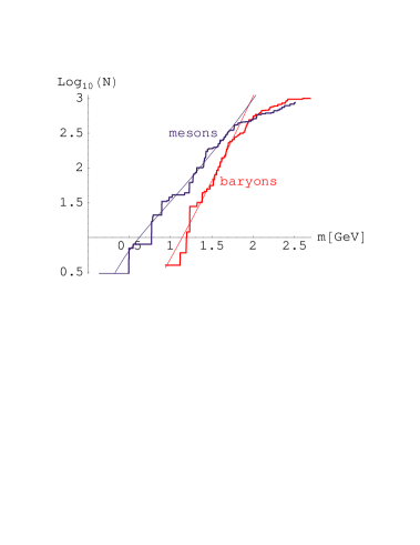
In Fig. 1 we compare the cumulants of the spectrum [4], defined as the number of states with mass lower than $m$. The experimental curve is

$$N_{{\rm exp}}(m)=\sum_{i}g_{i}\Theta(m-m_{i}),$$ (2)

where $g_{i}=(2J_{i}+1)(2I_{i}+1)$ is the spin-isospin degeneracy of the $i$th state, and $m_{i}$ is its mass. The theoretical curve corresponds to

$$N_{{\rm theor}}(m)=\int_{0}^{m}\rho_{{\rm theor}}(m^{\prime})dm^{\prime},$$ (3)

where

$$\rho_{{\rm theor}}(m)=f(m)\exp(m/T),$$ (4)

with $f(m)$ denoting a slowly-varying function. A typical choice [3, 8], used in the plot of Fig. 1, is

$$f(m)=A/(m^{2}+(500{\rm MeV})^{2})^{5/4}.$$ (5)

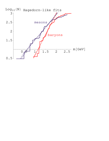
Parameters $T_{H}$ and $A$ are obtained with the least-square fit to $\log N_{{\rm theor}}$, made over the range up to $m=1.8{\rm GeV}$, and skipping the lightest particle in the set. Other choices of $f(m)$ give fits of similar quality (see Fig. 2). A striking feature of Fig. 1 is the linearity of $\log N$ starting at very low $m$, and extending till $m\sim 1.8{\rm GeV}$. Clearly, this shows that (1) is valid in the range of available data. However, the slopes in Fig. 1 are different for mesons and baryons. For the assumed $f(m)$ of Eq. (5) we get

$$T_{{\rm meson}}=195{\rm MeV},\;\;\;T_{{\rm baryon}}=141{\rm MeV}.$$ (6)

This means that $T_{{\rm meson}}>T_{{\rm baryon}}$, and the inequality is substantial! Although it has been known to researchers in the field of hadron spectroscopy that the baryons multiply more rapidly than mesons [9], to our knowledge this fact has not been presented as vividly as in Fig. 1. To emphasize the strength of the effect we note that in order to make the meson line parallel to the baryon line, we would have to aggregate $\sim 500$ additional meson states up to $m=1.8$MeV as compared to the present number of $\sim 400$.

2.2 Are we asymptotic?

An important question is whether the presently available range of masses is asymptotic in view of Eq. (1). The answer is no! This is how we can look at this question quantitatively.

Formula	$m_{0}$	$T_{\rm{mes}}$	$T_{\rm{bar}}$	$\sigma^{2}_{\rm{mes}}$	$\sigma^{2}_{\rm{bar}}$
	MeV	MeV	MeV
$\frac{A}{(m^{2}+m_{0}^{2})^{5/4}}\exp({m\over T})$	500	195	141	0.016	0.015
- - -	1000	228	152	0.014	0.015
- - -	250	177	136	0.025	0.015
$\frac{A}{(m+m_{0})^{5/2}}\exp(\frac{m}{T})$	1000	223	154	0.015	0.015
$A\exp(\frac{m}{T})$		311	186	0.014	0.015
$\frac{A}{m}I_{2}(\frac{m}{T})$		249	157	0.014	0.015

Table 1: Various Hagedorn-like fits. Rows 1-4 use formulas of Ref. citeSBM1, row 5 uses a simple exponent, and row 6 uses the scalar string model of Ref. [10]. The last two column display the mean suared deviation for the meson and baryon case, respectively.

Consider the generic form of the spectrum of Eq. (4). We can rewrite it as

$$f(m)e^{m/T}=e^{\log f(m)+m/T}\simeq e^{\log[f(\overline{m})+f^{\prime}(\overline{m})\Delta m]+(\overline{m}+\Delta m)/T}=$$

$${\rm const}\;e^{\left(\frac{1}{T}+\frac{f^{\prime}(\overline{m})}{f(\overline{m})}\right)\Delta m}={\rm const}\;e^{\frac{\Delta m}{T_{{\rm eff}}}},$$

where $m=\overline{m}+\Delta m$, and in the range of data $\overline{m}\sim 1$GeV. We have defined $T_{{\rm eff}}$ as the effective Hagedorn temperature in the (non-asymptotic) region around $\overline{m}$. The value of $T_{{\rm eff}}$ follows directly from the data. We have, according to Eq. (2.2),

$$\frac{1}{T}=\frac{1}{T_{{\rm eff.}}}-\frac{f^{\prime}(\overline{m})}{f(\overline{m})}.$$ (7)

The following statements are obvious:

• since $f^{\prime}(\overline{m})<0$, $T<T_{{\rm eff}}$,

• only at $m\to\infty$ we have $T=T_{{\rm eff}}$. In the region of data we find significant differences between $T$ and $T_{{\rm eff}}$.

Here is a numerical example. Consider

$$f(m)=\frac{A}{(m^{2}+m_{0}^{2})^{5/4}},$$ (8)

which leads to

$$\frac{1}{T}=\frac{1}{T_{{\rm eff.}}}+\frac{5}{2}\frac{\overline{m}}{(\overline{m}^{2}+m_{0}^{2})}$$ (9)

Now we take $m_{0}=0.5$GeV and $\overline{m}=1$GeV and find

• for mesons: $T_{{\rm eff}}=311$MeV, $T=192$MeV (exact fit: 195MeV)

• for baryons: $T_{{\rm eff}}=186$MeV, $T=136$MeV (exact fit: 141MeV)

We conclude that only in the asymptotic region, $m>>m_{0}$, the choice of $f(m)$ is not important. In the region of presently-available data $f(m)$ matters very much for the extracted values of the Hagedorn temperature. This simply means that we need a theory in order to make quantitative statements!

The numerical parameters obtained from various choices of the function $f(m)$ are collected in Table 1. Figure 2 shows the fits corresponding to the rows 1, 4, 5 and 6 of Table 1. Note the fits are very close to each other and the theoretical curves are virtually indistinguishable in the region of data. In view of the above discussion it makes little sense to treat the Hagedorn temperature as an absolute parameter and to quote its value without specifying the model that yields the function $f(m)$.

2.3 Flavor universality

Fig. 3: Strange vs. non-strange mesons (a), and baryons (b).

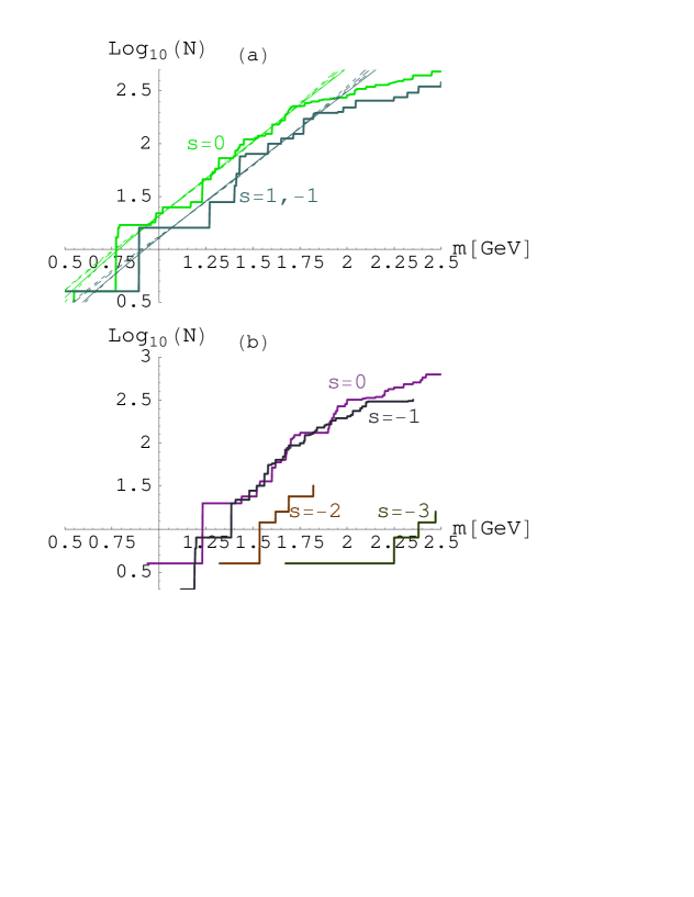
In Fig. 3 we show the cumulants of particle spectra of a given value of strangeness. We can clearly see that the slopes in the figure do not depend on strangeness. The meson plot includes various Hagedorn fits of Fig. 2. The two sets of lines are displaced in the $m$ variable by roughly $150$MeV, which is the difference of the masses on the strange and non-strange quarks. The conclusion here is that the addition of the strange quark mass has no effect on the rate of growth of the number of states with $m$. Certainly, we are rediscovering the $SU(3)$ flavor symmetry here!

2.4 Plot in the exponential variable

Fig. 4: Cumulants of the meson and baryon spectra plotted in exponential variables.

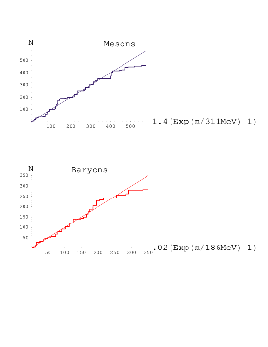
We end the experimental part of this talk by showing the same information as in Fig. 1, but instead of using logarithmic units on the vertical axes, we take exponential units on the horizontal axis. More precisely, we take the fit to the spectrum with of the form with the simple exponent (row 5 in Table 1), which leads to the cumulant $N(m)=AT(\exp(m/T)-1)$, where the values of $A$ and $T$ result from the least-square fit. Next, we define the variable $y=AT(\exp(m/T)-1)$ and plot the cumulants as functions of $y$. Note that the $A$ and $T$ parameters are different for mesons and baryons. Again, the linearity of data in the figure is striking. It starts at basically $m=0$, and extends to $m\sim 1.8$GeV. The advantage of the plot in Fig. 4 to that of Fig. 1 is that now the steps in the experimental cumulant are of a similar size independently of $m$.

We conclude this section by stating that the exponential growth of hadronic spectra in the region of $m$ up to about 1.8GeV, with $T_{{\rm mes}}>T_{{\rm bar}}$, is an experimental fact.

3 Theory

We are faced with two basic theoretical questions:

1. Why is the spectrum of resonances exponential?

2. Why do mesons and baryons behave so differently?

Concerning the first question, let us stress that it is not at all easy to get an exponentially rising spectrum of resonances. Take the simplistic harmonic-oscillator model, whose density of states grows as $m^{d-1}$, with $d$ denoting the number of dimensions. For mesons there is one relative coordinate, hence $\rho\sim m^{2}$, whereas the two relative coordinates in the baryon give $\rho\sim$ $m^{5}$. Weaker-growing potentials lead to a faster growth of the number of states, but fall short of the behavior (1). We know of three approaches yielding behavior (1), both involving combinatorics of infinitely-many degrees of freedom. These are the Statistical Bootstrap Model [1, 2, 3, 11], Bag Models [12, 13, 14], and Dual String Models [7]. The first two, however, lead to the same rate of growth for the mesons and baryons. Statistical Bootstrap Models are discussed in Sec. 3.1. In Bag Models [12, 13, 14] the exponential growth of the spectrum is associated with the melting out of the vacuum around the bag when the hadron is being excited. Since the scales in the Bag Model are practically the same for the meson and the baryon (the size scales as the number of constituents to the power $1/4$), the Bag Models are not capable of answering question 2. On the other hand, the Dual String Models [7] is offer a natural explanation of questions 1 and 2. This has already been pointed out in Ref. [6].

3.1 Statistical Bootstrap Models

Statistical bootstrap models [1, 3, 11] form particles from clusters of particles, and employ the principle of self-similarity. The simplest, “generic”, bootstrap equation has the form

$$\rho(m)=\delta(m-m_{0})+\sum_{n=2}^{\infty}\frac{1}{n!}\int_{0}^{\infty}dm_{1}...dm_{n}\times\delta(m-\sum_{i=1}^{n}m_{i})\rho(m_{1})...\rho(m_{n}),$$ (10)

where $\rho(m)$ is the particle spectrum (here, for a moment, mesons and baryons are not distinguished). Equation (10) can be nicely solved with help of Laplace transforms [1, 3, 15], yielding the asymptotic solution $\rho(m)\sim\exp(m/T)$, with $T={m_{0}}/{\log(-\log\frac{4}{e})}$. More complicated bootstrap equations involve integration over momenta, more degrees of freedom, different combinatorial factors [3], however, irrespectively of these details, they always lead to an exponentially growing spectrum. It can be shown, following e.g. the steps of Ref. [16], that the model leads to equal Hagedorn temperatures for mesons and for baryons. This is quite obvious. Since baryons are formed by attaching mesons to the “input” baryon, the baryon spectrum grows at exactly the same rate as the meson spectrum. Specific calculations confirm this simple observation. Thus the bootstrap idea is not capable of explaining the different behavior of mesons and baryons in Fig. 1.

3.2 Dual String models

Fig. 5: Meson and baryon string configurations.

The Dual String models [7] also date back to pre-QCD times. Their greatest success is a natural explanation of the Regge trajectories – a basic experimental fact which remain a serious problem for other approaches. Similarly to the bootstrap models, the Dual String Models lead to exponentially-growing spectra, but they do give the demanded effect of $T_{{\rm meson}}>T_{{\rm baryon}}$, at least at asymptotic masses [6].

Let us analyze mesons first. The particle spectrum is generated by the harmonic-oscillator operator describing vibrations of the string,

$$N=\sum_{k=1}^{\infty}\sum_{\mu=1}^{D}ka_{k,\mu}^{\dagger}a_{k,\mu},$$ (11)

where $k$ labels the modes and $\mu$ labels additional degeneracy, related to the number of dimensions [7]. Eigenvalues of $N$ are composed in order to get the square of mass of the meson, according to the Regge formula

$$\alpha^{\prime}m^{2}-\alpha_{0}=n,$$ (12)

where $\alpha^{\prime}\sim 1{\rm GeV}^{-2}$ is the Regge slope, and $\alpha_{0}\approx 0$ is the intercept. Here is an example: take $n=5$. The value 5 can be formed by taking the $k=5$ eigenvalue of $N$ (this is the leading Regge trajectory, with a maximum angular momentum), but we can also obtain the same $m^{2}$ by exciting one $k=4$ and one $k=1$ mode, alternatively $k=3$ and $k=2$ modes, and so on. The number of possibilities corresponds to partitioning the number $5$ into natural components: 5, 4+1, 3+2, 3+1+1, 2+2+1, 2+1+1+1, 1+1+1+1+1. Here we have 7 possibilities, but the number of partitions grows very fast with $n$. Partitions with more than one component describe the sub-leading Regge trajectories. With $D$ degrees of freedom each component can come in $D$ different species. Let us denote the number of partitions in our problem as $P_{D}(n)$. For large $n$ the asymptotic formula for partitio numerorum leads to the exponential spectrum according to the formula [17, 7].

$$\rho(m)=2\alpha^{\prime}mP_{D}(n),\quad P_{D}(n)\simeq\sqrt{\frac{1}{2n}}\left(\frac{D}{24n}\right)^{\frac{D+1}{4}}\exp\left(2\pi\sqrt{\frac{Dn}{6}}\right),$$ (13)

where $n=\alpha^{\prime}m^{2}$. We can now read-off the mesonic Hagedorn temperature:

$$T_{{\rm meson}}=\frac{1}{2\pi}\sqrt{\frac{6}{D\alpha^{\prime}}}.$$ (14)

Fig. 6: Predicions of the scalar string model of Ref. [10], with $D=6$.

Now the baryons: the “Mercedes-Benz” string configuration for the baryon is shown in Fig. 5. The three strings vibrate independently, and the corresponding vibration operators, $N$, add up. Consequently, their eigenvalues $n_{1}$, $n_{2}$, and $n_{3}$ add up. Thus we simply have a partition problem with $3$ times more degrees of freedom than in the meson. The replacement $D\rightarrow 3D$ in (13) leads immediately to

$$T_{{\rm baryon}}=\frac{1}{2\pi}\sqrt{\frac{2}{D\alpha^{\prime}}},$$ (15)

such that

$$T_{{\rm meson}}/T_{{\rm baryon}}=\sqrt{3}.$$ (16)

We stress that the presented picture is fully consistent with the Regge phenomenology. The leading Regge trajectory for baryons is generated by the excitation of a single string, i.e. two out of three numbers $n_{i}$ vanish (this is the quark-diquark configuration). The subleading trajectories for baryons come in a much larger degeneracy than for mesons, due to more combinatorial possibilities. The slopes of the meson and baryon trajectories are universal, and given by $\alpha^{\prime}$. We stress that the “number-of-strings” mechanism described above is asymptotic. Thus, there is a problem in applying string models to the experimentally accessible range of $m$. This range is not asymptotic enough to use Eq. (13). From the Regge formula (12) we find immediately that for $m$ in the range $1-2$GeV the values of $n$ lie between $1$ and $4$, hence $n$ is not large enough to justify the form (13).

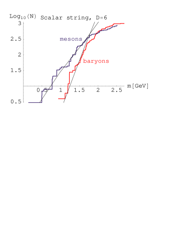
One can do better by using an improved asymptotic formula, derived in Ref. [10]. The results obtained in the scalar string model [10] are displayed in Fig. 6. Here the formula for the meson spectrum is

$$\rho_{{\rm mes}}(m)=36\times\rho_{{\em scalar}}(m),\;\;\;\rho_{{\em scalar}}(m)=\frac{2\alpha^{\prime}}{(4\pi\alpha^{\prime}mT_{{\rm mes}})^{\nu}}{mI_{\nu}(\frac{m}{T_{{\rm mes}}})},$$ (17)

where $I_{2}$ is a modified Bessel function, $T_{{\rm mes}}$ is the meson Hagedorn temperature (the only adjustable parameter here), and $\nu=1+D/2$, with $D$ denoting the number of transverse dimensions. The factor of $36=6\times 6$ is just the spin-flavor degeneracy of the $\overline{q}q$ configuration [10]. For the baryons we fold the three scalar-string densities, $\rho_{{\em scalar}}(m)$. We use $56$ (rather than $36$) copies of the string, which is the degeneracy of the baryon multiplet in the ground state. We notice good agreement with data in Fig. 6, for $D=6$. Note that both curves are fitted with only one parameter, $T_{{\rm mes}}$. For lower values of $D$ one can fit the mesons equally well, but too many baryon states are predicted.

3.3 Exotics as dual strings

During this workshop we have heard many talks on hadron exotics. If an exotic is a multi-string configuration, e.g. as in Fig. 7, then the corresponding spectrum will grow exponentially with the Hagedorn temperature inversely proportional to the square root of the number of strings. For instance, $T_{q\overline{q}q\overline{q}}=\frac{1}{\sqrt{5}}T_{{\rm meson}}$. This is reminiscent of the effect described in Ref. [18]. For the glueballs, described by the closed string in Fig. (7), we get $T_{G}=T_{{\rm meson}}$.

Fig. 7: $\overline{q}q\overline{q}q$ and glueball configurations.

Thus, according to the string model, the $q\overline{q}q\overline{q}$ grow more rapidly than non-exotic mesons and baryons, and glueballs grow at the same rate as mesons.

4 Other approaches

In the remaining part of this talk we will, in a sense, work against our results presented in previous sections, where have we argued that the plots of Fig. 1 are linear, and offered an explanation of the difference between the mesonic and baryonic Hagedorn temperatures within the Dual String Models.

What if the experimental plots of Fig. 1 are not really linear, and the effect of bending down of the curves at higher masses is physical, rather than due to incomplete experiments? Below we will show alternative descriptions which do not comply to Eq. (1), but nevertheless reproduce the present data at least as good as the Hagedorn-like fits.

4.1 Compound hadrons

In the statistical model of nuclear reactions one uses the compound-nucleus model [19, 20]. In this model the density of states grows at large excitation energies, $E^{*}$, according to the formula

$$\rho(E)\sim(E^{*})^{-5/4}e^{a\sqrt{E^{*}}},$$ (18)

where $a$ is a constant. Formula (18) can be derived within the Fermi gas model [20]. More generally, it can be derived in a model where the single-particle orbits are equally spaced. One then considers $1p1h$, $2p2h$, $3p3h$, etc., excitations and counts the number of states at a given excitation energy, $E^{*}$. Amusingly, this leads [21] to the partitio numerorum formula (13), but now the number $n$ has the interpretation $n=E^{*}/\Delta E$, with $\Delta E$ denoting the level spacing.

Fig. 8: Fits of the Compound Hadron Model, Eq. (19).

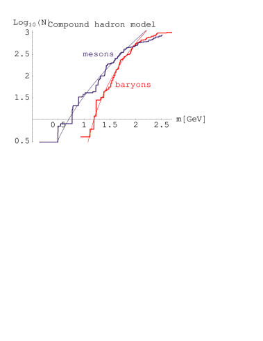
We now use the following Compound-Hadron-Model formula for the mass spectra:

$$\rho(m)=\frac{A\Theta(m-m_{0})\exp\left(2\pi\sqrt{\frac{\left(m-m_{0}\right)}{6\Delta E}}\right)}{\left(\left(m-m_{0}\right)^{2}+(0.5{\rm GeV})^{2}\right)^{5/8}},$$ (19)

where $A$ is a constant, $m_{0}$ is the ground-state mass, and $\Delta E$ is the average level spacing. The constant $0.5$GeV in the denominator has been introduced ad hoc, similarly as in Eq. (5), in order for the formula to make sense at $m\rightarrow m_{0}$. Asymptotically, the power of $m$ multiplying the exponent is $-5/4$, as in Eq. (18).

The underlying physical picture behind compound hadrons is as follows: hadrons are bound objects of constituents (quarks, gluons, pions). The Fock space contains a ground state, and excitations on top of it. In the case of the compound nucleus these elementary excitations are $1p1h$, $2p2h$, $3p3h,$ etc. states. In the case of hadrons they are formed of $q\bar{q}$ and gluon excitations, e.g. for mesons we have $q\bar{q}$, $q\bar{q}g$, $qq\bar{q}\bar{q}$, $q\bar{q}gg$, etc. We can form the excitation energy (hadron mass) by differently composing elementary excitations. This bring us to the above-described combinatorial problem [21]. It seems reasonable to take zero ground-state energy for mesons, $m_{0}^{{\rm mes}}=0$, since they are excitations on top of the vacuum. For baryons we take $m_{0}^{{\rm bar}}=900$MeV, which is the mass of the nucleon. The quantity $\Delta E$ is treated as a model parameter and is fitted to data.

The results of the compound-hadron-model fit, Eq. (19), are shown in Fig. 8. The curves are slightly bent down, compared to the Hagedorn-like fits of Figs. 1,2, which is caused by the square root in the exponent of Eq. (19). But the fits are at least as good, or even better when the fit region is extended to $m=2$GeV. Numerically, the least-square fit for $m$ up to 1.8GeV gives $\Delta E^{{\rm mes}}=100$MeV for mesons, and $\Delta E^{{\rm bar}}=106$MeV for baryons. The proximity of these numbers shows that the scales for mesons and baryons are similar, as should be the case.

The obtained values for $\Delta E^{{\rm mes}}$ mean that the corresponding $n$ at $m=1.8$GeV is around $18$ for mesons and $9$ for baryons. Such values of $n$ are sufficiently large to justify the use of the asymptotic formulas.

4.2 Combinatorial saturation and the light-flavor-desert hypothesis

Fig. 9: Experimental cumulants and the predicions of the quark model of Ref. [22, 23], as counted in Ref. [9], indicated by dots.

There is a possibility of an interesting effect we wish to point out. It is natural to expect that a bound hadronic system has an upper limit for the excitation energy. It is helpful to think here of bags of finite depth. Thus, in constructing the single-particle Fock space for bound objects we should have a limited number of quanta to our disposal. If such a limit is put into the Compound Hadron Model, it will result in a maximum number of states that can possibly be formed out of light quarks [5]. We can call it the “light-flavor-desert hypothesis”: above a certain mass there are no more light-flavor resonances. Certainly, this is tangential to the conventional wisdom that the Regge trajectories should continue indefinitely. Note, however, that infinite Regge trajectories have recently been challenged by Brisudová, Burakovsky and Goldman, who claim that they should stop around $m\sim 2.7$GeV. Amusingly, this is consistent with the presently-available data. The cumulants if Fig. 1 flatten-out in that region.

4.3 Quark models

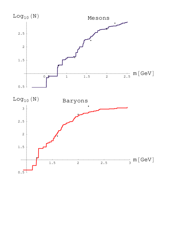
Many talk in this workshop were devoted to variants of the quark model. Here we present the result of counting of states in the model of Refs. [22, 23], as made by Freund and Rosner [9].

When we look at Fig. 9, we again see good agreement in the predicted and experimental number of states. This is not at all surprising, since the quark model is designed to fit the data “state by state” in the low-mass regime. As for other approaches, spectra at higher $m$ would be needed to verify the predictions.

5 Final remarks

There are many fundamental questions which should be cleared when more experimental data on hadron resonances are available: Is the Hagedorn hypothesis of exponentially-growing spectra indeed correct, or is the growth weaker at higher masses? Do the Regge trajectories continue for ever, or stop? Consequently, is there a light-flavor desert above a certain mass? Are there exotic states, if so, at what rate do they grow?… Certainly, the spectrum above 2GeV may reveal many answers and help us to verify various models and approaches.

However, even the presently-available spectrum allows for interesting speculations. Recall the remarks made here by Leonid Glozman, concerning the parity doublets in the $N$ and $\Delta$ spectra above $2$GeV [24]. Almost all states in that region can be paired, and such a regularity suggests that the data in that region may be complete! This, in turn, indicates that the bending down of the cumulants in Fig. 1 may be a physical, rather than experimental effect.

Another important aspect, not touched in this talk, are the thermodynamical implications of the presence of two distinct Hagedorn temperatures for the phenomenology of heavy-ion collisions, transition to quark-gluon plasma, etc. This will be discussed in [21].

The author thanks Keith R. Dienes for many profitable e-mail discussions on the issues of hadron spectra in string models, as well as to Andrzej Białas, Andrzej Horzela, Jan Kwieciński, and Kacper Zalewski for numerous useful comments and encouragement.

REFERENCES

- [1] R. Hagedorn, Suppl. Nuovo Cim. 3 (1965) 147
- [2] R. Hagedorn, CERN preprint No. CERN 71-12 (1971), and references therein
- [3] R. Hagedorn, CERN preprint No. CERN-TH.7190/94 (1994), and references therein
- [4] Particle Data Group, Eur. Phys. J. C 3 (1998) 1
- [5] W. Broniowski and W. Florkowski, INP Cracow preprint No. 1843/PH (2000), hep-ph//0004104
- [6] W. Broniowski, talk presented at Meson 2000, 19-23 May 2000, Cracow, hep-ph//0006020
- [7] in Dual Theory, Vol. 1 of Physics Reports reprint book series, edited by M. Jacob (North Holland, Amsterdam, 1974)
- [8] R. Hagedorn and J. Ranft, Suppl. Nuovo Cim. 6 (1968) 169
- [9] G. O. Freund and J. L. Rosner, Phys. Rev. Lett. 68 (1992) 765
- [10] K. R. Dienes and J.-R. Cudell, Phys. Rev. Lett. 72 (1994) 187
- [11] S. Frautschi, Phys. Rev. D 3 (1971) 2821
- [12] A. Chodos, R. L. Jaffe, K. Johnson, C. B. Thorn, and V. F. Weisskopf, Phys. Rev. D 9 (1974) 3471
- [13] J. Kapusta, Nucl. Phys. B 196 (1982) 1
- [14] R. Gagnon and L. Marleau, Phys. Rev. D 35 (1987) 910
- [15] J. Yellin, Nucl. Phys. B 52 (1973) 583
- [16] W. Nahm, Nucl. Phys. B 45 (1972) 525
- [17] G. H. Hardy and S. S. Ramanujan, Proc. London Math. Soc. 17 (1918) 76
- [18] J.-R. Cudell and K. R. Dienes, Phys. Rev. Lett. 69 (1992) 1324
- [19] E. Vogt, in Advances in Nuclear Physics, edited by M. Baranger and E. Vogt (Plenum Press, New York, 1968), Vol. 1, p. 261
- [20] A. Bohr and B. R. Mottelson, Nuclear Structure (Benjamin, Reading, Massachussetts, 1969), Vol. 1
- [21] W. Broniowski, W. Florkowski, and P. Żenczykowski, to be published
- [22] S. Godfrey and N. Isgur, Phys. Rev. D 32 (1985) 189
- [23] S. Capstick and N. Isgur, Phys. Rev. D 34 (1986) 2809
- [24] L. Y. Glozman, Nucl. Phys. B 475 (2000) 329