$b\rightarrow s\tau^{+}\tau^{-}$ decay in the two Higgs doublet model with flavor changing neutral currents

Abstract

We study the decay width and forward-backward asymmetry of the lepton pair for the inclusive decay $b\rightarrow s\tau^{+}\tau^{-}$ in the two Higgs doublet model with three level flavor changing neutral currents (model III) and analyse the dependencies of these quantities on the model III parameters, including the leading order QCD corrections. We found that there is a considerable enhancement in the decay width and neutral Higgs effects are detectable for large values of the parameter $\bar{\xi}_{N,\tau\tau}^{D}$.

1 Introduction

Currently, there is an impressive experimental effort for studying rare B-meson decays at SLAC (BaBar), KEK (BELLE), B-Factories, DESY (HERA-B) since these decays are rich phenomenologically. They are induced by flavor changing neutral currents (FCNC) at loop level in the Standard model (SM) and with the forthcoming experiments, it would be possible to test the flavour sector of the SM in a high precision, as well as to reveal the physics beyond, such as two Higgs Doublet model (2HDM), Minimal Supersymmetric extension of the SM (MSSM) [1], etc.

Among the rare B decays, $B\rightarrow K^{*}l^{+}l^{-}$ process has received a great interest since the SM prediction for its branching ratio ($Br$) is large enough to be measured in the near future. This decay is induced by $b\rightarrow sl^{+}l^{-}$ transition at the quark level and in the literature it has been investigated extensively for $l=e,\mu$ in the SM, 2HDM and MSSM [2]- [15]. When $l=e,\mu$, the neutral Higgs boson (NHB) effects are safely neglected in the 2HDM because they enter in the expressions with the factor $m_{e(\mu)}/m_{W}$. However, for $l=\tau$, this factor is not negligible and NHB effects can give important contribution. In [16, 17], $B\rightarrow X_{s}\tau^{+}\tau^{-}$ process was studied in the 2HDM and it was shown that NHB effects are sizable for large values of $tan\beta$.

In this work, we study the $b\rightarrow s\tau^{+}\tau^{-}$ decay in the general 2HDM , so-called model III. We include NHB effects and make the full calculation using the on-shell renormalization prescription. We investigate the dependencies of the differential decay width $d\Gamma/ds$ and the decay width $\Gamma$ on the scale invariant lepton mass square ”$s$” and some model III parameters, namely $m_{H^{\pm}}$, $\bar{\xi}_{N,bb}^{D}$ and $\bar{\xi}_{N,\tau\tau}^{D}$. Further, we calculate the differential (direct) forward-backward asymmetry $A_{FB}(s)$ ($A_{FB}$) of the lepton pair in terms of the above parameters. We show that a large enhancement is possible in the decay width of the process $b\rightarrow s\tau^{+}\tau^{-}$ for some values of the model III parameters and NHB effects become considerable for large values of $\bar{\xi}_{N,\tau\tau}^{D}$.

The paper is organized as follows: In Section 2, we present the leading order (LO) QCD corrected effective Hamiltonian and the corresponding matrix element for the inclusive $b\rightarrow s\tau^{+}\tau^{-}$ decay. Further, we give the expression for $A_{FB}(s)$ and $A_{FB}$ of the lepton pair. Section 3 is devoted to the analysis of the new Wilson coefficients coming from the NHB effects and the dependencies of $d\Gamma/ds$, $\Gamma$, $A_{FB}(s)$ and $A_{FB}$ on the the Yukawa couplings $\bar{\xi}_{N,bb}^{D}$, $\bar{\xi}_{N,\tau\tau}^{D}$, the charged Higgs mass $m_{H^{\pm}}$, the parameter s and to the discussion of our results. In Appendices, we give the explicit forms of the operators appearing in the effective Hamiltonian and the corresponding Wilson coefficients.

2 The inclusive $b\rightarrow s\tau^{+}\tau^{-}$ decay in the model III

Model III (2HDM) permits the flavour changing neutral currents in the tree level and the prize is various new parameters, i.e. Yukawa couplings. These couplings are responsible for the interaction of quarks and leptons with gauge bosons, namely, the Yukawa interaction and in this general case it reads as

$${\cal{L}}_{Y}=\eta^{U}_{ij}\bar{Q}_{iL}\tilde{\phi_{1}}U_{jR}+\eta^{D}_{ij}\bar{Q}_{iL}\phi_{1}D_{jR}+\xi^{U}_{ij}\bar{Q}_{iL}\tilde{\phi_{2}}U_{jR}+\xi^{D}_{ij}\bar{Q}_{iL}\phi_{2}D_{jR}+h.c.\,\,\,,$$ (1)

where $L$ and $R$ denote chiral projections $L(R)=1/2(1\mp\gamma_{5})$, $\phi_{k}$, for $k=1,2$, are the two scalar doublets, $Q_{iL}$ are quark and lepton doublets, $U_{jR}$, $D_{jR}$ are the corresponding singlets, $\eta^{U,D}_{ij}$, and $\xi^{U,D}_{ij}$ are the matrices of the Yukawa couplings. The Flavor changing (FC) part of the interaction is given by

$${\cal{L}}_{Y,FC}=\xi^{U}_{ij}\bar{Q}_{iL}\tilde{\phi_{2}}U_{jR}+\xi^{D}_{ij}\bar{Q}_{iL}\phi_{2}D_{jR}+h.c.\,\,.$$ (2)

The choice of $\phi_{1}$ and $\phi_{2}$

$$\phi_{1}=\frac{1}{\sqrt{2}}\left[\left(\begin{array}[]{c c}0\\ v+H^{0}\end{array}\right)\;+\left(\begin{array}[]{c c}\sqrt{2}\chi^{+}\\ i\chi^{0}\end{array}\right)\right]\,;\phi_{2}=\frac{1}{\sqrt{2}}\left(\begin{array}[]{c c}\sqrt{2}H^{+}\\ H_{1}+iH_{2}\end{array}\right)\,\,.$$ (9)

with the vacuum expectation values,

$$<\phi_{1}>=\frac{1}{\sqrt{2}}\left(\begin{array}[]{c c}0\\ v\end{array}\right)\,\,;<\phi_{2}>=0\,\,,$$ (12)

ensures decoupling of the SM and beyond. In eq.(2) the couplings $\xi^{U,D}$ for the FC charged interactions are

$$\xi^{U}_{ch} = \xi_{neutral}\,\,V_{CKM}\,\,,$$

$$\xi^{D}_{ch} = V_{CKM}\,\,\xi_{neutral}\,\,,$$ (13)

where $\xi^{U,D}_{neutral}$ is defined by the expression

$$\xi^{U,D}_{N}=(V_{L}^{U,D})^{-1}\xi^{U,D}V_{R}^{U,D}\,\,.$$ (14)

Here the charged couplings appear as linear combinations of neutral couplings multiplied by $V_{CKM}$ matrix elements (see [18] for details).

Now we would like to start with the calculation of the matrix element for the inclusive $b\rightarrow s\tau^{+}\tau^{-}$ decay. The procedure is to integrate out the heavy degrees of freedom, namely $t$ quark, $W^{\pm},H^{\pm},H^{0},H_{1}$, and $H_{2}$ bosons in the present case and obtain the effective theory. Here $H^{\pm}$ denote charged, $H^{0}$, $H_{1}$ and $H_{2}$ denote neutral Higgs bosons. Note that $H_{1}$ and $H_{2}$ are the same as the mass eigenstates $h^{0}$ and $A^{0}$ in the model III respectively, due to the choice given by eq. (9). The QCD corrections are done through matching the full theory with the effective low energy one at the high scale $\mu=m_{W}$ and evaluating the Wilson coefficients from $m_{W}$ down to the lower scale $\mu\sim O(m_{b})$. In the model III (similar to the models I and II, 2HDM) neutral Higgs particles bring new contributions to the matrix element of the process $b\rightarrow s\tau^{+}\tau^{-}$ (see eq.(31)) since they enter in the expressions with the mass of $\tau$ lepton or related Yukawa coupling $\bar{\xi}^{D}_{N,\tau\tau}$. As being different from the model I and II, in the model III, there exist additional operators which are the flipped chirality partners of the former ones. However, the effects of the latter are negligible since the corresponding Wilson coefficients are small due to the discussion given in section 3. Therefore, the effective Hamiltonian relevant for the process $b\rightarrow s\tau^{+}\tau^{-}$ is

$${\cal{H}}_{eff}=-4\frac{G_{F}}{\sqrt{2}}V_{tb}V^{*}_{ts}\left\{\sum_{i}C_{i}(\mu)O_{i}(\mu)+\sum_{i}C_{Q_{i}}(\mu)Q_{i}(\mu)\right\}\,\,,$$ (15)

where $O_{i}$ are current-current ($i=1,2$), penguin ($i=3,...,6$), magnetic penguin ($i=7,8$) and semileptonic ($i=9,10$) operators. Here, $C_{i}(\mu)$ are Wilson coefficients normalized at the scale $\mu$ and given in Appendix B. The additional operators $Q_{i}(i=1,..,10)$ are due to the NHB exchange diagrams and $C_{Q_{i}}(\mu)$ are their Wilson coefficients (see Appendices A and B) .

During the calculations of NHB contributions, we use the on-shell renormalization scheme to overcome the logarithmic divergences. Taking the vertex function

$$\Gamma_{neutr}^{Ren}(p^{2})=\Gamma_{neutr}^{0}(p^{2})+\Gamma_{neutr}^{C},$$ (16)

and using the renormalization condition

$$\Gamma_{neutr}^{Ren}(p^{2}=m^{2}_{neutr})=0,$$ (17)

we get the counter terms and then calculate $\Gamma_{neutr}^{Ren}(p^{2})$ . Here the phrase $neutr$ denotes the neutral Higgs bosons, $H^{0}$, $h^{0}$ and $A^{0}$ and $p$ is the momentum transfer.

Now we give the QCD corrected amplitude for the inclusive $b\rightarrow s\tau^{+}\tau^{-}$ decay in the model III,

$${\cal M} = \frac{\alpha G_{F}}{\sqrt{2}\,\pi}V_{tb}V_{ts}^{*}\Bigg{\{}C_{9}^{eff}(\bar{s}\gamma_{\mu}P_{L}b)\,\bar{\tau}\gamma^{\mu}\tau+C_{10}(\bar{s}\gamma_{\mu}P_{L}b)\,\bar{\tau}\gamma^{\mu}\gamma_{5}\tau$$ (18)

$$- 2C_{7}\frac{m_{b}}{p^{2}}(\bar{s}i\sigma_{\mu\nu}p^{\nu}P_{R}b)\bar{\tau}\gamma^{\mu}\tau+C_{Q_{1}}(\bar{s}P_{R}b)\bar{\tau}\tau+C_{Q_{2}}(\bar{s}P_{R}b)\bar{\tau}\gamma_{5}\tau\Bigg{\}}~{}.$$

Using Eq.(18), the differential decay rate reads as

$$\frac{d\Gamma(b\rightarrow s\tau^{+}\tau^{-})}{ds} = Br(B\rightarrow X_{c}\ell\bar{\nu})\frac{\alpha^{2}}{4\pi^{2}f(m_{c}/m_{b})}(1-s)^{2}\left(1-\frac{4t^{2}}{s}\right)^{1/2}\frac{|V_{tb}V_{ts}^{*}|^{2}}{|V_{cb}|^{2}}D(s),$$ (19)

with

$$D(s) = |C^{eff}_{9}|^{2}\left(1+\frac{2t^{2}}{s}\right)(1+2s)+4|C_{7}|^{2}\left(1+\frac{2t^{2}}{s}\right)\left(1+\frac{2}{s}\right)+|C_{10}|^{2}\left[1+2s+\frac{2t^{2}}{s}(1-4s)\right]$$ (20)

$$+ 12Re(C_{7}C^{eff*}_{9})\left(1+\frac{2t^{2}}{s}\right)^{1/2}+\frac{3}{2}|C_{Q_{1}}|^{2}(s-4t^{2})+\frac{3}{2}|C_{Q_{2}}|^{2}+6Re(C_{10}C^{*}_{Q_{2}}),$$

where $s=p^{2}/m^{2}_{b}$, $t=m_{\tau}/m_{b}$, and $f(x)$ is the phase-space factor given by $f(x)=1-8x^{2}+8x^{6}-x^{8}-24x^{4}\log x$. In the above expression for the differential decay rate, we use the inclusive one since, in the heavy quark effective theory, the leading terms of inclusive decay rates of the heavy hadrons in the $1/m_{b}$ expansion becomes that of the free heavy quark, $b$-quark in our context.

The forward-backward asymmetry $A_{FB}$ of the lepton pair is another physical quantity which can be observed in the experiments and provide important clues to test the theoretical models used. Using the definition of differential $A_{FB}$

$$A_{FB}(s) = \frac{\int^{1}_{0}dz\frac{d\Gamma}{dsdz}-\int^{0}_{-1}dz\frac{d\Gamma}{dsdz}}{\int^{1}_{0}dz\frac{d\Gamma}{dsdz}+\int^{0}_{-1}dz\frac{d\Gamma}{dsdz}}$$ (21)

with $z=\cos\theta$, where $\theta$ is the angle between the momentum of the b-quark and that of $\tau^{+}$ in the center of mass frame of the dileptons $\tau^{+}\tau^{-}$, we get

$$A_{FB}(s)=\frac{E(s)}{D(s)}.$$ (22)

Here,

$$E(s) = Re(C^{eff}_{9}C^{*}_{10}s+2C_{7}C^{*}_{10}+C^{eff}_{9}C^{*}_{Q_{1}}t+2C_{7}C^{*}_{Q_{2}}t)$$ (23)

In addition, $A_{FB}$ can be defined as

$$A_{FB} = \frac{\int^{1}_{0}dz\frac{d\Gamma}{dz}-\int^{0}_{-1}dz\frac{d\Gamma}{dz}}{\Gamma}.$$ (24)

Note that during the calculations of $\Gamma$ and $A_{FB}$, we take into account only the second resonance for the LD effects coming from the reaction $b\rightarrow s\psi_{i}\rightarrow s\tau^{+}\tau^{-}$, where $i=1,..,6$ and divide the integration region for $s$ into two parts : $\frac{4m^{2}_{\tau}}{m^{2}_{b}}\leq s\leq\frac{(m_{\psi_{2}}-0.02)^{2}}{m^{2}_{b}}$ and $\frac{(m_{\psi_{2}}+0.02)^{2}}{m^{2}_{b}}\leq s\leq 1$, where $m_{\psi_{2}}=3.686\,GeV$ is the mass of the second resonance (see Appendix B for LD contributions).

3 Discussion

In the general 2HDM model, there are many free parameters, such as masses of charged and neutral Higgs bosons and the complex Yukawa couplings, $\xi_{ij}^{U,D}$, where $i,j$ are quark flavor indices and these parameters should be restricted using the experimental measurements. Usually, the stronger restrictions to the new couplings are obtained from the analysis of the $\Delta F=2$ (here $F=K,B_{d},D$) decays, the $\rho$ parameter and the $B\rightarrow X_{s}\gamma$ decay.

The neutral Higgs bosons $h_{0}$ and $A_{0}$ give contributions to the Wilson coefficient $C_{7}$ (see the appendix of [19] for details)

$$C_{7}^{h_{0}}(m_{W}) = (V_{tb}V^{*}_{ts})^{-1}\sum_{i=d,s,b}\bar{\xi}^{D}_{N,bi}\,\,\bar{\xi}^{D}_{N,is}\,\frac{Q_{i}}{8\,m_{i}\,m_{b}}\,\,,$$

$$C_{7}^{A_{0}}(m_{W}) = (V_{tb}V^{*}_{ts})^{-1}\sum_{i=d,s,b}\bar{\xi}^{D}_{N,bi}\,\,\bar{\xi}^{D}_{N,is}\,\frac{Q_{i}}{8\,m_{i}\,m_{b}}\,\,,$$ (25)

where $m_{i}$ and $Q_{i}$ are the masses and charges of the down quarks ($i=d,\,s,\,b$) respectively. These expressions show that the neutral Higgs bosons can give a large contribution to the coefficient $C_{7}$ which is in contradiction with the CLEO data [20],

$$Br(B\rightarrow X_{s}\gamma)=(3.15\pm 0.35\pm 0.32)\,10^{-4}\,\,.$$ (26)

Such dangerous terms can be removed by assuming that the couplings $\bar{\xi}^{D}_{N,is}$ ($i=d,s,b)$ and $\bar{\xi}^{D}_{N,db}$ are small enough to be able to reach the conditions $\bar{\xi}^{D}_{N,bb}\,\bar{\xi}^{D}_{N,is}<<1$ and $\bar{\xi}^{D}_{N,db}\,\bar{\xi}^{D}_{N,ds}<<1$. The discussion given above results in the following restrictions: $\bar{\xi}^{D}_{N,ib}\sim 0$ and $\bar{\xi}^{D}_{N,ij}\sim 0$, where the indices $i,j$ denote d and s quarks . Further using the constraints [21], coming from the $\Delta F=2$ mixing, the $\rho$ parameter [18], and the measurement by CLEO Collaboration eq. (26) we get the condition for $\bar{\xi}_{N,tc}$, $\bar{\xi}_{N,tc}<<\bar{\xi}^{U}_{N,tt}$ and take into account only the Yukawa couplings of quarks $\bar{\xi}^{U}_{N,tt}$ and $\bar{\xi}^{D}_{N,bb}$. As for $\bar{\xi}^{D}_{N,\tau\tau}$, we do not consider any constraint and increase this parameter to enhance the effects of neutral Higgs boson. (For further discussion about the restrictions of the model III parameters see [18, 21].)

In this section, we study the Wilson coefficients $C_{Q_{1}}(m_{b})$ and $C_{Q_{2}}(m_{b})$ coming from NHB effects and $s$, $\frac{\bar{\xi}^{D}_{N,bb}}{m_{b}}$ and $\bar{\xi}^{D}_{N,\tau\tau}$ dependencies of $d\Gamma/ds$ and $\Gamma$ for the inclusive decay $b\rightarrow s\tau^{+}\tau^{-}$, restricting $|C_{7}^{eff}|$ in the region $0.257\leq|C_{7}^{eff}|\leq 0.439$ due to the CLEO measurement, eq.(26) (see [21] for details). Our numerical calculations based on this restriction and throughout these calculations, we use the redefinition

$$\xi^{U,D}=\sqrt{\frac{4G_{F}}{\sqrt{2}}}\bar{\xi}^{U,D}\,\,,$$

we take the scale $\mu=m_{b}$ and use the input values given in Table (1).

Parameter	Value
$m_{\tau}$	$1.78$ (GeV)
$m_{c}$	$1.4$ (GeV)
$m_{b}$	$4.8$ (GeV)
$\alpha_{em}^{-1}$	129
$\lambda_{t}$	0.04
Br ($B\rightarrow X_{c}\ell\bar{\nu}$)	$0.103\pm 0.01$
$m_{t}$	$175$ (GeV)
$m_{W}$	$80.26$ (GeV)
$m_{Z}$	$91.19$ (GeV)
$\Lambda_{QCD}$	$0.225$ (GeV)
$\alpha_{s}(m_{Z})$	$0.117$
$sin\theta_{W}$	$0.2325$

Table 1: The values of the input parameters used in the numerical calculations.

In Fig. 1 (2), we present $m_{h^{0}}$ dependence of $C_{Q_{1}}(m_{b})$ for $C^{eff}_{7}>0$, $\bar{\xi}_{N,bb}^{D}=40\,m_{b}$ ($3\,m_{b}$), $\bar{\xi}_{N,\tau\tau}^{D}=5\,GeV$ in the case $|r_{tb}|=|\frac{\bar{\xi}_{N,tt}^{U}}{\bar{\xi}_{N,bb}^{D}}|<1\,(r_{tb}>1)$. Here $C_{Q_{1}}(m_{b})$ lies in the region bounded by solid lines. For $r_{tb}>1$, $m_{h^{0}}=80\,GeV$ and $m_{H^{0}}=100\,GeV$, the value of $C_{Q_{1}}(m_{b})$ changes between $0.020$ and $0.045$. However for $r_{tb}>1$, we get values, -9 and -12, more than two orders of magnitude larger compared to ones for $|r_{tb}|<1$, for the same value of $m_{h^{0}}$. Since $C_{Q_{1}}(m_{b})$ is directly proportional to $\bar{\xi}_{N,\tau\tau}^{D}$, its value may further increase with the increasing values of $\bar{\xi}_{N,\tau\tau}^{D}$. The corresponding 2HDM model II value of $C_{Q_{1}}(m_{b})$ can be extracted from [16] as beeing $\sim 0.4$ for large $\tan\beta$, $\tan\beta=25$.

For completeness, in Figs. 3 and  4, we give $m_{H^{0}}$ dependence of $C_{Q_{1}}(m_{b})$ and $m_{A^{0}}$ dependence of $C_{Q_{2}}(m_{b})$, for $C^{eff}_{7}>0$, $\bar{\xi}_{N,bb}^{D}=40\,m_{b}$, $\bar{\xi}_{N,\tau\tau}^{D}=5\,GeV$ in the case $|r_{tb}|<1$. As seen from Fig. 4, $m_{A_{0}}$ dependence of $C_{Q_{2}}(m_{b})$ is relatively weaker and for $m_{A_{0}}=80\,GeV$, $C_{Q_{2}}(m_{b})$ is between nearly $0.0284$ and $0.0291$. For $r_{tb}>1$, $C^{eff}_{7}>0$, $\bar{\xi}_{N,bb}^{D}=3\,m_{b}$ and $\bar{\xi}_{N,\tau\tau}^{D}=5\,GeV$, $C_{Q_{2}}(m_{b})$ reaches up to the value of $-0.38$. The 2HDM model II value of $|C_{Q_{2}}(m_{b})|$ is $\sim 0.4$ for $\tan\beta=25$ [16].

Now we continue the analysis of the measurable quantities $\Gamma$ and $A_{FB}$ of the process under consideration. In the following, we use the numerical values $m_{H^{0}}=150\,GeV$, $m_{h^{0}}=80\,GeV$ and $m_{A^{0}}=80\,GeV$ in our calculations.

In Fig. 5, we plot the differential $\Gamma$ of the decay $b\rightarrow s\tau^{+}\tau^{-}$ with respect to the parameter $s$ for $\bar{\xi}_{N,bb}^{D}=40\,m_{b}$, $\bar{\xi}_{N,\tau\tau}^{D}=1\,GeV$ and charged Higgs mass $m_{H^{\pm}}=400\,GeV$ in case of the ratio $|r_{tb}|<1$. Here the differential $\Gamma$ lies in the region bounded by dashed (small dashed) curves for $C_{7}^{eff}>0$ ($C_{7}^{eff}<0$). A small enhancement is possible especially for $C_{7}^{eff}>0$ case compared to the SM (solid curve). Further, the restriction region of the differential $\Gamma$ for model III becomes narrower with increasing or decreasing values of the parameter $s$. Fig. 6 is devoted the same dependence of the differential $\Gamma$ including the long distance (LD) effects. Here $C_{7}^{eff}<0$ case for model III almost coincides with the SM (solid curve). In case of the ratio $r_{tb}>1$, extremely large enhancement, 3 orders larger compared the $|r_{tb}|<1$ case, is reached even for the small values of $\bar{\xi}_{N,bb}^{D}$ (see Fig. 7).

Fig. 8 shows $\frac{\bar{\xi}_{N,bb}^{D}}{m_{b}}$ dependence of $\Gamma$ of the decay under consideration for $\bar{\xi}_{N,\tau\tau}^{D}=1\,GeV$ and charged Higgs mass $m_{H^{\pm}}=400\,GeV$ in case of the ratio $|r_{tb}|<1$. Here $\Gamma$ is almost non-sensitive to $\frac{\bar{\xi}_{N,bb}^{D}}{m_{b}}$. However for $r_{tb}>1$ case (Fig. 9) $\Gamma$ is strongly sensitive to $\frac{\bar{\xi}_{N,bb}^{D}}{m_{b}}$ for $C_{7}^{eff}>0$. Further, $\Gamma$ is 2 orders (3 orders) larger compared to the SM result for $C_{7}^{eff}<0$ ($C_{7}^{eff}>0$) even for $\frac{\bar{\xi}_{N,bb}^{D}}{m_{b}}<2$ .

Fig. 10 is devoted to the dependence of $\Gamma$ to the charged Higgs mass $m_{H}^{\pm}$. $\Gamma$ has a weak dependence (almost no dependence) on $m_{H}^{\pm}$ for $C_{7}^{eff}>0$ ($C_{7}^{eff}<0$).

For completeness, in Figs.  11 and  12 we also present $\bar{\xi}_{N,\tau\tau}^{D}$ dependence of $\Gamma$ for large values of $\bar{\xi}_{N,\tau\tau}^{D}$. Sensitivity of $\Gamma$ to $\bar{\xi}_{N,\tau\tau}^{D}$ increases with the increasing values of this parameter. $\Gamma$ enhances for extremely large values of $\bar{\xi}_{N,\tau\tau}^{D}$ and this is the contribution due to the NHB effects. For $|r_{tb}|<1$ the NHB effects are small and destructive up to the large values of $\bar{\xi}_{N,\tau\tau}^{D}$, $\bar{\xi}_{N,\tau\tau}^{D}=800\,GeV$. For $C_{7}^{eff}>0$, $\frac{\bar{\xi}_{N,bb}^{D}}{m_{b}}=40$ and $\bar{\xi}_{N,\tau\tau}^{D}=1(100)\,GeV$ this effect is at the order of the magnitude $\%\,0.1\,(4)$ of the overall contribution. However, it is positive for $r_{tb}>1$ and it becomes considerable with increasing values of $\bar{\xi}_{N,\tau\tau}^{D}$. For $C_{7}^{eff}>0$, the small value $\frac{\bar{\xi}_{N,bb}^{D}}{m_{b}}=3$ and $\bar{\xi}_{N,\tau\tau}^{D}=1(100,\,200)\,GeV$, the NHB contribution can reach the magnitude $\%\,0.15\,(7,\,26)$ of the overall contribution.

Our results on $A_{FB}(s)$ and $A_{FB}$ for the decay under consideration are presented through the graphs given by Figs.  13- 15. In Fig. 13 $A_{FB}(s)$ is shown for $\bar{\xi}_{N,bb}^{D}=40\,m_{b}$, $\bar{\xi}_{N,\tau\tau}^{D}=1\,GeV$ and charged Higgs mass $m_{H^{\pm}}=400\,GeV$ in case of the ratio $|r_{tb}|<1$. Here $A_{FB}(s)$ lies in the region bounded by solid lines for $C_{7}^{eff}>0$. Dashed line presents $C_{7}^{eff}<0$ case and the SM result coincides with this line. There is possible negative values of $A_{FB}(s)$ due to the LD effects. For $r_{tb}>1$, $A_{FB}(s)$ almost vanishes ($\sim\,10^{-4}$).

Fig. 14 is devoted to $\frac{\bar{\xi}_{N,bb}^{D}}{m_{b}}$ dependence of $A_{FB}$ for $\bar{\xi}_{N,\tau\tau}^{D}=1\,GeV$, charged Higgs mass $m_{H^{\pm}}=400\,GeV$ and $|r_{tb}|<1$. Here, $A_{FB}$ is not sensitive to $\frac{\bar{\xi}_{N,bb}^{D}}{m_{b}}$, especially for large values of this parameter. The SM and model III average results for $C_{7}^{eff}<0$ ($C_{7}^{eff}>0$) are $0.340$ and $0.340$ ($0.325$), respectively. $A_{FB}$ is sensitive to the parameter $\frac{\bar{\xi}_{N,bb}^{D}}{m_{b}}$ for its small values in the case where $r_{tb}>1$ and $C_{7}^{eff}<0$ (Fig. 15). The enhancement over the SM is possible for $\frac{\bar{\xi}_{N,bb}^{D}}{m_{b}}<0.4$, namely $A_{FB}$ can reach the value of $0.45$. The restriction region for $A_{FB}$ is large for this case. However, for $C_{7}^{eff}>0$, $A_{FB}$ almost vanishes.

The NHB effects on $A_{FB}$ is sensitive to the coupling $\bar{\xi}_{N,\tau\tau}^{D}$ as it should be. For $|r_{tb}|<1$ and $C_{7}^{eff}>0$, the NHB contribution is $-\%\,0.15$ for $\bar{\xi}_{N,\tau\tau}^{D}=1\,GeV$ and $\%\,1.2$ for $\bar{\xi}_{N,\tau\tau}^{D}=100\,GeV$ in case the parameter $\frac{\bar{\xi}_{N,bb}^{D}}{m_{b}}=40$. Increasing $\bar{\xi}_{N,\tau\tau}^{D}$ causes to the enhancement in the NHB effects. For $r_{tb}>1$ and $C_{7}^{eff}<0$, the NHB effects are negative and it increases the overall result by $\%\,10$ for $\frac{\bar{\xi}_{N,bb}^{D}}{m_{b}}=0.4$ and $\bar{\xi}_{N,\tau\tau}^{D}=100\,GeV$. For $r_{tb}>1$ and $C_{7}^{eff}>0$, the NHB effects to $A_{FB}$ are negligible.

Now, we would like to summarize our results.

• $\Gamma$ for the process under consideration is at the order of $10^{-6}$ for $|r_{tb}|<1$ and $C_{7}^{eff}>0$ results is greater compared to $C_{7}^{eff}<0$ one. On the otherhand, for $r_{tb}>1$, there is a considerable enhancement, three order larger compared to the SM case even for small values of $\frac{\bar{\xi}_{N,bb}^{D}}{m_{b}}$. Further, $\Gamma$ is not sensitive to $\frac{\bar{\xi}_{N,bb}^{D}}{m_{b}}$ for $|r_{tb}|<1$, however strong sensitivity to this parameter is observed for $r_{tb}>1$.

• $A_{FB}$ is not so much sensitive to the model III parameters for $|r_{tb}|<1$. For $r_{tb}>1$ , there is a possible enhancement in the $A_{FB}$ for small values of $\frac{\bar{\xi}_{N,bb}^{D}}{m_{b}}$, however it becomes negligible with increasing $\frac{\bar{\xi}_{N,bb}^{D}}{m_{b}}$.

• The NHB effects becomes important for the large values of the Yukawa coupling $\bar{\xi}_{N,\tau\tau}^{D}$.

Therefore, the experimental investigation of $\Gamma$ and $A_{FB}$ ensure a crucial test for new physics and also the sign of $C_{7}^{eff}$.

Appendix

Appendix A The operator basis

The operator basis in the 2HDM (model III ) for our process is [16, 22, 23]

$$O_{1} = (\bar{s}_{L\alpha}\gamma_{\mu}c_{L\beta})(\bar{c}_{L\beta}\gamma^{\mu}b_{L\alpha}),$$

$$O_{2} = (\bar{s}_{L\alpha}\gamma_{\mu}c_{L\alpha})(\bar{c}_{L\beta}\gamma^{\mu}b_{L\beta}),$$

$$O_{3} = (\bar{s}_{L\alpha}\gamma_{\mu}b_{L\alpha})\sum_{q=u,d,s,c,b}(\bar{q}_{L\beta}\gamma^{\mu}q_{L\beta}),$$

$$O_{4} = (\bar{s}_{L\alpha}\gamma_{\mu}b_{L\beta})\sum_{q=u,d,s,c,b}(\bar{q}_{L\beta}\gamma^{\mu}q_{L\alpha}),$$

$$O_{5} = (\bar{s}_{L\alpha}\gamma_{\mu}b_{L\alpha})\sum_{q=u,d,s,c,b}(\bar{q}_{R\beta}\gamma^{\mu}q_{R\beta}),$$

$$O_{6} = (\bar{s}_{L\alpha}\gamma_{\mu}b_{L\beta})\sum_{q=u,d,s,c,b}(\bar{q}_{R\beta}\gamma^{\mu}q_{R\alpha}),$$

$$O_{7} = \frac{e}{16\pi^{2}}\bar{s}_{\alpha}\sigma_{\mu\nu}(m_{b}R+m_{s}L)b_{\alpha}{\cal{F}}^{\mu\nu},$$

$$O_{8} = \frac{g}{16\pi^{2}}\bar{s}_{\alpha}T_{\alpha\beta}^{a}\sigma_{\mu\nu}(m_{b}R+m_{s}L)b_{\beta}{\cal{G}}^{a\mu\nu}\,\,,$$

$$O_{9} = \frac{e}{16\pi^{2}}(\bar{s}_{L\alpha}\gamma_{\mu}b_{L\alpha})(\bar{\tau}\gamma^{\mu}\tau)\,\,,$$

$$O_{10} = \frac{e}{16\pi^{2}}(\bar{s}_{L\alpha}\gamma_{\mu}b_{L\alpha})(\bar{\tau}\gamma^{\mu}\gamma_{5}\tau)\,\,,$$

$$Q_{1} = \frac{e^{2}}{16\pi^{2}}(\bar{s}^{\alpha}_{L}\,b^{\alpha}_{R})\,(\bar{\tau}\tau)$$

$$Q_{2} = \frac{e^{2}}{16\pi^{2}}(\bar{s}^{\alpha}_{L}\,b^{\alpha}_{R})\,(\bar{\tau}\gamma_{5}\tau)$$

$$Q_{3} = \frac{g^{2}}{16\pi^{2}}(\bar{s}^{\alpha}_{L}\,b^{\alpha}_{R})\,\sum_{q=u,d,s,c,b}(\bar{q}^{\beta}_{L}\,q^{\beta}_{R})$$

$$Q_{4} = \frac{g^{2}}{16\pi^{2}}(\bar{s}^{\alpha}_{L}\,b^{\alpha}_{R})\,\sum_{q=u,d,s,c,b}(\bar{q}^{\beta}_{R}\,q^{\beta}_{L})$$

$$Q_{5} = \frac{g^{2}}{16\pi^{2}}(\bar{s}^{\alpha}_{L}\,b^{\beta}_{R})\,\sum_{q=u,d,s,c,b}(\bar{q}^{\beta}_{L}\,q^{\alpha}_{R})$$

$$Q_{6} = \frac{g^{2}}{16\pi^{2}}(\bar{s}^{\alpha}_{L}\,b^{\beta}_{R})\,\sum_{q=u,d,s,c,b}(\bar{q}^{\beta}_{R}\,q^{\alpha}_{L})$$

$$Q_{7} = \frac{g^{2}}{16\pi^{2}}(\bar{s}^{\alpha}_{L}\,\sigma^{\mu\nu}\,b^{\alpha}_{R})\,\sum_{q=u,d,s,c,b}(\bar{q}^{\beta}_{L}\,\sigma_{\mu\nu}q^{\beta}_{R})$$

$$Q_{8} = \frac{g^{2}}{16\pi^{2}}(\bar{s}^{\alpha}_{L}\,\sigma^{\mu\nu}\,b^{\alpha}_{R})\,\sum_{q=u,d,s,c,b}(\bar{q}^{\beta}_{R}\,\sigma_{\mu\nu}q^{\beta}_{L})$$

$$Q_{9} = \frac{g^{2}}{16\pi^{2}}(\bar{s}^{\alpha}_{L}\,\sigma^{\mu\nu}\,b^{\beta}_{R})\,\sum_{q=u,d,s,c,b}(\bar{q}^{\beta}_{L}\,\sigma_{\mu\nu}q^{\alpha}_{R})$$

$$Q_{10} = \frac{g^{2}}{16\pi^{2}}(\bar{s}^{\alpha}_{L}\,\sigma^{\mu\nu}\,b^{\beta}_{R})\,\sum_{q=u,d,s,c,b}(\bar{q}^{\beta}_{R}\,\sigma_{\mu\nu}q^{\alpha}_{L})$$ (27)

where $\alpha$ and $\beta$ are $SU(3)$ colour indices and ${\cal{F}}^{\mu\nu}$ and ${\cal{G}}^{\mu\nu}$ are the field strength tensors of the electromagnetic and strong interactions, respectively. Note that there are also flipped chirality partners of these operators, which can be obtained by interchanging $L$ and $R$ in the basis given above in model III. However, we do not present them here since corresponding Wilson coefficients are negligible.

Appendix B The Initial values of the Wilson coefficients.

The initial values of the Wilson coefficients for the relevant process in the SM are [22]

$$C^{SM}_{1,3,\dots 6}(m_{W}) = 0\,\,,$$

$$C^{SM}_{2}(m_{W}) = 1\,\,,$$

$$C_{7}^{SM}(m_{W}) = \frac{3x_{t}^{3}-2x_{t}^{2}}{4(x_{t}-1)^{4}}\ln x_{t}+\frac{-8x_{t}^{3}-5x_{t}^{2}+7x_{t}}{24(x_{t}-1)^{3}}\,\,,$$

$$C_{8}^{SM}(m_{W}) = -\frac{3x_{t}^{2}}{4(x_{t}-1)^{4}}\ln x_{t}+\frac{-x_{t}^{3}+5x_{t}^{2}+2x_{t}}{8(x_{t}-1)^{3}}\,\,,$$

$$C_{9}^{SM}(m_{W}) = -\frac{1}{sin^{2}\theta_{W}}B(x_{t})+\frac{1-4\sin^{2}\theta_{W}}{\sin^{2}\theta_{W}}C(x_{t})-D(x_{t})+\frac{4}{9},\,\,,$$

$$C_{10}^{SM}(m_{W}) = \frac{1}{\sin^{2}\theta_{W}}(B(x_{t})-C(x_{t}))\,\,,$$

$$C_{Q_{i}}^{SM}(m_{W}) = 0~{}~{}~{}i=1,..,10~{}.$$ (28)

The initial values for the additional part due to charged Higgs bosons are

$$C^{H}_{1,\dots 6}(m_{W}) = 0\,,$$

$$C_{7}^{H}(m_{W}) = Y^{2}\,F_{1}(y_{t})\,+\,XY\,F_{2}(y_{t})\,\,,$$

$$C_{8}^{H}(m_{W}) = Y^{2}\,G_{1}(y_{t})\,+\,XY\,G_{2}(y_{t})\,\,,$$

$$C_{9}^{H}(m_{W}) = Y^{2}\,H_{1}(y_{t})\,\,,$$

$$C_{10}^{H}(m_{W}) = Y^{2}\,L_{1}(y_{t})\,\,,$$ (29)

where

$$X = \frac{1}{m_{b}}~{}~{}~{}\left(\bar{\xi}^{D}_{N,bb}+\bar{\xi}^{D}_{N,sb}\frac{V_{ts}}{V_{tb}}\right)~{}~{},~{}~{}$$

$$Y = \frac{1}{m_{t}}~{}~{}~{}\left(\bar{\xi}^{U}_{N,tt}+\bar{\xi}^{U}_{N,tc}\frac{V^{*}_{cs}}{V^{*}_{ts}}\right)~{}~{},~{}~{}$$ (30)

and due to the neutral Higgs bosons are

$$\!\!\!\!\!\!\!\!\!\!\!\!\!\!\!\!\!\!\!\!\!\!\!\!\!\!\!\!\!\!\!\!\!\!\!\!\!\!\!\!\!\!\!\!\!\!\!\!\!\!\!\!\!\!\!\!\!\!\!\!\!\!\!\!\!\!\!\!\!\!\!\!\!\!\!\!\!\!C^{A^{0}}_{Q_{2}}((\bar{\xi}^{U}_{N,tt})^{3})=\frac{\bar{\xi}^{D}_{N,\tau\tau}(\bar{\xi}^{U}_{N,tt})^{3}m_{b}y_{t}(\Theta_{5}(y_{t})z_{A}-\Theta_{1}(z_{A},y_{t}))}{32\pi^{2}m_{A^{0}}^{2}m_{t}\Theta_{1}(z_{A},y_{t})\Theta_{5}(y_{t})},$$

$$C^{A^{0}}_{Q_{2}}((\bar{\xi}^{U}_{N,tt})^{2})=\frac{\bar{\xi}^{D}_{N,\tau\tau}(\bar{\xi}^{U}_{N,tt})^{2}\bar{\xi}^{D}_{N,bb}}{32\pi^{2}m_{A^{0}}^{2}}\Big{(}\frac{(y_{t}(\Theta_{1}(z_{A},y_{t})-\Theta_{5}(y_{t})(xy+z_{A}))-2\Theta_{1}(z_{A},y_{t})\Theta_{5}(y_{t})\ln[\frac{z_{A}\Theta_{5}(y_{t})}{\Theta_{1}(z_{A},y_{t})}]}{\Theta_{1}(z_{A},y_{t})\Theta_{5}(y_{t})}\Big{)},$$

$$C^{A^{0}}_{Q_{2}}(\bar{\xi}^{U}_{N,tt}) = \frac{g^{2}\bar{\xi}^{D}_{N,\tau\tau}\bar{\xi}^{U}_{N,tt}m_{b}x_{t}}{64\pi^{2}m_{A^{0}}^{2}m_{t}}\Bigg{(}\frac{2}{\Theta_{5}(x_{t})}-\frac{xyx_{t}+2z_{A}}{\Theta_{1}(z_{A},x_{t})}-2\ln[\frac{z_{A}\Theta_{5}(x_{t})}{\Theta_{1}(z_{A},x_{t})}]$$

$$\!\!\!\!\!\!\!\!\!\!\!\!\!\!\!\!\!\!\!\!\!\!\!\!\!\!\!\!\!\!\!\!\!\!\!\!\!\!-xyx_{t}y_{t}\Big{(}\frac{(x-1)x_{t}(y_{t}/z_{A}-1)-(1+x)y_{t}}{(\Theta_{6}-(x-y)(x_{t}-y_{t}))(\Theta_{3}(z_{A})+(x-y)(x_{t}-y_{t})z_{A})}-\frac{x(y_{t}+x_{t}(1-y_{t}/z_{A}))-2y_{t}}{\Theta_{6}\Theta_{3}(z_{A})}\Big{)}\Bigg{)}\,,$$

$$\!\!\!C^{A^{0}}_{Q_{2}}(\bar{\xi}^{D}_{N,bb})=\frac{g^{2}\bar{\xi}^{D}_{N,\tau\tau}\bar{\xi}^{D}_{N,bb}}{64\pi^{2}m^{2}_{A^{0}}}\Big{(}1-\frac{x^{2}_{t}y_{t}+2y(x-1)x_{t}y_{t}-z_{A}(x^{2}_{t}+\Theta_{6})}{\Theta_{3}(z_{A})}+\frac{x^{2}_{t}(1-y_{t}/z_{A})}{\Theta_{6}}+2\ln[\frac{z_{A}\Theta_{6}}{\Theta_{2}(z_{A})}]\Big{)}\,,$$

$$\!\!\!\!\!\!\!\!\!\!\!\!\!\!\!\!\!\!\!\!\!C^{H^{0}}_{Q_{1}}((\bar{\xi}^{U}_{N,tt})^{2})=\frac{g^{2}(\bar{\xi}^{U}_{N,tt})^{2}m_{b}m_{\tau}}{64\pi^{2}m^{2}_{H^{0}}m^{2}_{t}}\Bigg{(}\frac{x_{t}(1-2y)y_{t}}{\Theta_{5}(y_{t})}+\frac{(-1+2\cos^{2}\theta_{W})(-1+x+y)y_{t}}{\cos^{2}\theta_{W}\Theta_{4}(y_{t})}$$ (31)

$$+\frac{z_{H}(\Theta_{1}(z_{H},y_{t})xy_{t}+\cos^{2}\theta_{W}\,(-2x^{2}(-1+x_{t})yy^{2}_{t}+xx_{t}yy^{2}_{t}-\Theta_{8}z_{H}))}{\cos^{2}\theta_{W}\Theta_{1}(z_{H},y_{t})\Theta_{7}}\Bigg{)},$$

$$\!\!\!\!\!\!\!\!\!\!\!\!\!\!\!\!\!\!\!\!\!\!\!\!\!\!\!\!\!\!\!\!\!\!\!\!\!\!\!\!\!\!\!\!\!\!\!C^{H^{0}}_{Q_{1}}(\bar{\xi}^{U}_{N,tt}) = \frac{g^{2}\bar{\xi}^{U}_{N,tt}\bar{\xi}^{D}_{N,bb}m_{\tau}}{64\pi^{2}m^{2}_{H^{0}}m_{t}}\Bigg{(}\frac{(-1+2\cos^{2}\theta_{W})\,y_{t}}{\cos^{2}\theta_{W}}\Big{(}\frac{1}{\Theta_{4}(y_{t})}+\frac{z_{H}}{\Theta_{7}}\Big{)}-\frac{x_{t}y_{t}}{\Theta_{5}(y_{t})}+\frac{x_{t}y_{t}(xy-z_{H})}{\Theta_{1}(z_{H},y_{t})}$$

$$-2x_{t}\,\ln\Bigg{[}\frac{\Theta_{5}(y_{t})z_{H}}{\Theta_{1}(z_{H},y_{t})}\Bigg{]}\Bigg{)},$$

$$C^{H^{0}}_{Q_{1}}(g^{4})=-\frac{g^{4}m_{b}m_{\tau}x_{t}}{128\pi^{2}m^{2}_{H^{0}}m^{2}_{t}}\Bigg{(}-1+\frac{(-1+2x)x_{t}}{\Theta_{5}(x_{t})+y(1-x_{t})}+\frac{2x_{t}(-1+(2+x_{t})y)}{\Theta_{5}(x_{t})}$$

$$-\frac{4\cos^{2}\theta_{W}(-1+x+y)+x_{t}(x+y)}{\cos^{2}\theta_{W}\Theta_{4}(x_{t})}+\frac{x_{t}(x(x_{t}(y-2z_{H})-4z_{H})+2z_{H})}{\Theta_{1}(z_{H},x_{t})}$$

$$+\frac{y_{t}((-1+x)x_{t}z_{H}+\cos^{2}\theta_{W}((3x-y)z_{H}+x_{t}(2y(x-1)-z_{H}(2-3x-y))))}{\cos^{2}\theta_{W}(\Theta_{3}(z_{H})+x(x_{t}-y_{t})z_{H})}$$

$$+2\,(x_{t}\ln\Bigg{[}\frac{\Theta_{5}(x_{t})z_{H}}{\Theta_{1}(z_{H},x_{t})}\Bigg{]}+\ln\Bigg{[}\frac{x(y_{t}-x_{t})z_{H}-\Theta_{3}(z_{H})}{(\Theta_{5}(x_{t})+y(1-x_{t})y_{t}z_{H}}\Bigg{]})\Bigg{)},$$

$$C^{h_{0}}_{Q_{1}}((\bar{\xi}^{U}_{N,tt})^{3}) = -\frac{\bar{\xi}^{D}_{N,\tau\tau}(\bar{\xi}^{U}_{N,tt})^{3}m_{b}y_{t}}{32\pi^{2}m_{h^{O}}^{2}m_{t}\Theta_{1}(z_{h},y_{t})\Theta_{5}(y_{t})}\Big{(}\Theta_{1}(z_{h},y_{t})(2y-1)+\Theta_{5}(y_{t})(2x-1)z_{h}\Big{)}\,,$$

$$C^{h_{0}}_{Q_{1}}((\bar{\xi}^{U}_{N,tt})^{2}) = \frac{\bar{\xi}^{D}_{N,\tau\tau}\bar{\xi}^{D}_{N,bb}(\bar{\xi}^{U}_{N,tt})^{2}}{32\pi^{2}m_{h^{O}}^{2}}\Bigg{(}\frac{(\Theta_{5}(y_{t})z_{h}(y_{t}-1)(x+y-1)-\Theta_{1}(z_{h},y_{t})(\Theta_{5}(y_{t})+y_{t})}{\Theta_{1}(z_{h})\Theta_{5}(y_{t})}$$

$$- 2\ln\Bigg{[}\frac{z_{h}\Theta_{5}(y_{t})}{\Theta_{1}(z_{h})}\Bigg{]}\Bigg{)}\,,$$

$$C^{h^{0}}_{Q_{1}}(\bar{\xi}^{U}_{N,tt}) = -\frac{g^{2}\bar{\xi}^{D}_{N,\tau\tau}\bar{\xi}^{U}_{N,tt}m_{b}x_{t}}{64\pi^{2}m^{2}_{h^{0}}m_{t}}\Bigg{(}\frac{2(-1+(2+x_{t})y)}{\Theta_{5}(x_{t})}-\frac{x_{t}(x-1)(y_{t}-z_{h})}{\Theta^{\prime}_{2}(z_{h})}+2\ln\Bigg{[}\frac{z_{h}\Theta_{5}(x_{t})}{\Theta_{1}(z_{h},x_{t})}\Bigg{]}$$

$$+ \frac{x(x_{t}(y-2z_{h})-4z_{h})+2z_{h}}{\Theta_{1}(z_{h},x_{t})}-\frac{(1+x)y_{t}z_{h}}{xyx_{t}y_{t}+z_{h}((x-y)(x_{t}-y_{t})-\Theta_{6})}$$

$$+ \frac{\Theta_{9}+y_{t}z_{h}((x-y)(x_{t}-y_{t})-\Theta_{6})(2x-1)}{z_{h}\Theta_{6}(\Theta_{6}-(x-y)(x_{t}-y_{t}))}+\frac{x(y_{t}z_{h}+x_{t}(z_{h}-y_{t}))-2y_{t}z_{h}}{\Theta_{2}(z_{h})}\Bigg{)},$$

$$C^{h^{0}}_{Q_{1}}(\bar{\xi}^{D}_{N,bb}) = -\frac{g^{2}\bar{\xi}^{D}_{N,\tau\tau}\bar{\xi}^{D}_{N,bb}}{64\pi^{2}m^{2}_{h^{0}}}\Bigg{(}\frac{yx_{t}y_{t}(xx^{2}_{t}(y_{t}-z_{h})+\Theta_{6}z_{h}(x-2))}{z_{h}\Theta_{2}(z_{h})\Theta_{6}}+2\ln\Bigg{[}\frac{z_{h}\Theta_{6}}{\Theta_{2}(z_{h})}\Bigg{]}\Bigg{]}\Bigg{)}\,,$$

where

$$\Theta_{1}(\omega,\lambda) = -(-1+y-y\lambda)\omega-x(y\lambda+\omega-\omega\lambda)$$

$$\Theta_{2}(\omega) = (x_{t}+y(1-x_{t}))y_{t}\omega-xx_{t}(yy_{t}+(y_{t}-1)\omega)$$

$$\Theta^{\prime}_{2}(\omega) = \Theta_{2}(\omega,x_{t}\leftrightarrow y_{t})$$

$$\Theta_{3}(\omega) = (x_{t}(-1+y)-y)y_{t}\omega+xx_{t}(yy_{t}+\omega(-1+y_{t}))$$

$$\Theta_{4}(\omega) = 1-x+x\omega$$

$$\Theta_{5}(\lambda) = x+\lambda(1-x)$$

$$\Theta_{6} = (x_{t}+y(1-x_{t}))y_{t}+xx_{t}(1-y_{t})$$

$$\Theta_{7} = (y(y_{t}-1)-y_{t})z_{H}+x(yy_{t}+(y_{t}-1)z_{H})$$ (32)

$$\Theta_{8} = y_{t}(2x^{2}(1+x_{t})(y_{t}-1)+x_{t}(y(1-y_{t})+y_{t})+x(2(1-y+y_{t})$$

$$+ x_{t}(1-2y(1-y_{t})-3y_{t})))$$

$$\Theta_{9} = -x^{2}_{t}(-1+x+y)(-y_{t}+x(2y_{t}-1))(y_{t}-z_{h})-x_{t}y_{t}z_{h}(x(1+2x)-2y)$$

$$+ y^{2}_{t}(x_{t}(x^{2}-y(1-x))+(1+x)(x-y)z_{h})$$

and

$$x_{t}=\frac{m_{t}^{2}}{m_{W}^{2}}~{}~{}~{},~{}~{}~{}y_{t}=\frac{m_{t}^{2}}{m_{H^{\pm}}}~{}~{}~{},~{}~{}~{}z_{H}=\frac{m_{t}^{2}}{m^{2}_{H^{0}}}~{}~{}~{},~{}~{}~{}z_{h}=\frac{m_{t}^{2}}{m^{2}_{h^{0}}}~{}~{}~{},~{}~{}~{}z_{A}=\frac{m_{t}^{2}}{m^{2}_{A^{0}}}~{}~{}~{},~{}~{}~{}$$

The explicit forms of the functions $F_{1(2)}(y_{t})$, $G_{1(2)}(y_{t})$, $H_{1}(y_{t})$ and $L_{1}(y_{t})$ in eq.(29) are given as

$$F_{1}(y_{t}) = \frac{y_{t}(7-5y_{t}-8y_{t}^{2})}{72(y_{t}-1)^{3}}+\frac{y_{t}^{2}(3y_{t}-2)}{12(y_{t}-1)^{4}}\,\ln y_{t}\,\,,$$

$$F_{2}(y_{t}) = \frac{y_{t}(5y_{t}-3)}{12(y_{t}-1)^{2}}+\frac{y_{t}(-3y_{t}+2)}{6(y_{t}-1)^{3}}\,\ln y_{t}\,\,,$$

$$G_{1}(y_{t}) = \frac{y_{t}(-y_{t}^{2}+5y_{t}+2)}{24(y_{t}-1)^{3}}+\frac{-y_{t}^{2}}{4(y_{t}-1)^{4}}\,\ln y_{t}\,\,,$$

$$G_{2}(y_{t}) = \frac{y_{t}(y_{t}-3)}{4(y_{t}-1)^{2}}+\frac{y_{t}}{2(y_{t}-1)^{3}}\,\ln y_{t}\,\,,$$

$$H_{1}(y_{t}) = \frac{1-4sin^{2}\theta_{W}}{sin^{2}\theta_{W}}\,\,\frac{xy_{t}}{8}\,\left[\frac{1}{y_{t}-1}-\frac{1}{(y_{t}-1)^{2}}\ln y_{t}\right]$$

$$- y_{t}\left[\frac{47y_{t}^{2}-79y_{t}+38}{108(y_{t}-1)^{3}}-\frac{3y_{t}^{3}-6y_{t}+4}{18(y_{t}-1)^{4}}\ln y_{t}\right]\,\,,$$

$$L_{1}(y_{t}) = \frac{1}{sin^{2}\theta_{W}}\,\,\frac{xy_{t}}{8}\,\left[-\frac{1}{y_{t}-1}+\frac{1}{(y_{t}-1)^{2}}\ln y_{t}\right]\,\,.$$

Finally, the initial values of the coefficients in the model III are

$$C_{i}^{2HDM}(m_{W}) = C_{i}^{SM}(m_{W})+C_{i}^{H}(m_{W}),$$

$$C_{Q_{1}}^{2HDM}(m_{W}) = \int^{1}_{0}dx\int^{1-x}_{0}dy\,(C^{H^{0}}_{Q_{1}}((\bar{\xi}^{U}_{N,tt})^{2})+C^{H^{0}}_{Q_{1}}(\bar{\xi}^{U}_{N,tt})+C^{H^{0}}_{Q_{1}}(g^{4})+C^{h^{0}}_{Q_{1}}((\bar{\xi}^{U}_{N,tt})^{3})$$

$$+ C^{h^{0}}_{Q_{1}}((\bar{\xi}^{U}_{N,tt})^{2})+C^{h^{0}}_{Q_{1}}(\bar{\xi}^{U}_{N,tt})+C^{h^{0}}_{Q_{1}}(\bar{\xi}^{D}_{N,bb})),$$

$$C_{Q_{2}}^{2HDM}(m_{W}) = \int^{1}_{0}dx\int^{1-x}_{0}dy\,(C^{A^{0}}_{Q_{2}}((\bar{\xi}^{U}_{N,tt})^{3})+C^{A^{0}}_{Q_{2}}((\bar{\xi}^{U}_{N,tt})^{2})+C^{A^{0}}_{Q_{2}}(\bar{\xi}^{U}_{N,tt})+C^{A^{0}}_{Q_{2}}(\bar{\xi}^{D}_{N,bb}))$$

$$C_{Q_{3}}^{2HDM}(m_{W}) = \frac{m_{b}}{m_{\tau}\sin^{2}\theta_{W}}(C_{Q_{1}}^{2HDM}(m_{W})+C_{Q_{2}}^{2HDM}(m_{W}))$$

$$C_{Q_{4}}^{2HDM}(m_{W}) = \frac{m_{b}}{m_{\tau}\sin^{2}\theta_{W}}(C_{Q_{1}}^{2HDM}(m_{W})-C_{Q_{2}}^{2HDM}(m_{W}))$$

$$C_{Q_{i}}^{2HDM}(m_{W}) = 0\,\,,\,\,i=5,...,10.$$ (34)

Here, we present $C_{Q_{1}}$ and $C_{Q_{2}}$ in terms of the Feynmann parameters $x$ and $y$ since the integrated results are extremely large. Using these initial values, we can calculate the coefficients $C_{i}^{2HDM}(\mu)$ and $C^{2HDM}_{Q_{i}}(\mu)$ at any lower scale in the effective theory with five quarks, namely $u,c,d,s,b$ similar to the SM case [13, 16, 19, 23].

The Wilson coefficients playing the essential role in this process are $C_{7}^{2HDM}(\mu)$, $C_{9}^{2HDM}(\mu)$, $C_{10}^{2HDM}(\mu)$, $C^{2HDM}_{Q_{1}}(\mu)$ and $C^{2HDM}_{Q_{2}}(\mu)$. For completeness, in the following we give their explicit expressions.

$$C_{7}^{eff}(\mu) = C_{7}^{2HDM}(\mu)+Q_{d}\,(C_{5}^{2HDM}(\mu)+N_{c}\,C_{6}^{2HDM}(\mu))\,\,,$$ (35)

where the LO QCD corrected Wilson coefficient $C_{7}^{LO,2HDM}(\mu)$ is given by

$$C_{7}^{LO,2HDM}(\mu) = \eta^{16/23}C_{7}^{2HDM}(m_{W})+(8/3)(\eta^{14/23}-\eta^{16/23})C_{8}^{2HDM}(m_{W})\,\,$$ (36)

$$+ C_{2}^{2HDM}(m_{W})\sum_{i=1}^{8}h_{i}\eta^{a_{i}}\,\,,$$

and $\eta=\alpha_{s}(m_{W})/\alpha_{s}(\mu)$, $h_{i}$ and $a_{i}$ are the numbers which appear during the evaluation [13].

$C_{9}^{eff}(\mu)$ contains a perturbative part and a part coming from LD effects due to conversion of the real $\bar{c}c$ into lepton pair $\tau^{+}\tau^{-}$:

$$C_{9}^{eff}(\mu)=C_{9}^{pert}(\mu)+Y_{reson}(\hat{s})\,\,,$$ (37)

where

$$C_{9}^{pert}(\mu) = C_{9}^{2HDM}(\mu)$$

$$+ h(z,s)\left(3C_{1}(\mu)+C_{2}(\mu)+3C_{3}(\mu)+C_{4}(\mu)+3C_{5}(\mu)+C_{6}(\mu)\right)$$

$$- \frac{1}{2}h(1,s)\left(4C_{3}(\mu)+4C_{4}(\mu)+3C_{5}(\mu)+C_{6}(\mu)\right)$$

$$- \frac{1}{2}h(0,s)\left(C_{3}(\mu)+3C_{4}(\mu)\right)+\frac{2}{9}\left(3C_{3}(\mu)+C_{4}(\mu)+3C_{5}(\mu)+C_{6}(\mu)\right)\,\,,$$

and

$$Y_{reson}(\hat{s}) = -\frac{3}{\alpha^{2}_{em}}\kappa\sum_{V_{i}=\psi_{i}}\frac{\pi\Gamma(V_{i}\rightarrow\tau^{+}\tau^{-})m_{V_{i}}}{q^{2}-m_{V_{i}}+im_{V_{i}}\Gamma_{V_{i}}}$$ (39)

$$\left(3C_{1}(\mu)+C_{2}(\mu)+3C_{3}(\mu)+C_{4}(\mu)+3C_{5}(\mu)+C_{6}(\mu)\right).$$

In eq.(37), the functions $h(u,s)$ are given by

$$h(u,s) = -\frac{8}{9}\ln\frac{m_{b}}{\mu}-\frac{8}{9}\ln u+\frac{8}{27}+\frac{4}{9}x$$ (42)

$$-\frac{2}{9}(2+x)|1-x|^{1/2}\left\{\begin{array}[]{ll}\left(\ln\left|\frac{\sqrt{1-x}+1}{\sqrt{1-x}-1}\right|-i\pi\right),&\mbox{for }x\equiv\frac{4u^{2}}{s}<1\\ 2\arctan\frac{1}{\sqrt{x-1}},&\mbox{for }x\equiv\frac{4u^{2}}{s}>1,\end{array}\right.$$

$$h(0,s) = \frac{8}{27}-\frac{8}{9}\ln\frac{m_{b}}{\mu}-\frac{4}{9}\ln s+\frac{4}{9}i\pi\,\,,$$ (43)

with $u=\frac{m_{c}}{m_{b}}$. The phenomenological parameter $\kappa$ in eq. (39) is taken as $2.3$. In eqs. (30) and (39), the contributions of the coefficients $C_{1}(\mu)$, …., $C_{6}(\mu)$ are due to the operator mixing.

Finally, the Wilson coefficients $C_{Q_{1}}(\mu)$ and $C_{Q_{2}}(\mu)$ are given by [16]

$$C_{Q_{i}}(\mu)=\eta^{-12/23}\,C_{Q_{i}}(m_{W})~{},~{}i=1,2~{}.$$ (44)

Figure 1: $C_{Q_{1}}(m_{b})$ as a function of $m_{h^{0}}$ for $\bar{\xi}_{N,bb}^{D}=40\,m_{b}$, $\bar{\xi}_{N,\tau\tau}^{D}=5\,GeV$, $m_{H^{\pm}}=400\,GeV$ and $m_{H^{0}}=100\,GeV$ in case of the ratio $|r_{tb}|<1$.

Figure 2: Same as Fig.1, but for $\bar{\xi}_{N,bb}^{D}=3\,m_{b}$ and $r_{tb}>1$.

Figure 3: $C_{Q_{1}}(m_{b})$ as a function of $m_{H^{0}}$ for $\bar{\xi}_{N,bb}^{D}=40\,m_{b}$, $\bar{\xi}_{N,\tau\tau}^{D}=5\,GeV$, $m_{H^{\pm}}=400\,GeV$ and $m_{h^{0}}=80\,GeV$ in case of the ratio $|r_{tb}|<1$.

Figure 4: $C_{Q_{2}}(m_{b})$ as a function of $m_{A^{0}}$ for $\bar{\xi}_{N,bb}^{D}=40\,m_{b}$, $\bar{\xi}_{N,\tau\tau}^{D}=5\,GeV$ and $m_{H^{\pm}}=400\,GeV$ in case of the ratio $|r_{tb}|<1$.

Figure 5: Differential $\Gamma$ as a function of $s$ for $\bar{\xi}_{N,bb}^{D}=40\,m_{b}$, $\bar{\xi}_{N,\tau\tau}^{D}=1\,GeV$ and $m_{H^{\pm}}=400\,GeV$ in case of the ratio $|r_{tb}|<1$.

Figure 6: The same as Fig 5, but with LD effects.

Figure 7: The same as Fig 6, but for $\bar{\xi}_{N,bb}^{D}=3\,m_{b}$ and $r_{tb}>1$.

Figure 8: $\Gamma$ as a function of $\frac{\bar{\xi}_{N,bb}^{D}}{m_{b}}$ for $\bar{\xi}_{N,\tau\tau}^{D}=1\,GeV$ and $m_{H^{\pm}}=400\,GeV$ in case of the ratio $|r_{tb}|<1$.

Figure 9: The same as Fig. 8 but for $r_{tb}>1$.

Figure 10: $\Gamma$ as a function of $m_{H^{\pm}}$ for $\bar{\xi}_{N,bb}^{D}=40\,m_{b}$, $\bar{\xi}_{N,\tau\tau}^{D}=1\,GeV$ in case of the ratio $|r_{tb}|<1$.

Figure 11: $\Gamma$ as a function of $\bar{\xi}_{N,\tau\tau}^{D}$ , for $\bar{\xi}_{N,bb}^{D}=40\,m_{b}$, $m_{H^{\pm}}=400\,GeV$, in case of the ratio $|r_{tb}|<1$.

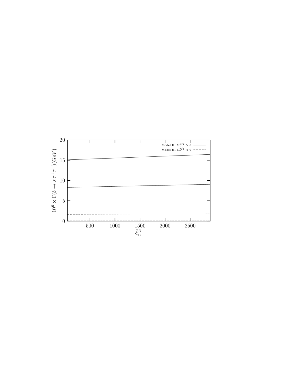
Figure 12: The same as Fig. 11 for $\bar{\xi}_{N,bb}^{D}=0.1\,m_{b}$ in case of the ratio $r_{tb}>1$.

Figure 13: Differential $A_{FB}$ as a function of $s$ for $\bar{\xi}_{N,bb}^{D}=40\,m_{b}$, $\bar{\xi}_{N,\tau\tau}^{D}=1\,GeV$ and $m_{H^{\pm}}=400\,GeV$ including LD effects in case of the ratio $|r_{tb}|<1$.

Figure 14: $A_{FB}$ as a function of $\frac{\bar{\xi}_{N,bb}^{D}}{m_{b}}$ for $\bar{\xi}_{N,\tau\tau}^{D}=1\,GeV$, $m_{H^{\pm}}=400\,GeV$ and $|r_{tb}|<1$.

Figure 15: The same as Fig. 14 but for $r_{tb}>1$.

References

[1] J. L. Hewett, in Proc. of the Annual SLAC Summer
Institute, ed. L. De Porcel and C. Dunwoode, SLAC-PUB-6521 (1994)
[2] W. -S. Hou, R. S. Willey and A. Soni,
Phys. Rev. Lett.58 (1987) 1608.
[3] N. G. Deshpande and J. Trampetic,
Phys. Rev. Lett.60 (1988) 2583.
[4] C. S. Lim, T. Morozumi and A. I. Sanda,
Phys. Lett.B218 (1989) 343.
[5] B. Grinstein, M. J. Savage and M. B. Wise,
Nucl. Phys.B319 (1989) 271.
[6] C. Dominguez, N. Paver and Riazuddin,
Phys. Lett.B214 (1988) 459.
[7] N. G. Deshpande, J. Trampetic and K. Ponose,
Phys. Rev.D39 (1989) 1461.
[8] P. J. O’Donnell and H. K. Tung,
Phys. Rev.D43 (1991) 2067.
[9] N. Paver and Riazuddin,
Phys. Rev.D45 (1992) 978.
[10] A. Ali, T. Mannel and T. Morozumi,
Phys. Lett.B273 (1991) 505.
[11] A. Ali, G. F. Giudice and T. Mannel,
Z. Phys.C67 (1995) 417.
[12] C. Greub, A. Ioannissian and D. Wyler,
Phys. Lett.B346 (1995) 145;
D. Liu Phys. Lett.B346 (1995) 355;
G. Burdman, Phys. Rev.D52 (1995) 6400:
Y. Okada, Y. Shimizu and M. Tanaka Phys. Lett.B405 (1997) 297.
[13] A. J. Buras and M. Münz,
Phys. Rev.D52 (1995) 186.
[14] N. G. Deshpande, X. -G. He and J. Trampetic,
Phys. Lett.B367 (1996) 362.
[15] W. Jaus and D. Wyler,
Phys. Rev.D41 (1990) 3405.
[16] Y. B. Dai, C.S. Huang and H. W. Huang
Phys. Lett.B390 (1997) 257,
C. S. Huang, L. Wei, Q. S. Yan
and S. H. Zhu, hep-ph/0006250.
[17] H. E. Logan and U. Nierste, Nucl. Phys.B586
(2000) 39.
[18] D. Atwood, L. Reina and A. Soni,
Phys. Rev.D55 (1997) 3156.
[19] T. M. Aliev, and E. Iltan,
Phys. Rev.D58 (1998) 095014.
[20] M. S. Alam, CLEO Collaboration, to appear in ICHEP98
Conference (1998)
[21] T. M. Aliev, and E. Iltan, J. Phys. G25 (1999) 989.
[22] B. Grinstein, R. Springer, and M. Wise,
Nucl. Phys. B339 (1990) 269; R. Grigjanis, P.J. O’Donnel,
M. Sutherland and H. Navelet, Phys. Lett. B213 (1988) 355;
Phys. Lett. B286 (1992) E, 413;
G. Cella, G. Curci, G. Ricciardi and
A. Viceré, Phys. Lett. B325 (1994) 227,
Nucl. Phys. B431 (1994) 417.