The rare decay $\boldsymbol{b\rightarrow sg}$ beyond leading logarithms

Abstract

We calculate the $O(\alpha_{s})$ virtual corrections to the decay width for $b\rightarrow sg$ in the standard model ($g$ denotes a gluon). Also the corresponding $O(\alpha_{s})$ bremsstrahlung corrections to $b\rightarrow sg$ are systematically calculated in this paper. The combined result is free of infrared and collinear singularities, in accordance with the KLN theorem. Taking into account the existing next-to-leading logarithmic (NLL) result for the Wilson coefficient $C_{8}^{\rm{eff}}$, a complete NLL result for the branching ratio ${\cal B}^{\rm{NLL}}(b\rightarrow sg)$ is derived. Numerically, we obtain ${\cal B}^{\rm{NLL}}=(5.0\pm 1.0)\times 10^{-3}$, which is more than a factor of two larger than the leading logarithmic result ${\cal B}^{\rm{LL}}=(2.2\pm 0.8)\times 10^{-3}$.

I Introduction

The theoretical predictions for inclusive decay rates of $B$-mesons rest on solid gounds due to the fact that these rates can be sytematically expanded in powers of $(\Lambda_{\rm QCD}/m_{b})$ [1, 2], where the leading term corresponds to the decay width of the underlying $b$-quark decay. As the power corrections start at $O(\Lambda_{\rm{QCD}}/m_{b})^{2}$ only, they affect these rates by at most 5%. Thus the accuracy of the theoretical predictions is mainly controlled by our knowledge of the perturbative corrections to the free quark decay.

The charmless inclusive decays, $B\rightarrow X_{c/}$, where $X_{c/}$ denotes any hadronic charmless final state, are an interesting subclass of the decays mentioned above. At the quark level, there are decay modes with three-body final states, viz. $b\rightarrow q^{\prime}\overline{q}^{\prime}q$, ($q^{\prime}=u,d,s$; $q=d,s$) and the modes $b\rightarrow qg$, with two-body final state topology, which contribute to the charmless decay width at leading logarithmic (LL) accuracy. Next-to-leading logarithmic (NLL) corrections to the three-body decay modes were started already some time ago in ref. [3], where radiative corrections to the current-current diagrams of the operators $O_{1}$ and $O_{2}$ were calculated, together with NLL corrections to the Wilson coefficients. Later, Lenz et al. [4, 5] included the contributions of the penguin diagrams associated with the four-Fermi operators $O_{1},...,O_{6}$; the effects of the chromomagnetic operator $O_{8}$ were taken into account to the relevant precision needed for a NLL calculation. Up to contributions from current-current type corrections to the penguin operators, the NLL calculation for the three quark final states is complete.

In the numerical evaluations of the charmless decay rate, the two body decay modes $b\rightarrow qg$ were added in refs. [4, 5] at the LL precision, as the full NLL predictions were missing. It is exactly this gap which we try to fill in the present letter. We will present the results of a calculation for the branching ratio ${\cal B}(b\rightarrow sg)$ where NLL corrections are systematically included. This implies that besides virtual corrections to $b\rightarrow sg$ also the process $b\rightarrow sgg$ has to be taken into account, as it gives contributions at the same order in perturbation theory. The LL prediction for the branching for $b\rightarrow sg$ is known to be ${\cal B}(b\rightarrow sg)\approx 0.2\%$ [6]; also the process $b\rightarrow sgg$ has been studied in the literature [7, 8]. In [8] a complete calculation was performed in regions of the phase space which are free of collinear an infrared singularities, leading to a branching ratio for $b\rightarrow sgg$ of the order of $10^{-3}$. A complete NLL calculation requires, however, a regularized version for the decay width $\Gamma(b\rightarrow sgg)$ in which infrared and collinear singularities become manifest. Only after adding the virtually corrected decay width $\Gamma(b\rightarrow sg)$ a meaningful physical result is obtained. In addition, as we will see later, also the tree-level contribution of the operator $O_{8}$ to the decays $b\rightarrow sf\overline{f}$, with $f=u,d,s$, has to be included.

The decay $b\rightarrow sg$ gained a lot of attention in the last years. For a long time the theoretical predictions for both, the inclusive semileptonic branching ratio and the charm multiplicity $n_{c}$ in $B$-meson decays were considerably higher than the experimental values [9]. An attractive hypothesis, which would move the theoretical predicitions for both observables into the direction favored by the experiments, assumed the rare decay mode $b\rightarrow sg$ to be enhanced by new physics.

After the inclusion of the complete NLL corrections to the decay modes $b\rightarrow c\overline{u}q$ and $b\rightarrow c\overline{c}q$ ($q=d,s$) [10], both the CLEO- and the LEP-data [11] are now in agreement with theory [10, 12], if one allows the renormalization scale $\mu$ to become as low as $m_{b}/4$. We would like to stress that there is still some room for enhanced $b\rightarrow sg$, in particular when using higher values for the renormalization scale. For theoretical motivations of enhanced $b\rightarrow sg$, see ref. [13] and references therein.

We also would like to mention that the component $b\rightarrow sg$ of the charmless hadronic decays is expected to manifest itself in kaons with high momenta (of order $m_{b}/2$), due to its two body nature [14]. Some indications into this direction were reported by the SLD collaboration [15]. For overviews on enhanced $b\rightarrow sg$, see e.g. refs. [16, 17].

The remainder of this letter is organized as follows: In section II, we briefly review the theoretical framework. Section III is devoted to the calculation of the virtual corrections to the decay width for $b\rightarrow sg$, while section V deals with the calculation of the bremsstrahlung corrections to $b\rightarrow sg$. In the short section IV in between, the decay width for the tree level processes $b\rightarrow sf\overline{f}$ mentioned above, is given. In section VI we give the expressions for the NLL branching ratio ${\cal B}^{\rm{NLL}}(b\rightarrow sg)$, which combines the processes $b\rightarrow sg$, $b\rightarrow sgg$ and $b\rightarrow sf\overline{f}$. Finally, in section VII the numerical results for ${\cal B}^{\rm{NLL}}(b\rightarrow sg)$ are presented.

II Theoretical framework

The analysis of the decays $b\rightarrow sg$ and $b\rightarrow sgg$ starts with introducing the effective Hamiltonian

$${\cal H}_{\rm eff}=-\frac{4G_{F}}{\sqrt{2}}\,V_{ts}^{*}V_{tb}\sum_{i=1}^{8}C_{i}(\mu)O_{i}(\mu).$$ (1)

where $V_{ij}$ are elements of the CKM matrix, $O_{i}(\mu)$ are the relevent operators and $C_{i}(\mu)$ are the corresponding Wilson coefficients. The full set of operators needed for our application, can be seen in ref. [18]. As the Wilson coefficients of the gluonic penguin operators are small (see eq. (30) in ref. [18]), we neglect them when calculating radiative corrections; we therefore only list the explicit form of the operators $O_{1}$, $O_{2}$ and $O_{8}$:

$$\begin{array}[]{llll}O_{1}\,=&\!(\overline{s}_{L}\gamma_{\mu}T^{A}c_{L})\,(\overline{c}_{L}\gamma^{\mu}T^{A}b_{L})\,,&\quad O_{2}\,=&\!(\overline{s}_{L}\gamma_{\mu}c_{L})\,(\overline{c}_{L}\gamma^{\mu}b_{L})\,,\\[4.31415pt] O_{8}\,=&\!\frac{g_{s}}{16\pi^{2}}\,{\overline{m}}_{b}(\mu)\,(\overline{s}_{L}\sigma^{\mu\nu}T^{A}b_{R})\,G^{A}_{\mu\nu}\ .\end{array}$$ (2)

Here $T^{A}$ stand for the $SU(3)_{\rm{color}}$ generators. The small CKM matrix element $V_{ub}$ as well as the $s$-quark mass are also neglected.

It is well-known that in this formalism the large QCD logarithms, present in the decay amplitude for $b\rightarrow sg$, are contained in resummed form in the Wilson coefficients when choosing the renormalization scale $\mu$ at the order of $m_{b}$. The LL (NLL) Wilson coefficients contain all terms of the form $\alpha_{s}^{n}\ln^{n}(m_{b}/M)$ $(\alpha_{s}\,\alpha_{s}^{n}\ln^{n}(m_{b}/M))$, where $M=m_{t}$ or $m_{W}$ and $n=0,1,2,\ldots$.

The LL prediction for the decay amplitude for $b\rightarrow sg$ is then obtained by calculating the matrix elements $\langle sg|O_{i}|b\rangle$ at order $g_{s}$ and weighting them with the leading logarithmic Wilson coefficients. In the naive dimensional regularization (NDR) scheme which we use in this paper, there are one-loop contributions of order $g_{s}$ for $i=3,4,5,6$ and the tree-level contribution of $O_{8}$. The effect of the matrix elements for $i=3,4,5,6$ can be absorbed into the effective Wilson coefficient (see [18]) $C_{8}^{\rm{eff}}=C_{8}+C_{3}-{\textstyle\frac{1}{6}}\,C_{4}+20\,C_{5}-{\textstyle\frac{10}{3}}\,C_{6}$.

The NLL corrections for the decay amplitude for $b\rightarrow sg$ receives two contributions: The first one arises when combining the lowest order matrix elements (of order $g_{s}$) with the NLL Wilson coefficient, while the second one arises when calculating explicit order $\alpha_{s}$ corrections to the matrix elements of the operators which are then weighted with LL Wilson coefficients. As the operators $O_{1}$ and $O_{2}$ have vanishing matrix elements for $b\rightarrow sg$ at order $g_{s}$ and the NLL corrections connected with the operators $O_{3},...,O_{6}$ are neglected, the only Wilson coefficient needed to NLL precision is that of the operator $O_{8}$. The necessary ingredients, the anomalous dimension matrix to $O(\alpha_{s}^{2})$ and the $O(\alpha_{s})$ matching condition for the operator $O_{8}$ were given in refs. [18] and [19], respectively. A practical parametrization for $C_{8}^{\rm{eff}}(\mu)$ will be given in ref. [20]. A rather complete list of references on matching conditions, anomalous dimension matrices, and on the process $b\rightarrow s\gamma$, which is similar in many respects to $b\rightarrow sg$, is given e.g. in ref. [21].

III Virtual corrections to $\boldsymbol{O_{1}}$, $\boldsymbol{O_{2}}$ and $\boldsymbol{O_{8}}$

A Virtual corrections to $\boldsymbol{O_{1}}$ and $\boldsymbol{O_{2}}$

As the one-loop matrix elements of the operators $O_{1}$ and $O_{2}$ vanish, we immediately turn to the two-loop contributions. A complete list of Feynman diagrams for the matrix elements $\langle sg|O_{i}|b\rangle$ ($i=1,2$) is shown in fig. 1.

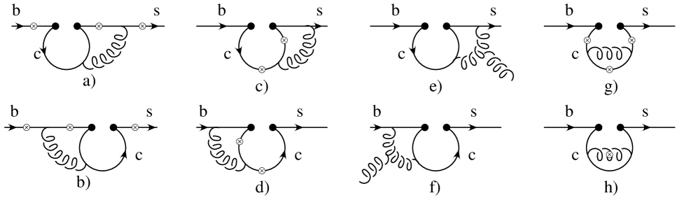
FIG. 1.: Complete List of two-loop Feynman diagrams for $b\rightarrow sg$ associated with the operators $O_{1}$ and $O_{2}$. The fermions ($b$, $s$ and $c$ quarks) are represented by solid lines; the wavy lines represent gluons. The crosses denote the possible locations where the gluon is emitted.

The diagrams in fig. 1 a), b), c) and d), in which the emitted gluon is replaced by a photon are the relevant diagrams for $b\rightarrow s\gamma$; these were calculated in ref. [22]. The three possible diagrams in fig. 1 g) cancel each other when considering the process $b\rightarrow s\gamma$; however, they give a non-vanishing contribution to $b\rightarrow sg$. There is also another difference: while each of the figures a), b), c) and d) forms a gauge invariant subset in $b\rightarrow s\gamma$, this is no longer true for $b\rightarrow sg$; a gauge invariant result is only obtained when all the diagrams in fig. 1 are summed.

The various two-loop integrals are calculated by the standard Feynman parameter technique. The heart of our procedure, which is explained in detail in ref. [22] for one of the diagrams in fig. 1 a), is to represent the rather complicated denominators in the Feynman parameter integrals as complex Mellin-Barnes integrals [23]. After inserting this representation and interchanging the order of integration, the Feynman parameter integrals are reduced to well-known Euler Beta-functions. Finally, the residue theorem allows to represent the remaining complex integal as the sum over the residues taken at the pole positions of Beta- and Gamma-functions; for a generic diagram $G$, these steps naturally lead to an expansion in the ratio $z=(m_{c}/m_{b})^{2}$ of the form

$$G=c_{0}+\sum_{n,m}c_{nm}z^{n}L^{m}\quad;\quad z=\frac{m_{c}^{2}}{m_{b}^{2}}\quad;\quad L=\ln z\ ,$$ (3)

where the coefficients $c_{0}$ and $c_{nm}$ are independent of $z$. The power $n$ in eq. (3) is in general a natural multiple of $1/2$ and $m$ is a natural number including 0. In the explicit calculation, the lowest $n$ turns out to be $n=1$. This implies the important fact that the limit $m_{c}\rightarrow 0$ exists. As was shown in [22], the power $m$ of the logarithm is bounded by $4$, independently of the value of $n$. In our results, which we will present below, all terms up to $n=3$ are retained.

We first present the final result for the dimensionally regularized matrix element $M_{2}=\langle sg|O_{2}|b\rangle$ which represents the sum of all two-loop diagrams in fig. 1:

$$M_{2}=\frac{\alpha_{s}}{4\pi}\langle sg|O_{8}|b\rangle_{\text{tree}}\left[-\frac{16}{27\,\epsilon}\left(\frac{m_{b}}{\mu}\right)^{-4\epsilon}+r_{2}\,\right]\ ,$$ (4)

where the real- and imaginary part of $r_{2}$ read

$$\mbox{Re}(r_{2}) = \frac{1}{648}\big{\{}-2170-54\pi^{2}+z[48816-252\pi^{2}+(22680-1620\pi^{2})L$$ (9)

$$\quad+2808L^{2}+612L^{3}-6480\zeta(3)]$$

$$\quad-12672\pi^{2}z^{3/2}+z^{2}[66339+1872\pi^{2}+(-40446+1512\pi^{2})L$$

$$\quad+6642L^{2}-1008L^{3}+7776\zeta(3)]$$

$$\quad+z^{3}[-3420-60\pi^{2}-6456L+7884L^{2}]\big{\}}$$

$$\mbox{Im}(r_{2}) = \frac{\pi}{27}\big{\{}-28+z[549-24\pi^{2}+153L+72L^{2}]$$ (11)

$$\quad+z^{2}[-432+30\pi^{2}+54L-90L^{2}]+z^{3}[-259+192L]\big{\}}\ .$$

The symbol $\zeta$ stands for the Riemann Zeta function, with $\zeta(3)\approx 1.2021$. Finally, the quantity $\langle sg|O_{8}|b\rangle_{\text{tree}}$ denotes the tree level matrix element of the operator $O_{8}$.

To obtain the renormalized matrix element $M_{2}^{\rm{ren}}$ associated with the operator $O_{2}$, the corresponding counterterms have to be included. This means that we have to take into account the one-loop matrix elements of the four Fermi operators $\delta Z_{2j}O_{j}$ ($j=1,...,6$) and the tree level contribution of the magnetic operator $\delta Z_{28}O_{8}$. In the NDR scheme the only non-vanishing contributions to $b\rightarrow sg$ come from $j=4,8$. The operator renormalization constants $Z_{ij}$ can be extracted from the literature [18] in the context of the leading order anomalous dimension matrix. One obtains the counterterm contribution

$$M_{2}^{\rm{ct}}=\langle sg|\delta Z_{24}O_{4}+\delta Z_{28}O_{8}|b\rangle=\left(-\frac{\alpha_{s}}{36\pi}\,\frac{1}{\epsilon}\left(\frac{m_{b}}{\mu}\right)^{-2\epsilon}+\frac{\alpha_{s}}{\pi}\,\frac{19}{108}\,\frac{1}{\epsilon}\right)\langle sg|O_{8}|b\rangle_{\text{tree}}\quad.$$ (12)

We note that there are no one-loop contributions to the matrix element for $b\rightarrow sg$ from counterterms proportional to the evancesent operator $P_{12}$ given in appendix A of ref. [18]. Adding the regularized two-loop result in eq. (4) and the counterterm in eq. (12), we find the renormalized result for $M_{2}$ in the NDR scheme:

$$M_{2}^{\rm{ren}}=\langle sg|O_{8}|b\rangle_{\text{tree}}\,\frac{\alpha_{s}}{4\pi}\,\left(\ell_{2}\ln\frac{m_{b}}{\mu}+r_{2}\right)\quad,$$ (13)

where $r_{2}$ is given in eq. (9) and $\ell_{2}=70/27$.

By doing analogous steps, we obtain the renormalized version of $M_{1}=\langle sg|O_{1}|b\rangle$:

$$M_{1}^{\rm{ren}}=\langle sg|O_{8}|b\rangle_{\text{tree}}\,\frac{\alpha_{s}}{4\pi}\,\left(\ell_{1}\ln\frac{m_{b}}{\mu}+r_{1}\right)\quad,$$ (14)

with $\ell_{1}=173/162$ and

$$\mbox{Re}(r_{1}) = -\frac{1}{3888}\big{\{}4877-54\pi^{2}+36z[1086+29\pi^{2}+(360+36\pi^{2})L$$ (19)

$$\quad+51L^{2}+8L^{3}+144\zeta(3)]$$

$$\quad-12672\pi^{2}z^{3/2}+9z^{2}[6615-80\pi^{2}+(-4494+384\pi^{2})L$$

$$\quad+864L^{2}-148L^{3}+864\zeta(3)]$$

$$\quad+12z^{3}[93+76\pi^{2}-1186L+900L^{2}]\big{\}}$$

$$\mbox{Im}(r_{1}) = -\frac{\pi}{324}\big{\{}25+6z[75+\pi^{2}+24L-3L^{2}]$$ (21)

$$\quad+6z^{2}[-171+19\pi^{2}+72L-57L^{2}]+2z^{3}[-421+192L]\big{\}}$$

For $z\geq 1/4$ the imaginary parts of $r_{1}$ and $r_{2}$ must vanish exactly; our results fulfill this property to high accuracy when retaining terms up to $z^{3}$ in the expansion.

B Virtual corrections to $\boldsymbol{O_{8}}$

We present now the results of the virtual corrections to the matrix element $M_{8}=\langle sg|O_{8}|b\rangle$.

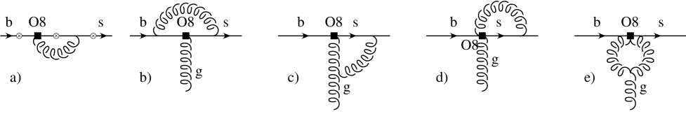
FIG. 2.: Complete list of Feynman diagrams associated with the operator $O_{8}$. The analogues of a), c) and d), where the virtual gluon hits the $b$-quark instead of the $s$-quark, are not shown explicitly. The real gluon can be attached to any of the crosses shown in a).

As the contributing Feynman graphs in fig. 2 are all one loop diagrams, the computation of $M_{8}$ is straightforward. We use dimensional regularization for both, the ultraviolet and the infrared singularities. Singularities which appear in the situation where the virtual gluon becomes almost real and collinear with the emitted gluon are also regulated dimensionally; on the other hand, those singularities where the almost real internal gluon is collinear with the $s$-quark, are regulated with a small strange quark mass $m_{s}$; the latter manifest themselves in logarithmic terms of the form $\ln(\rho)$, where $\rho=(m_{s}/m_{b})^{2}$.

We were able to separate the ultraviolet $1/\epsilon$ poles from those which are of infrared (and/or collinear) origin. For ultraviolet poles we use the symbol $1/\epsilon$ in the following, while collinear and infrared poles are denoted by $1/\epsilon_{\rm IR}$.

As the results of the individual diagrams are not very instructive, we only give their sum:

$$M_{8}=\frac{\alpha_{s}}{4\pi}\,f_{8}\,\langle sg|O_{8}|b\rangle_{\text{tree}}\ ,$$ (22)

with

$$f_{8} = \left[\,-\frac{3}{\epsilon_{\rm IR}^{2}}-\frac{(4\ln(\rho)+9+9i\pi)}{3\epsilon_{\rm IR}}+\frac{11}{3\epsilon}\right]\,\left(\frac{m_{b}}{\mu}\right)^{-2\epsilon}+$$ (24)

$$\quad\frac{1}{3}\,\left[\frac{59\pi^{2}}{12}+1-8\ln(\rho)+2\ln^{2}(\rho)-8i\pi\right]\ .$$

An ultraviolet finite result is obtained by adding the contribution from the counterterm which is generated by expressing the bare quantities in the tree-level matrix element of $O_{8}$ by their renormalized counterparts. It has the structure

$$M_{8}^{\rm{ct}}=\delta R\,\langle sg|O_{8}|b\rangle_{\text{tree}}\quad,$$ (25)

where the factor $\delta R$ is given by $\delta R=\sqrt{Z_{2}(m_{b})}\,\sqrt{Z_{2}(m_{s})}\,\sqrt{Z_{3}}\,Z_{g_{s}}\,Z_{m_{b}}\,Z_{88}\,-\,1\$.

$Z_{2}(m_{b})$, $Z_{2}(m_{s})$ and $Z_{3}$ denote the on-shell wave function renormalization factors of the $b$-quark, the $s$-quark and the gluon, respectively. $Z_{g_{s}}$ and $Z_{m_{b}}$ denote the $\overline{\mbox{MS}}$ renormalization constants for the strong coupling constant $g_{s}$ and the $b$-quark mass, which appear explicitly in the definition of the operators (see eq. (2)). Finally, $Z_{88}$ is the renormalization factor of the operator $O_{8}$. The $Z$-factors of the fields, of the masses and of the strong coupling constant are given in text books, while $Z_{88}$ can be extracted from the anomalous dimension matrix in ref. [18]; we therefore immediately give the expression for $\delta R$:

$$\ \delta R=-\frac{\alpha_{s}}{4\pi}\,\left[\frac{11}{3\epsilon}+\frac{31}{6\epsilon_{\rm IR}}-8\ln\frac{m_{b}}{\mu}-\frac{2}{3}\sum_{f}\ln\frac{m_{f}}{\mu}+\frac{16}{3}-2\ln\rho\right]\ .$$ (26)

The term $\sum_{f}$ originates from fermion self-energy diagrams contributing to the on-shell renormalization constant $Z_{3}$ of the gluon field; $f$ runs over the five flavors $u$, $d$, $s$, $c$ and $b$.

When adding the regularized matrix element of $O_{8}$ in eq. (22) and the counterterm contribution $M_{8}^{\rm{ct}}$ in eq. (25), we obtain the renormalized result

$$M_{8}^{\rm{ren}}=\frac{\alpha_{s}}{4\pi}\,f_{8}^{\rm{ren}}\,\langle sg|O_{8}|b\rangle_{\text{tree}}\ ,$$ (27)

with

$$f_{8}^{\rm{ren}} = \left[\,-\frac{3}{\epsilon_{\rm IR}^{2}}-\frac{(8\ln(\rho)+49+18i\pi)}{6\epsilon_{\rm IR}}\right]\,\left(\frac{m_{b}}{\mu}\right)^{-2\epsilon}-\frac{29}{3}\ln\frac{m_{b}}{\mu}$$ (29)

$$\quad+\frac{2}{3}\sum_{f}\ln\frac{m_{f}}{\mu}\,-5+\frac{59\pi^{2}}{36}-\frac{2}{3}\ln\rho+\frac{2}{3}\ln^{2}\rho-\frac{8}{3}i\pi\ .$$

We anticipate that the singular terms of the form $1/\epsilon^{2}_{\rm IR}$, $1/\epsilon_{\rm IR}$ and $\ln\rho$ in eq. (29) will cancel against the corresponding singularities in the result for the gluon bremsstrahlung corrections to $b\rightarrow sg$. On the other hand, the terms $\ln(m_{f}/\mu)$, which also represent some kind of singularities for the light flavor $f=u,d,s$ are not cancelled in this way. Keeping in mind that they originate from the fermionic contribution to the renormalization factor $Z_{3}$, it is expected that they will cancel against the logarithms present in the decay rate $\Gamma(b\rightarrow sf\overline{f})$ ($f=u,d,s$).

C Virtual corrections to the decay width $\boldsymbol{\Gamma(\char 98\relax\rightarrow\char 115\relax\char 103\relax})$

We are now in the position to write down the renormalized version of the matrix $M^{\rm{ren}}(b\rightarrow sg)$ element for $b\rightarrow sg$, where the virtual order $\alpha_{s}$ corrections are included. We obtain:

$$M^{\rm{ren}}(b\rightarrow sg) = \frac{4G_{F}i}{\sqrt{2}}\,V_{ts}^{*}V_{tb}\,\bigg{\{}C_{8}^{\rm{eff}}+\frac{\alpha_{s}}{4\pi}\bigg{[}C_{1}^{0}(\ell_{1}\ln\frac{m_{b}}{\mu}+r_{1})+C_{2}^{0}(\ell_{2}\ln\frac{m_{b}}{\mu}+r_{2})+$$ (31)

$$\quad C_{8}^{0,\rm{eff}}\,f_{8}^{\rm{ren}}\,\bigg{]}\bigg{\}}\,\langle sg|O_{8}(\mu)|b\rangle_{\rm{tree}}.$$

The quantities $r_{1}$, $r_{2}$ and $f_{8}^{\rm{ren}}$ are given in eqs. (19), (9) and (29), respectively. As eq. (31) shows, $C_{8}^{\rm eff}$ is the only Wilson coefficient needed to NLL precision. For the following it is useful to decompose it as

$$C_{8}^{\rm{eff}}=C_{8}^{0,\rm{eff}}+\frac{\alpha_{s}}{4\pi}\,C_{8}^{1,\rm{eff}}\ .$$ (32)

The symbol $\langle sg|O_{8}(\mu)|b\rangle_{\rm{tree}}$ in eq. (31) denotes the tree level matrix element of $O_{8}(\mu)$, which contains the running $b$-quark mass and the strong running coupling constant at the scale $\mu$. In order to get expressions where the $b$-quark mass enters as the pole mass, and the strong coupling constant enters as $g_{s}(m_{b})$, we rewrite $\langle sg|O_{8}(\mu)|b\rangle_{\rm{tree}}$ as

$$\langle sg|O_{8}(\mu)|b\rangle_{\rm{tree}}=\langle sg|O_{8}|b\rangle_{\rm{tree}}\,\left[1+\frac{2\alpha_{s}}{\pi}\ln\frac{m_{b}}{\mu}-\frac{4}{3}\frac{\alpha_{s}}{\pi}+\frac{\alpha_{s}}{4\pi}\,\beta_{0}\,\ln\frac{m_{b}}{\mu}\right]\ ;\quad\beta_{0}=\frac{23}{3}\ .$$ (33)

The symbol $\langle sg|O_{8}|b\rangle_{\rm{tree}}$ then stands for the tree level matrix element of $O_{8}$ in which $\overline{m}_{b}(\mu)$ and $g_{s}$ have to to be indentified with the pole mass $m_{b}$ and $g_{s}(m_{b})$, respectively. After inserting eqs. (32) and (33) into eq. (31), the corresponding decay width $\Gamma^{\rm{virt}}$ is obtained in the standard way. One gets:

$$\Gamma^{\rm{virt}} = \frac{\alpha_{s}(m_{b})\,m_{b}^{5}}{24\pi^{4}}|G_{F}V_{ts}^{*}V_{tb}|^{2}\,\left\{\left(C_{8}^{0,\rm{eff}}\right)^{2}+\frac{\alpha_{s}}{4\pi}\,C_{8}^{0,\rm{eff}}\,\left[2\,C_{8}^{1,\rm{eff}}+2(8+\beta_{0})\ln\frac{m_{b}}{\mu}\,C_{8}^{0,\rm{eff}}\right.\right.$$ (36)

$$-\frac{32}{3}C_{8}^{0,\rm{eff}}+2\,C_{1}^{0}(\ell_{1}\,\ln\frac{m_{b}}{\mu}+\mbox{Re}(r_{1}))+2\,C_{2}^{0}(\ell_{2}\,\ln\frac{m_{b}}{\mu}+\mbox{Re}(r_{2}))$$

$$\left.\left.\quad+2\,C_{8}^{0,\rm{eff}}\mbox{Re}(f_{8}^{\rm{ren}})\,(1-\epsilon)\,\left(\frac{m_{b}}{\mu}\right)^{-2\epsilon}\,\left(1+2\epsilon-\frac{1}{4}(\pi^{2}-16)\epsilon^{2}\right)\right]\right\}\ .$$

We note that due to the infrared poles present in $f_{8}^{\rm{ren}}$ the phase space integrations were done consistently in $d=4-2\epsilon$ dimensions.

IV $\boldsymbol{O_{8}}$ contribution to the decay width $\boldsymbol{\Gamma(\char 98\relax\rightarrow\char 115\relax\char 102\relax\bar{\char 102\relax}})$

As discussed at the end of section III B, we should take into account the contribution of the operator $O_{8}$ to the process $b\rightarrow sf\overline{f}$ $(f=u,d,s)$, in order to cancel the unphysical logarithms of the form $\ln(m_{f}/\mu)$ in the virtual corrections to $b\rightarrow sg$. The $O_{8}$ contribution to the decay width $\Gamma_{8}(b\rightarrow sf\overline{f})$ yields

$$\Gamma_{8}(b\rightarrow sf\overline{f})=\frac{m_{b}^{5}\,|G_{F}\,V_{ts}^{*}V_{tb}\,C_{8}^{0,\rm{eff}}|^{2}}{72\pi^{5}}\,\alpha_{s}^{2}\,\left[\ln\frac{m_{b}}{2m_{f}}-\frac{2}{3}\right]\ .$$ (37)

V Gluon bremsstrahlung contributions

In this section we discuss the gluon bremsstrahlung corrections to $b\rightarrow sg$, i.e. the process $b\rightarrow sgg$. As in the case of the virtual corrections, we neglect contributions from the gluonic penguin operators as their Wilson coefficients are rather small. In this approximation, the matrix element $M^{\rm{brems}}(b\rightarrow sgg)$ is of the form

$$M^{\rm{brems}}=\frac{4G_{F}i}{\sqrt{2}}\,V_{ts}^{*}V_{tb}\,\left[C_{1}^{0}\,M_{1}^{\rm{brems}}+C_{2}^{0}\,M_{2}^{\rm{brems}}+C_{8}^{0,\rm{eff}}\,M_{8}^{\rm{brems}}\right]\ ,$$ (38)

where the three terms on the r.h.s. correspond to the contributions of the operators $O_{1}$, $O_{2}$ and $O_{8}$, respectively. The corresponding Feynman diagrams are shown in fig. 3. We note that in eq. (38) only the leading order pieces of the Wilson coefficients are needed.

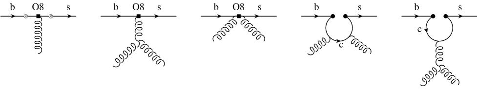
FIG. 3.: Complete list of Feynman diagrams for $b\rightarrow sgg$, associated with the operators $O_{1}$, $O_{2}$ and $O_{8}$.

The decay width $\Gamma^{\rm{brems}}(b\rightarrow sgg)$ is then obtained by squaring $M^{\rm{brems}}$, followed by phase space integrations. These integrals are plagued with infrared and collinear singularities. Configurations with one gluon flying collinear to the $s$-quark are regulated by a small strange quark mass $m_{s}$, while configurations with two collinear gluons, or one soft gluon are dimensionally regularized. As in the calculations of the virtual corrections, we write the dimension as $d=4-2\epsilon$. (Note that $\epsilon$ has to be negative in order to regulate the phase space integrals).

When squaring $M^{\rm{brems}}$ in eq. (38), nine terms are generated, which we denote for obvious reasons by $(O_{1},O_{1}^{*})$, $(O_{1},O_{2}^{*})$, $(O_{1},O_{8}^{*})$, $(O_{2},O_{1}^{*})$, …., $(O_{8},O_{8}^{*})$. We find that all these quantities are free of infrared and collinear singularities, except $(O_{8},O_{8}^{*})$. Hence, one can put $m_{s}=0$ in the finite terms and evaluate the phase space integrals in $d=4$ dimensions. In the following, we denote this finite contribution to the decay width by $\Gamma^{\rm{brems}}_{\rm{fin}}$. It turns out that only $\sim 5\%$ of the total NLL correction are due to $\Gamma^{\rm{brems}}_{\rm{fin}}$. As the analytical results for this finite piece, written in terms of two-dimensional integrals, are rather lengthy, we skip the explicit expressions in this letter; we stress, however, that $\Gamma^{\rm{brems}}_{\rm{fin}}$, although small, will be retained in the numerical evaluations.

We now turn to the $(O_{8},O_{8}^{*})$ contribution, denoted by $\Gamma^{\rm{brems}}_{88}$. After a lengthy, but straightforward calculation, we obtain ($\rho=(m_{s}/m_{b})^{2}$; $V=\alpha_{s}\,m_{b}^{5}\,|G_{F}V_{ts}^{*}V_{tb}|^{2}/(24\pi^{4})$)

$$\Gamma^{\rm{brems}}_{\rm{88}}=\frac{\alpha_{s}\left(C_{8}^{0,\rm{eff}}\right)^{2}\,V\,\left(\frac{m_{b}}{\mu}\right)^{-4\epsilon}}{12\,\pi}\,\,\left[\frac{18}{\epsilon^{2}_{\rm{IR}}}+\frac{67+8\ln\rho}{\epsilon_{\rm IR}}-4\ln^{2}\rho+12\ln\rho+240-\frac{62\pi^{2}}{3}\right]\ .$$ (39)

The total decay with for $b\rightarrow sgg$ is then given by

$$\Gamma^{\rm{brems}}(b\rightarrow sgg)=\Gamma^{\rm{brems}}_{\rm{fin}}+\Gamma^{\rm{brems}}_{88}\ .$$ (40)

VI Combined NLL branching ratio for $\boldsymbol{\char 98\relax\rightarrow\char 115\relax\char 103\relax}$ and $\boldsymbol{\char 98\relax\rightarrow\char 115\relax\char 103\relax\char 103\relax}$

In this section we combine the decay widths for the virtually corrected process $b\rightarrow sg$ and the bremsstrahlung process $b\rightarrow sgg$ to the total NLL decay width decay $\Gamma^{\rm{NLL}}(b\rightarrow sg)$. We also absorbe in this quantity the $O_{8}$ induced contribution to the processes $b\rightarrow sf\overline{f}$ ($f=u,d,s$), as discussed in section IV. From the explicit formulas for $\Gamma^{\rm{virt}}$ and $\Gamma^{\rm{brems}}$ one can see that the infrared and collinear singularities cancel in the sum. The terms containing logarithms of the light quark masses $m_{f}$, present in the result for $\Gamma^{\rm{virt}}$, are cancelled when combined with $\Gamma_{8}(b\rightarrow sf\overline{f})$. Putting together the individual pieces, the final result for $\Gamma^{\rm{NLL}}(b\rightarrow sg)$ can be written as

$$\Gamma^{\rm{NLL}}(b\rightarrow sg)=\frac{\alpha_{s}(m_{b})\,m_{b}^{5}}{24\pi^{4}}|G_{F}V_{ts}^{*}V_{tb}|^{2}\,|\overline{D}|^{2}+\Gamma_{\rm{fin}}^{\rm{brems}}\ ,$$ (41)

with

$$\overline{D} = C_{8}^{0,\rm{eff}}+\frac{\alpha_{s}}{4\pi}\,\left[C_{8}^{1,\rm{eff}}-\frac{16}{3}C_{8}^{0,\rm{eff}}+C_{1}^{0}[\ell_{1}\,\log\frac{m_{b}}{\mu}+r_{1}]\right.$$ (43)

$$\left.\quad\quad\quad+C_{2}^{0}[\ell_{2}\,\log\frac{m_{b}}{\mu}+r_{2}]+C_{8}^{0,\rm{eff}}[(\ell_{8}+8+\beta_{0})\,\log\frac{m_{b}}{\mu}+r_{8}]\right]\ .$$

A remark concerning the modulus square of the function $\overline{D}$ is in order: By construction, this square is understood to be taken in the same way as the in the virtual contributions, i.e. by systematically discarding the $O(\alpha_{s}^{2})$ term. In this sense, the quantity $\overline{D}$ can be viewed as an effective matrix element. We stress however that, besides the virtual corrections, also the informations of $\Gamma_{88}^{\rm{brems}}$ and $\Gamma_{8}(b\rightarrow f\overline{f})$ are contained in the function $\overline{D}$.

The quantities $r_{1}$ and $r_{2}$ appearing in eq. (43) are given in eqs. (19) and (9), respectively. The explicit expressions for $\ell_{1}$, $\ell_{2}$, $\ell_{8}$ and $r_{8}$, read

$$\ell_{1}=\frac{173}{162}\ ;\quad\ell_{2}=\frac{70}{27}\ ;\quad\ell_{8}=-\frac{19}{3}\ ;\quad r_{8}=\frac{1}{18}\,\left[351-19\pi^{2}-36\ln 2+6\ln\frac{m_{c}^{2}}{m_{b}^{2}}\right]\ .$$ (44)

Note that all scale dependent quantities in eqs. (41) and (43) are understood to be evaluated at the scale $\mu$, unless indicated explicitly in the notation.

We would like to point out that $\ell_{1}$, $\ell_{2}$ and $(\ell_{8}+8+\beta_{0})$ are identical to the anomalous dimension matrix elements $\gamma^{0,\rm{eff}}_{18}$, $\gamma^{0,\rm{eff}}_{28}$, and $\gamma^{0,\rm{eff}}_{88}$, respectively, which are given in ref. [18]. This is what has to happen: Only in this case the leading scale dependence of $C_{8}^{0,\rm{eff}}(\mu)$ gets compensated by the second term in eq. (43).

The NNL branching ratio ${\cal B}^{\rm{NLL}}(b\rightarrow sg)$ is then obtained as

$${\cal B}^{\rm{NLL}}(b\rightarrow sg)=\frac{\Gamma^{\rm{NLL}}(b\rightarrow sg)}{\Gamma_{\rm{sl}}}\,{\cal B}_{\rm{sl}}^{\rm{exp}}\ ,$$ (45)

where ${\cal B}_{\rm{sl}}^{\rm{exp}}$ denotes the experimental semileptonic branching ratio of the $B$-meson. $\Gamma_{\rm{sl}}$ stands for the theoretical expression of the semileptonic decay width of the $B$-meson. Neglecting non-perturbative corrections of the order $(\Lambda_{\rm{QCD}}/m_{b})^{2}$, $\Gamma_{\rm{sl}}$ reads (with $x_{c}=(m_{c}/m_{b})$)

$$\Gamma_{\rm{sl}}\approx\Gamma(b\rightarrow ce\overline{\nu}_{e})=\frac{G_{F}^{2}\,m_{b}^{5}}{192\pi^{3}}\,|V_{cb}|^{2}\,g(x_{c})\,\left[1+\frac{\alpha_{s}(\mu)}{2\pi}\,h_{\rm{sl}}(x_{c})+O(\alpha_{s}^{2})\right]\ ,$$ (46)

with the phase space function $g(x_{c})=1-8\,x_{c}^{2}-24\,x_{c}^{4}\,\ln x_{c}+8\,x_{c}^{6}-x_{c}^{8}$. The analytic expression for $h_{\rm{sl}}(x_{c})$ can be found in ref. [24]. The approximation (taken from ref. [4])

$$h_{\rm{sl}}(x_{c})=-3.341+4.05\,(x_{c}-0.3)-4.3\,(x_{c}-0.3)^{2}\ ,$$ (47)

which we use in the following, holds to an accuracy of one permille for $0.2\leq x_{c}\leq 0.4$.

VII Numerical results for the combined branching ratio

FIG. 4.: Scale ($\mu$) dependence of the function $\overline{D}$ (see eq. (43)) in various approximations: The long-dashed line shows $C_{8}^{0,\rm{eff}}$; the short-dashed line corresponds to putting $r_{1}=r_{2}=r_{8}=0$; the dotted line is obtained by only putting $r_{2}=0$; the solid line shows the full function $\overline{D}$. See text.

We first discuss the sizes of the various NLL corrections at the level of the function $\overline{D}$, defined in eq. (43). As already stated, the terms containing explicit logarithms of the ratio $(m_{b}/\mu)$ get compensated by the scale dependence of the first term on the r.h.s. of eq. (43). This feature can be observed in fig. 4, when comparing the two dashed lines. The long-dashed line represents only the first term $C_{8}^{0}$ of the function $\overline{D}$, while the short-dashed line shows $\overline{D}$, in which $r_{1}$, $r_{2}$ and $r_{8}$ are put to zero. As expected, the short-dashed line has a milder $\mu$-dependence. When switching on also $r_{1}$ and $r_{8}$ (but keeping $r_{2}=0$), the resulting curve, shown by the dotted line, stays close to the short-dashed curve and the scale dependence remains very mild. However, when switching on also $r_{2}$, the situation changes drastically. The resulting solid line, which represents the full NLL $\overline{D}$ function, implies that the term containing the two-loop quantity $r_{2}$, induces a large NLL correction. As this large correction term contains a factor $\alpha_{s}(\mu)\,C_{2}(\mu)$, it is of no surprise, that the NLL prediction for the function $\overline{D}$ suffers from a relatively large scale dependence, as illustrated by the solid line.

The NLL branching ratio ${\cal B}^{\rm{NLL}}(b\rightarrow sg)$ is then obtained as described in section VI. The result is shown by the solid line in fig. 5. For the input values, we choose: $m_{b}=(4.8\pm 0.2)$ GeV, $(m_{c}/m_{b})=(0.29\pm 0.02)$, $\alpha_{s}(m_{Z})=0.119\pm 0.003$, $|V_{ts}^{*}V_{tb}/V_{cb}|^{2}=0.95\pm 0.03$, ${\cal B}_{\rm{sl}}^{\rm{exp}}=(10.49\pm 0.0046)\%$, and $m_{t}^{\rm{pole}}=(175\pm 5)$ GeV. As the scale dependence is rather large, we did not take into account the error due to the uncertainties in the input parameters. Based on fig. 5, we obtain the NLL branching ratio

$${\cal B}^{\rm{NLL}}(b\rightarrow sg)=(5.0\pm 1.0)\times 10^{-3},$$ (48)

which is more than a factor two larger than the LL value

$${\cal B}^{\rm{LL}}(b\rightarrow sg)=(2.2\pm 0.8)\times 10^{-3}\ ,$$ (49)

extracted from the dashed line in fig. 5. As stressed in the discussion of the function $\overline{D}$, the main enhancement is due to the virtual- and bremsstrahlung corrections to $b\rightarrow sg$, calculated in this paper. At the level of the branching ratio, this fact is illustrated by the dotted line in fig. 5, which is obtained by discarding $\Gamma_{\rm{fin}}^{\rm{brems}}$ and by switching off $r_{1}$, $r_{2}$ and $r_{8}$ in the expression for $\Gamma^{\rm{NLL}}(b\rightarrow sg)$ (see eq. (41)).

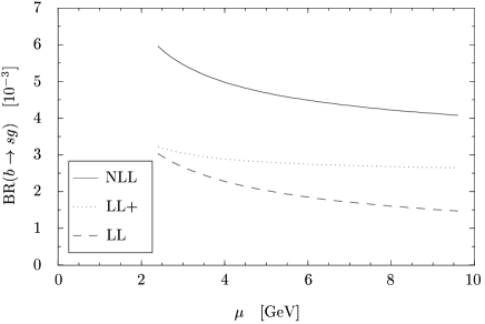
FIG. 5.: Branching ratio ${\cal B}(b\rightarrow sg)$ as a function of the scale $\mu$ in various approximations: The dashed and the solid lines show the LL and the NLL predictions, respectively; the dotted line is obtained by putting $r_{1}=r_{2}=r_{8}=\Gamma_{\rm{brems}}^{\rm{fin}}=0$ in the NLL expression for $\Gamma^{\rm{NLL}}(b\rightarrow sg)$ in eq. (41). See text.

The largest uncertainty due to the physical input parameters (other than $\mu$) on ${\cal B}(b\rightarrow sg)$ results from the charm quark mass. Varying $x_{c}=m_{c}/m_{b}$ between 0.27 and 0.31 and choosing $\mu=m_{b}$, the resulting uncertainty amounts to $\sim\pm 6\%$.

Acknowledgments: We would like to thank A. Ali, A. Kagan, A. Lenz, P. Minkowski, M. Neubert, and U. Nierste for helpful discussions.

REFERENCES

-
[1]
I. Bigi et al., Phys. Rev. Lett. 71, 496 (1993);
A. Manohar and M.B. Wise, Phys. Rev. D49, 1310 (1994);
B. Blok et al., Phys. Rev. D49, 3356 (1994);
T. Mannel, Nucl. Phys. B413, 396 (1994);
A. Falk, M. Luke, and M. Savage, Phys. Rev. D49, 3367 (1994). - [2] I. Bigi et al., Phys. Lett. B293, 430 (1992); 297 (1993) 477 (E).
- [3] G. Altarelli and S. Petrarca, Phys. Lett. B261, 303 (1991).
- [4] A. Lenz, U. Nierste and G. Ostermaier, Phys. Rev. D56, 7228 (1997).
- [5] A. Lenz, U. Nierste and G. Ostermaier, Phys. Rev. D59, 034008 (1999).
- [6] M. Ciuchini et al. Phys. Lett. B334, 137 (1994);
- [7] W. S. Hou, A. Soni and H. Steger, Phys. Rev. Lett. 59, 1521 (1987); W. S. Hou, Nucl. Phys. B308, 561 (1988).
- [8] H. Simma and D. Wyler, Nucl. Phys. B344, 283 (1990).
-
[9]
I. Bigi et al., Phys. Lett. B323, 408 (1994);
A. Falk, M.B. Wise, and I. Dunietz, Phys. Rev. D51, 1183 (1995);
I. Dunietz et al., Eur. Phys. J. C1, 211 (1998); H. Yamamoto, hep-ph/9912308. - [10] E. Bagan et al., Nucl. Phys. B432, 3 (1994); Phys. Lett. B 342, 362 (1995) [E:374, 363 (1996)]; E. Bagan et al., Phys. Lett. B 351, 546 (1995)
- [11] A. Golutvin, plenary talk given at the XXXth International Conference on High Energy Physics, Osaka, Japan, July 2000.
- [12] M. Neubert and C.T. Sachrajda, Nucl. Phys. B483, 339 (1997).
- [13] A. L. Kagan, Phys. Rev. D51, 6196 (1995).
- [14] A. L. Kagan and J. Rathsman, hep-ph/9701300.
- [15] M. Douadi, in: Proceedings of the International Conference on High Energy Physics, Jerusalem, Isreal, August 1997.
- [16] A. L. Kagan, in: Proceedings of the 2nd International Conference on B Physics and CP Violation, Honolulu, Hawaii, USA, March 1997 and hep-ph/9806266.
- [17] M. Neubert, in: Proceedings of the International Conference on High Energy Physics, Jerusalem, Isreal, August 1997 and hep-ph/9801269.
- [18] K. Chetyrkin, M. Misiak, and M. Münz, Phys. Lett. B400, 206 (1997); Nucl. Phys. B518, 473 (1998); Nucl. Phys. B520, 279 (1998).
-
[19]
K. Adel and Y.P. Yao, Phys. Rev. D49, 4945 (1994);
C. Greub and T. Hurth, Phys. Rev. D56, 2934 (1997);
M. Ciuchini et al., Nucl. Phys. B527, 21 (1998). - [20] C. Greub and P. Liniger, in preparation.
- [21] F.M. Borzumati and C. Greub, Phys. Rev. D58, 074004 (1998).
- [22] C. Greub, T. Hurth and D. Wyler, Phys. Lett. B380, 385 (1996); Phys. Rev. D54, 3350 (1996).
-
[23]
V.A. Smirnov, Renormalization and Asymptotic Expansions,
Birkhäuser Basel 1991;
E.E. Boos and A.I. Davydychev, Theor. Math. Phys. 89 1052 (1992);
N.I. Usyukina, Theor. Math. Phys. 79 (1989) 385, 22 211 (1975);
A. Erdelyi (ed.), Higher Transcendental Functions, McGraw New York 1953. - [24] Y. Nir, Phys. Lett. B221, 184 (1989).