Azimuthal angular dependence of decay lepton
in $e^{+}e^{-}\to t\bar{t}$

We discuss top quark production and its subsequent decay for searching new physics at lepton colliders. The angular dependence of the decay leptons is calculated including both QCD corrections and anomalous $\gamma/Z-t\bar{t}$ couplings. The off-diagonal spin basis for the top and anti-top quarks is shown to be useful to probe the anomalous couplings.

           hep-ph/0008065

           August 2000

1 Introduction

Since the discovery of the top quark, with a large mass [1], its properties have been widely discussed to obtain a better understanding of the electroweak symmetry breaking and to search for hints of physics beyond the standard model (SM). It has been known that top quarks decay before hadronization [2]. Therefore there will be sizable angular correlations between the decay products of the top quark and the spin of the top quark [3]. Based on this observation, it is expected that we can either test the SM or obtain some signal from new physics by investigating the angular distributions of the decay products from polarized top quarks. Applying the narrow width approximation to the top quarks, we can discuss the production process and decay process separately. There are many works on the spin correlations in top quark production at lepton and hadron colliders [4]. The angular dependence of the decay products from polarized top quark has also been discussed [3, 5].

Although it was common to use the helicity basis to decompose the top quark spin, it has been pointed out by Mahlon, Parke and Shadmi [6] that there is a more optimal decomposition of the top quark spin depending on the process and the center- of-mass energy $\sqrt{s}$. For instance, at a lepton collider, $\sqrt{s}$ of which is around several hundred GeV, it was shown [6, 7] that the so-called off-diagonal basis (ODB) is superior to other bases since top quarks (and/or anti-top quarks) are produced in an essentially unique spin configuration. The QCD one-loop radiative corrections to the spin correlation in top quark production are also investigated in ref.[8]. These radiative corrections induce an anomalous $\gamma/Z$ magnetic moment for the top quarks and allow for single, real gluon emission. Therefore, these effects possibly modify the tree level results. However what was found in ref.[8] is that the effect of the QCD corrections is mainly just the enhancement of the tree level result and does not change the spin configuration of produced top quarks (and/or anti-top quarks). This means that the ODB remains as a good basis even after including the QCD corrections.

On the other hand, there are also many detailed studies on the effects of new operators which might come from physics beyond the SM [9, 10]. The fact that the SM is consistent with the data within the present experimental accuracy tells us that the size of the effects of new physics is at most comparable to or smaller than the radiative corrections in the SM. Therefore, although the QCD correction to the top quark production is not so large, it should be included to detect these “small” signals from possible new physics beyond the SM.

In this article, we investigate the top quark production and its subsequent decay at lepton colliders both in the helicity and off-diagonal basis (ODB) including both the QCD correction and the assumed anomalous couplings for the $t\bar{t}-\gamma/Z$ interaction. For the angular distribution of the decay products, the interference between the amplitudes with different spin configurations plays an important role which disappears in the production cross section. We show that the azimuthal angular dependence in the top quark decay $t\to b\bar{l}\nu$ is one of the characteristics of the cross section in the ODB.

The article is organized as follows. In Section 2, we present the top quark production amplitudes including both QCD one-loop corrections and the anomalous couplings for the $t\bar{t}-\gamma/Z$ interaction. In Section 3, we analyze the angular dependence of the decay products from the top quark. Here we compare the results in the ODB with those in the helicity basis. Finally Section 4 contains the conclusions.

2 Top quark production with QCD corrections and anomalous couplings

The process we are considering now is, in principle, a very complicated $e^{-}e^{+}\to 6\ {\rm particles}$ one. However, the narrow width approximation for the top quark, which is valid for $\Gamma_{t}\ll m_{t}$ (1.02 $\leq\Gamma_{t}\leq$ 1.56 GeV for 160 $\leq m_{t}\leq$ 180 GeV), makes the situation very simple. Namely, we can separate the physics into the top production and the decay density matrices [11].

Let us first discuss the top quark production (density matrix). We assume a general form for the $t\bar{t}$-$Z/\gamma$ vertex as,

$$\Gamma^{V}_{\mu}=g^{V}\left\{\gamma_{\mu}\left[Q_{L}^{V}\omega_{-}+Q_{R}^{V}\omega_{+}\right]+\frac{(t-{\bar{t}})_{\mu}}{2m_{t}}\left[G_{L}^{V}\omega_{-}+G_{R}^{V}\omega_{+}\right]\right\}$$ (1)

where $t,\bar{t}$ are momenta of the top and top antiquarks, $m_{t}$ is the top mass, $\omega_{\pm}=(1\pm\gamma_{5})/2$ is the right/left projection operator, and $V=Z$ or $\gamma$. Here we use the normalization, $g_{\gamma}=g\sin\theta_{W}$ and $g_{Z}=g$ for the coupling constants with $g$ and $\theta_{W}$ the $SU(2)_{L}$ coupling and Weinberg angle, respectively. The form factor which will vanish in the zero electron mass limit is neglected. For the $e\bar{e}$-$Z/\gamma$ vertex, we use well established SM interaction. At the tree level in the SM, the coupling constants $G^{V}_{L,R}$ are zero and

$$Q^{\gamma}_{L}=Q^{\gamma}_{R}=Q_{t}\equiv\frac{2}{3},~{}~{}Q^{Z}_{L}=Q_{L}^{t}\equiv\frac{3-4\sin\theta_{W}^{2}}{6\cos\theta_{W}},~{}~{}Q^{Z}_{R}=Q_{R}^{t}\equiv-\frac{2\sin\theta_{W}^{2}}{3\cos\theta_{W}}.$$ (2)

The combination of form factors $G^{\gamma,Z}_{R}+G^{\gamma,Z}_{L}\equiv f_{2}^{\gamma,Z}$ is induced even at the one-loop level in the SM. Whereas, another combination $G^{\gamma,Z}_{R}-G^{\gamma,Z}_{L}\equiv if_{3}^{\gamma,Z}$ which is related to a CP violating interaction, called electric and weak dipole form factors (EDM and WDM) appears as, at least, the two-loop order effect. Thus they are negligibly small and non-zero value of $f_{3}^{\gamma,Z}$ is considered to be a contribution from new physics beyond the SM. We presume some non-zero value for $f_{3}^{\gamma,Z}$ and consider the top production.

To incorporate the QCD one-loop correction into this analysis, we utilize the fact [8] that the full one-loop QCD result can be reproduced quite accurately in the soft gluon approximation (SGA) by choosing an appropriate cut off $\omega_{\rm max}$ for the soft gluon energy. There, the formula $\omega_{\rm max}=\left(\sqrt{s}-2m_{t}\right)/5$ was suggested. The difference between the SGA using this $\omega_{\rm max}$ and the full one-loop correction is smaller than the expected size of the two-loop corrections. In the SGA, all QCD effects can be absorbed into the modified $t\bar{t}$-$Z/\gamma$ vertex, eq.(1), using the two universal functions ${\cal A}$ and ${\cal B}$.

$$Q_{L}^{\gamma} = Q_{R}^{\gamma}\,\equiv\,Q^{\gamma}=Q_{t}\,(1+\hat{\alpha}_{s}\,{\cal A}),$$

$$Q_{L}^{Z} = Q_{L}^{t}\,(1+\hat{\alpha}_{s}\,{\cal A})+(Q_{L}^{t}-Q_{R}^{t})\,\hat{\alpha}_{s}\,{\cal B}\ ,$$ (3)

$$Q_{R}^{Z} = Q_{R}^{t}\,(1+\hat{\alpha}_{s}\,{\cal A})-(Q_{L}^{t}-Q_{R}^{t})\,\hat{\alpha}_{s}\,{\cal B}\ .$$

and

$$G_{L,R}^{\gamma}=Q_{t}\,\hat{\alpha}_{s}\,{\cal B},\quad G_{L,R}^{Z}=\frac{Q_{L}^{t}+Q_{R}^{t}}{2}\,\hat{\alpha}_{s}\,{\cal B}\ .$$ (4)

where the strong coupling constant is $\hat{\alpha}_{s}\equiv\frac{C_{2}(R)}{4\pi}\alpha_{s}=\frac{C_{2}(R)}{(4\pi)^{2}}g^{2}$ with $C_{2}(R)=\frac{4}{3}$ for SU(3) of color. As mentioned before, the one-loop QCD correction does not contribute to the combination $G^{\gamma,Z}_{R}-G^{\gamma,Z}_{L}$. Since we assume an anomalous coupling to this combination, eq.(4) is modified to be,

$$G_{L/R}^{\gamma} = Q_{t}\,\hat{\alpha}_{s}\,{\cal B}\mp\frac{i}{2}f_{3}^{\gamma}\ ,$$

$$G_{L/R}^{Z} = \frac{Q_{L}^{t}+Q_{R}^{t}}{2}\,\hat{\alpha}_{s}\,{\cal B}\ \mp\frac{i}{2}f_{3}^{Z}.$$ (5)

The “renormalized” form factors ${\cal A}$ and ${\cal B}$ read after multiplying the wave function renormalization factor (we employ the on-shell renormalization scheme),

$${\rm Re}{\cal A} = \left(\frac{1+\beta^{2}}{\beta}\ln\frac{1+\beta}{1-\beta}-2\right)\ln\frac{4\omega_{\rm max}^{2}}{m_{t}^{2}}-4+\frac{2+3\beta^{2}}{\beta}\ln\frac{1+\beta}{1-\beta}$$ (6)

$$+ \frac{1+\beta^{2}}{\beta}\left\{\ln\frac{1-\beta}{1+\beta}\left(3\ln\frac{2\beta}{1+\beta}+\ln\frac{2\beta}{1-\beta}\right)+4{\rm Li}_{2}\left(\frac{1-\beta}{1+\beta}\right)+\frac{1}{3}\pi^{2}\right\}\ ,$$

$${\rm Im}{\cal A} = \pi\,\left(-3\beta+\frac{1+\beta^{2}}{\beta}\ln\frac{4\beta^{2}}{1-\beta^{2}}-\frac{1+\beta^{2}}{\beta}\ln\frac{\lambda^{2}}{m_{t}^{2}}\right)\ ,$$

$${\rm Re}{\cal B} = \frac{1-\beta^{2}}{\beta}\ln\frac{1+\beta}{1-\beta}\ ,$$ (7)

$${\rm Im}{\cal B} = \pi\,\frac{\beta^{2}-1}{\beta}\ ,$$

where $\beta$ is the speed of the produced top (anti-top) quark. In the form factor ${\cal A}$ eq.(6), we have already took into account the contribution from the real gluon emission. Therefore, there is no infrared singularity in the real part and instead there appears the soft gluon cut-off $\omega_{\rm max}$. We have introduced an infinitesimal mass $\lambda$ for the gluon to avoid the infrared singularity which remains in the imaginary part of ${\cal A}$. However it will be shown that the imaginary part of ${\cal A}$ does not contribute to any observable within our approximation which keep only the linear terms in $\alpha_{s}$ and $f_{3}^{\gamma,Z}$.

Before presenting the production amplitudes, let us define the spin basis according to ref. [6]. In this paper, we consider the case in which the spin of the top quark and anti-top quark in the production plane. The spins of the top and anti-top quarks are parameterized by $\xi$ as given in Fig.1. The top quark spin is decomposed along the direction ${\bf s}_{t}$ in the rest frame of the top quark which makes an angle $\xi$ with the anti-top quark momentum in the clockwise direction. Similarly, the anti-top quark spin states are defined in the anti-top rest frame along the direction ${\bf s}_{\bar{t}}$ having the same angle $\xi$ from the direction of the top quark momentum. The state $t_{\uparrow}\,\bar{t}_{\uparrow}\,(t_{\downarrow}\,\bar{t}_{\downarrow})$ refers to a top with spin in the $+{\bf s}_{t}\,(-{\bf s}_{t})$ direction in the top rest frame and an anti-top with spin $+{\bf s}_{\bar{t}}\,(-{\bf s}_{\bar{t}})$ in the anti-top rest frame. Note that the value $\cos\xi=-1$ corresponds to the helicity state. For the initial leptons, we use the helicity basis with the notation $e^{+}_{R,L}$ and $e^{-}_{R,L}$, where the subscripts $R,L$ denote the helicities of the particles.

Figure 1: The generic spin basis for the top (anti-top) quark in its rest frame. ${\bf s}_{t}$ (${\bf s}_{\bar{t}}$) is the top (anti-top) spin axis.

Now, the production amplitudes of top quark pairs in $e^{-}_{L}e^{+}_{R}$ annihilation turns out to be written in the following general forms in the zero momentum frame (ZMF),

$$M(e_{L}^{-}e_{R}^{+}\rightarrow t_{\uparrow}\bar{t}_{\uparrow},t_{\downarrow}\bar{t}_{\downarrow}) = \mp 4\pi\alpha\left[\left({A}_{LR}-{C}_{LR}\right)\cos\xi-{B}_{LR}\sin\xi\pm i{E}_{LR}\right]\ ,$$ (8)

$$M(e_{L}^{-}e_{R}^{+}\rightarrow t_{\uparrow}\bar{t}_{\downarrow},t_{\downarrow}\bar{t}_{\uparrow}) = \ \ 4\pi\alpha\left[\left({A}_{LR}-{C}_{LR}\right)\sin\xi+{B}_{LR}\cos\xi\pm{D}_{LR}\right]\ ,$$ (9)

employing an appropriate phase convention for spinors [7, 9]. $\alpha$ is the QED structure constant. The coefficients ${A}_{LR}$ , ${B}_{LR}$ ${D}_{LR}$ and ${E}_{LR}$ are given by,

$${A}_{LR} = \frac{1}{2}\,\Bigl{[}({f}_{LL}+{f}_{LR})\sqrt{1-\beta^{2}}\sin\theta\Bigr{]}\ ,$$

$${B}_{LR} = \frac{1}{2}\,\Bigl{[}{f}_{LL}(\cos\theta+\beta)+{f}_{LR}(\cos\theta-\beta)\Bigr{]}\ ,$$

$${C}_{LR} = \frac{1}{2}\,(h_{LL}+h_{LR})\frac{\beta^{2}\sin\theta}{\sqrt{1-\beta^{2}}}\ ,$$ (10)

$${D}_{LR} = \frac{1}{2}\,\Bigl{[}{f}_{LL}(1+\beta\cos\theta)+{f}_{LR}(1-\beta\cos\theta)\Bigr{]}\ ,$$

$${E}_{LR} = \frac{-i}{2}(h_{LL}-h_{LR})\frac{\beta\sin\theta}{\sqrt{1-\beta^{2}}}\ ,$$

with

$${f}_{IJ} = -Q^{\gamma}+\frac{Q^{e}_{I}\,Q^{Z}_{J}}{\sin^{2}\theta_{W}}\frac{s}{s-M_{Z}^{2}}\ ,$$

$$h_{IJ} = -G^{\gamma}_{J}+\frac{Q^{e}_{I}\,G^{Z}_{J}}{\sin^{2}\theta_{W}}\frac{s}{s-M_{Z}^{2}}\ ,$$ (11)

where the angle $\theta$ is the scattering angle of the top quark with respect to the electron in the ZMF. $M_{Z}$ is the Z-boson mass and we neglect the $Z$ width since it is negligible in the region of center-of-mass energy $\sqrt{s}$ far above the production threshold for top quarks. $I,J\in(L,R)$ and $Q^{e}_{I}$ is the electron coupling to the Z boson given by,

$$Q^{e}_{L}=\frac{2\sin^{2}\theta_{W}-1}{2\cos\theta_{W}}\quad,\quad Q^{e}_{R}=\frac{\sin^{2}\theta_{W}}{\cos\theta_{W}}\ .$$

In eq.(10), ${C}_{LR}$ is proportional to $f_{2}^{\gamma,Z}$ and the contribution from CP violating form factors $f_{3}^{\gamma,Z}$ enter through ${E}_{LR}$ only. The contributions from $f_{2}^{\gamma,Z}$, WDM and EDM form factors $f_{3}^{\gamma,Z}$, are enhanced when $\beta$ becomes large, and become zero for $\beta\to 0$. The amplitudes for $e^{-}_{R}e^{+}_{L}$ can be obtained by interchanging $R$ and $L$ as well as $\uparrow$ and $\downarrow$ in Eqs.(8)–(11).

At the tree level in the SM (${\cal A}={\cal B}=f_{3}=0$), the coefficients ${C}_{LR}$ and ${E}_{LR}$ are zero and other coefficients become real in eqs.(8,9). The ODB for the process $e^{-}_{L}e^{+}_{R}\rightarrow t\bar{t}$ is defined by,

$$\tan\xi=\left.\frac{{A}_{LR}}{{B}_{LR}}\right|_{\rm tree}\ ,$$

which makes the like-spin configurations $t_{\uparrow}\bar{t}_{\uparrow}$ and $t_{\downarrow}\bar{t}_{\downarrow}$ be zero. The up-down ($t_{\uparrow}\bar{t}_{\downarrow}$) configuration dominates the cross sections in the ODB whereas the down-up ($t_{\downarrow}\bar{t}_{\uparrow}$) is numerically negligible, less than $1\%$ of the total cross section.

The problem now is how to detect the anomalous coupling in the top quark events. It is easily understood that the effects of the anomalous coupling on the top quark production cross sections should be small and undetectable because (1) the anomalous coupling is assumed to be comparable to or smaller than the QCD correction in size and we already know the QCD correction itself to be very small and (2) the interference terms disappear in the production cross sections. Therefore we consider the angular distribution of top decay products which depends on the interferences between various amplitudes.

3 Decay distribution with anomalous coupling

In the decay process, we assume V-A interaction of the SM in $t$-$b$-$W$ vertex. We employ the semi-leptonic decay, $t\to bW\to b\bar{l}\nu$ for simplicity. Neglecting the mass of the final state fermions, the decay amplitude $D_{s_{t}}$ (for $t_{s_{t}}\to b\bar{l}\nu$) is known to be given by

$$D_{\uparrow}=\frac{2g^{2}V_{tb}\sqrt{b\cdot\nu~{}m_{t}E_{\bar{l}}}}{2\nu\cdot\bar{l}-M_{W}^{2}+iM_{W}\Gamma_{W}}\cos\frac{\theta_{\bar{l}}}{2}\ ,\ D_{\downarrow}=\frac{2g^{2}V_{tb}\sqrt{b\cdot\nu~{}m_{t}E_{\bar{l}}}}{2\nu\cdot\bar{l}-M_{W}^{2}+iM_{W}\Gamma_{W}}\sin\frac{\theta_{\bar{l}}}{2}e^{-i\phi_{\bar{l}}}\ ,$$ (12)

where the names of final particles are used as substitute for their momenta. $M_{W}(\Gamma_{W})$ and $V_{tb}$ are the mass (width) of the W boson and the Cabbibo–Kobayashi–Maskawa matrix.

Figure 2: The definition of polar and azimuthal angles.

The polar and azimuthal angles of the $\bar{l}$ momentum ($\theta_{\bar{l}},\phi_{\bar{l}}$) are defined in the top quark rest frame, in which $z$-axis coincides with the chosen spin axis $s_{t}$ and the $x-z$ plane is the production plane, Fig.2. We have a similar expression $\bar{D}_{\uparrow\downarrow}$ also for the anti-top quark decay.

Now, the differential cross-section for the process $e^{-}e^{+}\to t\bar{t}$ followed by the decays $t\to X_{t}\,,\,\bar{t}\to\bar{X}_{t}$ is described in terms of the production and decay density matrices $\rho_{s_{t}\bar{s}_{t},s^{\prime}_{t}\bar{s}^{\prime}_{t}}$  ,  $\tau_{s_{t}s^{\prime}_{t}}$ and $\bar{\tau}_{\bar{s}_{t}\bar{s}^{\prime}_{t}}$ as,

$$d\sigma\left(e^{-}e^{+}\to t\bar{t}\to X_{t}\bar{X}_{t}\right)\propto\sum_{s_{t},\bar{s}_{t},s^{\prime}_{t},\bar{s}^{\prime}_{t}}\rho_{s_{t}\bar{s}_{t},s^{\prime}_{t}\bar{s}^{\prime}_{t}}\tau_{s_{t}s^{\prime}_{t}}\bar{\tau}_{\bar{s}_{t}\bar{s}^{\prime}_{t}}dL\ ,$$ (13)

where $dL$ is the phase space of the final particles and the density matrices can be obtained from eqs.(8), (9) and (12) [11].

$$\rho_{s_{t}\bar{s}_{t},s^{\prime}_{t}\bar{s}^{\prime}_{t}} = M_{s_{t}\bar{s}_{t}}M^{\ast}_{s^{\prime}_{t}\bar{s}^{\prime}_{t}}\ ,$$

$$\tau_{s_{t}s^{\prime}_{t}} = D_{s_{t}}D^{\ast}_{s^{\prime}_{t}}\propto\left(\begin{array}[]{cc}1+\cos\theta_{\bar{l}}&\sin\theta_{\bar{l}}\,e^{i\phi_{\bar{l}}}\\ \sin\theta_{\bar{l}}\,e^{-i\phi_{\bar{l}}}&1-\cos\theta_{\bar{l}}\\ \end{array}\right)_{s_{t}s^{\prime}_{t}}\ .$$ (16)

$\bar{\tau}_{\bar{s}_{t}\bar{s}^{\prime}_{t}}$ is also given by the similar expression. When we calculated the production density matrix, we have kept only terms which are linear in $\alpha_{s}$ and $f_{3}^{\gamma,Z}$ for the consistency of our approximation. Within this approximation, the factor $1+\hat{\alpha}_{s}A$ can be effectively factorized from the amplitudes as a multiplicative factor. Therefore its imaginary part which has the infrared divergence does not contribute to the production density matrix.

Here we take an advantage of the freedom for the choice of the spin basis to detect the effect of the anomalous couplings [7, 9]. Note that the differential cross section itself is (should be) independent of the choice of the spin basis. However, the “choice of the variables”  can depend on the spin basis. We have calculated the angular distribution of $\bar{l}$ in the top quark decay after integrating out other variables,

$$\frac{d\sigma\left(e_{L}^{-}e_{R}^{+}\to t\bar{t}\to\bar{l}+X\right)}{d\cos\theta d\cos\theta_{\bar{l}}d\phi_{\bar{l}}}\ .$$

All input masses and coupling constants used in the numerical computations are the central values as reported in the 1998 Review of Particle Properties [12]. We plot the $\theta_{\bar{l}}-\phi_{\bar{l}}$ correlations both in the helicity (Fig.3) and the off-diagonal basis (Fig.4). We set $\sqrt{s}=400$ GeV and assume $f_{3}^{\gamma,Z}=0.2$ just for an illustration. The both figures are for $\cos\theta=0$. However the pattern of the correlation is essentially the same for all scattering angles. One can see that it is very hard to identify the effects of the anomalous couplings in Fig. 3. This situation changes drastically if we take the ODB (Fig. 4). As the SM produces almost no azimuthal angular dependence in this basis (although the QCD corrections produce some dependence, it is numerically negligible), we can recognize the effect of the anomalous coupling as a deviation from the flat distribution.

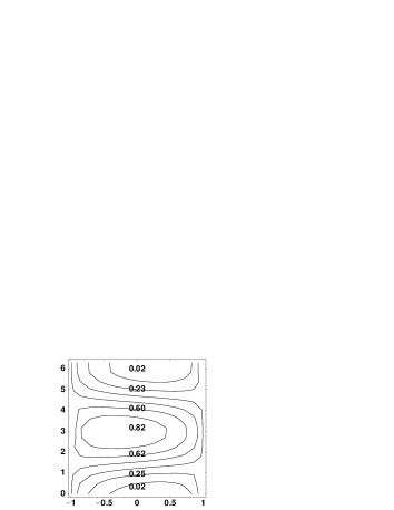
Figure 3: The double differential cross section $d\sigma/d\cos\theta_{\bar{l}}d\phi_{\bar{l}}$ in the helicity basis. The left (right) figure correspond to the cross section without (with) the anomalous $f_{3}^{\gamma,Z}$ coupling. Vertical and horizontal axes correspond to the azimuthal $\phi_{\bar{l}}$ and the polar angle $\cos\theta_{\bar{l}}$, respectively.

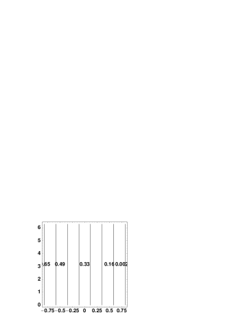
Figure 4: The double differential cross section in the off-diagonal basis. The left (right) figure correspond to the cross section without (with) the anomalous $f_{3}^{\gamma,Z}$ coupling. The axes are the same as in Fig.3

The above results are easily understood if one notices that the azimuthal angular dependence is caused by interference effects in a given spin basis. From eq.(16), the azimuthal angular dependence comes from the off diagonal $\uparrow\downarrow$ or $\downarrow\uparrow$ element of the decay density matrix. On the other hand, the production amplitudes, therefore the density matrix, take the following characteristic forms (see eqs.(8,9)) in the ODB,

$$M_{\uparrow\uparrow} \sim M_{\downarrow\downarrow}\sim{E}_{LR}\ ,$$

$$M_{\uparrow\downarrow} \sim {\rm finite}\ ,\ M_{\downarrow\uparrow}\sim 0\ ,$$

except small contributions from the QCD correction. This means that the azimuthal angular dependence receives significant contributions only from the elements,

$$\rho_{\uparrow\downarrow,\downarrow\downarrow}\ ,\quad\rho_{\downarrow\downarrow,\uparrow\downarrow}\ ,$$

of the production density matrix and it linearly depends on ${E}_{LR}$, namely $f_{3}^{\gamma,Z}$. The $\phi_{\bar{l}}$ dependence is controlled by the value of $f_{3}^{\gamma,Z}$. At the tree level, it has a simple form,

$${\rm Re}\,f_{3}^{\gamma,Z}\sin\,\phi_{\bar{l}}-{\rm Im}\,f_{3}^{\gamma,Z}\cos\,\phi_{\bar{l}}\ .$$

In order to show the effect of the $f_{3}^{\gamma,Z}$ more clearly, we partially integrate the cross section over the azimuthal angle and define the azimuthal asymmetry. Let $\sigma^{1,2}$ denote the partially integrated cross-sections over the azimuthal angle,

$$\sigma^{1}(\theta) = \int_{0}^{\pi}d\phi_{\bar{l}}\left(\frac{d\sigma}{d\cos\theta d\phi_{\bar{l}}}\right)\ ,$$

$$\sigma^{2}(\theta) = \int_{\pi}^{2\pi}d\phi_{\bar{l}}\left(\frac{d\sigma}{d\cos\theta d\phi_{\bar{l}}}\right)\ ,$$

where other variables have been integrated out already. We define the azimuthal asymmetry in order to pull out the effect of anomalous interactions,

$${\cal A}(\theta)=\frac{\sigma^{2}(\theta)-\sigma^{1}(\theta)}{\sigma^{2}(\theta)+\sigma^{1}(\theta)}.$$

We plot the asymmetry as a function of $\cos\theta$ in Fig.5 at $\sqrt{s}=400$ GeV for the $e^{-}_{L}e^{+}_{R}$ and $e^{+}_{L}e^{-}_{R}$ annihilation. We have assumed two cases for the anomalous couplings, ${\rm Re}\,f_{3}^{\gamma}={\rm Re}\,f_{3}^{Z}=0.2$ and ${\rm Re}\,f_{3}^{\gamma}=-{\rm Re}\,f_{3}^{Z}=0.2$.

Figure 5: Azimuthal asymmetry as a function of $\cos\theta$ in the off-diagonal basis.

In this figure, the dot-dashed line comes from the SM (with QCD corrections) and, the solid (dashed) line corresponds to the case ${\rm Re}\,f_{3}^{\gamma}={\rm Re}\,f_{3}^{Z}=0.2$ (${\rm Re}\,f_{3}^{\gamma}=-{\rm Re}\,f_{3}^{Z}=0.2$). At the SM tree level, the asymmetry is exactly zero and the QCD radiative corrections induce a numerically negligible asymmetry as shown in Fig.6. As explained before, the asymmetry linearly depends on the absolute value of $f_{3}^{\gamma,Z}$ and also their sign. In the case of $e^{-}_{L}e^{+}_{R}$, the effect of the anomalous interactions $f_{3}^{\gamma}$ and $f_{3}^{Z}$ are additive and have a larger asymmetry when their signs are the same. But when their signs are opposite, these effects become subtractive and lead to a smaller asymmetry. This feature changes in the case of $e^{+}_{L}e^{-}_{R}$. In the off-diagonal basis, the anomalous couplings produce the asymmetry of the order 10% for the values of the anomalous couplings we have chosen. In the helicity basis, however, the deviation from the SM is only around 1.5% since there exists some amount of asymmetry already in the SM. If we take the asymmetry by defining $\sigma^{1,2}$ as,

$$\sigma^{1}(\theta) = \left(\int_{0}^{\frac{\pi}{2}}+\int_{\frac{3\pi}{2}}^{2\pi}\right)\,d\phi_{\bar{l}}\left(\frac{d\sigma}{d\cos\theta d\phi_{\bar{l}}}\right)\ ,$$

$$\sigma^{2}(\theta) = \int_{\frac{\pi}{2}}^{\frac{3\pi}{2}}d\phi_{\bar{l}}\left(\frac{d\sigma}{d\cos\theta d\phi_{\bar{l}}}\right)\ ,$$

we can obtain information for ${\rm Im}\,f_{3}^{\gamma,Z}$.

Figure 6: Azimuthal asymmetry induced by the QCD correction in the off-diagonal basis for the $e^{-}_{L}e^{+}_{R}$ annihilation.

4 Conclusion

We have studied the top quark pair production and subsequent decays at lepton colliders. For a realistic next lepton collider, let us say $\beta\sim 0.5$, the off-diagonal basis is considered to be a good choice since the contribution from some spin states is zero or negligible even after including the QCD corrections and this small interference makes the correlations between decay products and the top spin very strong. Using this advantage, we analyzed the angular dependence of the decay product of the top quark including both the QCD corrections and the anomalous couplings. We have shown that the asymmetry amount to the order of 10% in the off-diagonal basis with chosen parameters which may be detectable.

Although we have considered the anomalous couplings only for the production process, the inclusion of new effects to the decay process and more detailed and/or realistic phenomenological analyses for various choices of the new interactions are straightforward exercises.

References

• [1] F. Abe et al., CDF Collab., Phys. Rev. Lett. 74 (1995) 2626.
S. Abachi et al., D0 Collab., Phys. Rev. Lett. 74 (1995) 2632.
• [2] I. Bigi, Y. Dokshitzer, V. Khoze, J. KΓΌhn and P. Zerwas, Phys. Lett. B181 (1986) 157.
• [3] J. H. KΓΌhn, Nucl. Phys. B237 (1984) 77.
M. JeΕΌabek and J. H. KΓΌhn, Phys. Lett. B329 (1994) 317; and references therein.
• [4] G. Mahlon and S. Parke, hep-ph/0001201;Β and references therein.
• [5] G.Β L.Β Kane, J.Β Pumplin and W.Β Repko, Phys. Rev. Lett. 41 (1978) 1689.
G.Β L.Β Kane, G.Β A.Β Ladinsky and C.Β -P.Β Yuan, Phys. Rev. D45 (1992) 124.
• [6] G. Mahlon and S. Parke, Phys. Rev. D53 (1996) 4886.
S. Parke and Y. Shadmi, Phys. Lett. B387 (1996) 199.
• [7] G. Mahlon and S. Parke, Phys. Lett. B411 (1997) 173.
• [8] J. Kodaira, T. Nasuno and S. Parke, Phys. Rev. D59 (1999) 014023.
• [9] T. Torma, hep-ph/9912281.
• [10] For recent articles, see e.g. S. M. Lietti and H. Murayama, hep-ph/0001304.
S. D. Rindani, hep-ph/0002006.
B. Grzadkowski and Z. Hioki, hep-ph/0003294; and references therein.
• [11] M. Jezabek and J. H. KΓΌhn, Nucl. Phys. B320 (1989)20.
A. Czarnecki, M. JeΕΌabek and J. H. KΓΌhn, ibid. B427 (1994) 3.
B. Lampe, in Prceedings of the International Symposium on QCD Corrections and New Physics, Hiroshima, Japan, 1997, edited by J.Kodaira, T.Onogi and K.Sasaki (World Scientific,Singapore,1998) (hep-ph/9801346, MPI-PHT Report No.98-07).
• [12] C. Caso et al, Eur. Phys. J. C3 (1998) 1.