Renormalons as dilatation modes in the functional space

A. BABANSKY and I. BALITSKY

Physics Department, Old Dominion University, Norfolk VA 23529

and

Theory Group, Jefferson Lab, Newport News VA 23606

e-mail: balitsky@jlab.org and babansky@jlab.org

Abstract

There are two sources of the factorial large-order behavior of a typical perturbative series. First, the number of the different Feynman diagrams may be large; second, there are abnormally large diagrams known as renormalons. It is well known that the large combinatorial number of diagrams is described by instanton-type solutions of the classical equations. We demonstrate that from the functional-integral viewpoint the renormalons do not correspond to a particular configuration but manifest themselves as dilatation modes in the functional space.

PACS numbers: 12.38.Cy, 11.15.Bt, 11.15.Kc

I Introduction

It is well known that the perturbative series in a typical quantum field theory is at best asymptotic: the coefficients in front of a typical perturbative expansion grow like $n!$ where n is the order of the perturbation series (see e.g. the book [1]). There are two sources of the $n!$ behavior which correspond to two different situations. In the first case all Feynman diagrams are $\sim 1$ but their number is large ($\sim n!$) [2]. In the second case, we have just one diagram but it is abnormally big – $\sim n!$ (the famous ‘t Hooft renormalon [3]). The first type of factorial behavior is not specific to a field theory; for example, it can be studied in the anharmonic-oscillator quantum mechanics. On the contrary, renormalon singularities can occur only in field theories with running coupling constant (for the review of the renormalons, see ref.[4] and references therein).

It is convenient to visualize the large-order behavior of perturbative series using the ’t Hooft picture of singularities[3]. Consider Adler’s function related to the polarization operator in QCD

$$D(q^{2})={4\pi^{2}}q^{2}{d\over dq^{2}}{1\over 3q^{2}}\Pi(q^{2}),$$ (1)

$$\Pi(q^{2})=\int\!dxe^{iqx}\int\!D\bar{\psi}D\psi DAj_{\mu}(x)j_{\mu}(0)e^{-S_{\rm QCD}}$$ (2)

Suppose we write down $D(q^{2})$ as a Borel integral

$$D(\alpha_{s}(q))=\int_{0}^{\infty}dtD(t)e^{-{4\pi\over\alpha_{s}(q)}t}$$ (3)

The divergent behavior of the original series $D(\alpha_{s}(q)$ is encoded in the singularities of its Borel transform shown in Fig.1.

         

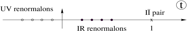
FIG. 1.: ’t Hooft picture of singularities in the Borel plane for QCD.

In QCD, we have two types of singularities: renormalons (ultraviolet or infrared) and instanton-induced singularities . The ultraviolet (UV) renormalons are located at $t=-{1\over b},{2\over b},{3\over b}...$ ($b=11-{2\over 3}n_{f}$). In terms of Feynman diagrams they come from the regions of hard momenta in renormalon bubble chain, see Fig. 2.

                 

FIG. 2.: Typical renormalon bubble chain diagrams for the polarization operator in QCD.

The infrared (IR) renormalons placed at $t={2\over b},{3\over b}...$ come from the region of soft momenta in the bubble chain diagrams. The instanton singularities are located at $t=1,2,3,...$ and they correspond to the large number of graphs which are summed up to the contribution of $I\bar{I}$ configurations in the functional space. The main result of this paper is that unlike the instanton-type singularities, the renormalons do not correspond to a particular configuration but manifest themselves as dilatation modes in the functional space.

The paper is organized as follows. In Section 2 we relate Borel representation to the functional integral along the instanton-antiinstanton valley in the double-well quantum mechanics. In Section 3 we describe the conformal valley in QCD and discuss the relation between valleys and Borel representation in the field theories with running coupling constant. Sect. 4 and 5 are devoted to the interpretation of IR and UV renormalons as dilatation modes of the valley. In the last section we discuss general aspects of our approach and outline the direction of the future work.

II Valleys and Borel plane in quantum mechanics

The interpretation of renormalons as dilatation modes is based upon the similarity of the functional integral in the vicinity of a valley in the functional space[6] to the Borel representation (2). At first, we will consider the quantum mechanical example without renormalons and then demonstrate that in a field theory the same integral along the valley leads to renormalon singularities. With QCD in view, we consider the double-well anharmonic oscillator described by the functional integral

$$Z~{}=\int\!D\phi e^{-{S(\phi)\over g^{2}}}$$ (4)

where

$$S(\phi)=\int\!dt\left({\dot{\phi}^{2}\over 2}+{\phi^{2}(1-\phi)^{2})\over 2}\right)$$ (5)

The large-order behavior in this model is determined by the instanton-antiinstanton ($I\bar{I}$) configuration. The $I\bar{I}$ valley for the double-well system may be chosen as

$$f_{\alpha}(t-\tau)={1\over 2}\tanh{t-\tau+\alpha\over 2}-{1\over 2}\tanh{t-\tau-\alpha\over 2}$$ (6)

It satisfies the valley equation[8][9]

$${12\over\xi^{2}}w_{\alpha}(t)f^{\prime}_{\alpha}(t)=L_{\alpha}(t)$$ (7)

where $\xi\equiv e^{\alpha}$, $f^{\prime}_{\alpha}\equiv{\partial\over\partial\alpha}f_{\alpha}$, and $L_{\alpha}(t)=\left.{\delta S\over\delta\phi}\right|_{\phi=f_{\alpha}(t)}$. Here $w_{\alpha}(t)={\xi\over 4}\sinh\alpha(\cosh\alpha\cosh t+1)^{-1}$ is the measure in the functional space so $(f,g)\equiv\int dtw_{\alpha}(t)f(t)g(t)$. The valley (6) connects two classical solutions: the perturbative vacuum at $\alpha=0$ and the infinitely separated $I\bar{I}$ pair at $\alpha\rightarrow\infty$. The $I\bar{I}$ separation $\alpha$ and the position of the $I\bar{I}$ pair $\tau$ are the two collective coordinates of the valley. In order to integrate over the small fluctuations near the configuration (6), we introduce two $\delta$-functions $\delta(\phi(t)-f_{\alpha}(t-\tau),\dot{f}_{\alpha}(t-\tau))$ and $\delta(\phi(t)-f_{\alpha}(t-\tau),{f}^{\prime}_{\alpha}(t-\tau))$ restricting the integration along the two collective coordinates. Following the standard procedure (Faddeev-Popov trick), we insert

$$1=\int d\alpha\left[(f^{\prime}_{\alpha},f^{\prime}_{\alpha})+(\phi-f_{\alpha},f^{\prime}_{\alpha}+{w^{\prime}\over w}f_{\alpha})\right]\delta(\phi-f_{\alpha},f^{\prime}_{\alpha})$$ (8)

and

$$1=\int d\tau\left[(\dot{f}_{\alpha},\dot{f}_{\alpha})+(\phi-f_{\alpha},\dot{f}_{\alpha}+{\dot{w}\over w}f_{\alpha})\right]\delta(\phi-f_{\alpha},\dot{f}_{\alpha})$$ (9)

in the functional integral (4). Next steps are the shift $\phi(t)\rightarrow\phi(t)+f_{\alpha}(t-\tau)$, expansion in quantum deviations $\phi(t)$ and the gaussian integration in the first nontrivial order in perturbation theory. After the shift, the the linear term in the exponent $\int dt\phi(t)L_{\alpha}(t)$ is disabled due to the valley equation (7) (recall $\delta(\phi,f^{\prime}_{\alpha})$ in the integrand coming from eq. (8)) so the functional integral (4) for the vacuum energy in the leading order in $g^{2}$ reduces to

$$T\int\!d\alpha\!\int\!D\phi(f^{\prime}_{\alpha},f^{\prime}_{\alpha})(\dot{f}_{\alpha},\dot{f}_{\alpha})\delta(\phi,f^{\prime}_{\alpha})\delta(\phi,\dot{f}_{\alpha})e^{-{1\over g^{2}}\left[S_{\alpha}+{1\over 2}\int\!dt\phi(t)\Box_{\alpha}\phi(t)\right]}+O(g^{2}).$$ (10)

Here T (the total ”volume” in one space-time dimension) is the result of trivial integration over $\tau$, $\Box_{\alpha}=-\partial^{2}+1-6f_{\alpha}(1-f_{\alpha})$ is the operator of second derivative of the action and

$$S_{\alpha}\equiv S(\xi)={6\xi^{4}-14\xi^{2}\over(\xi^{2}-1)^{2}}-{17\over 3}+{12\xi^{2}+4\over(\xi^{2}-1)^{3}}\ln\xi$$ (11)

is the action of $I\bar{I}$ valley. Performing Gaussian integrations we get

$$T{1\over g^{2}}\int_{0}^{\infty}\!d\alpha e^{-{1\over g^{2}}S_{\alpha}}F(\alpha),$$ (12)

$$F(\alpha)={(\det\Box_{\alpha})^{-1/2}(f^{\prime}_{\alpha},f^{\prime}_{\alpha})(\dot{f}_{\alpha},\dot{f}_{\alpha})\over\left(f^{\prime}_{\alpha},\Box^{-1}_{\alpha}w_{\alpha}f^{\prime}_{\alpha}\right)^{1/2}\left(\dot{f}_{\alpha},\Box^{-1}_{\alpha}w_{\alpha}\dot{f}_{\alpha}\right)^{1/2}}.$$ (13)

At $\alpha\rightarrow\infty$ we have the widely separated $I$ and $\bar{I}$. In this case, the determinant of the $I\bar{I}$ configuration factorizes into a product of two one-instanton determinants (with zero modes excluded) so that $F(\alpha)\rightarrow{\rm const}$ at $\alpha\rightarrow\infty$. The divergent part of the integral (12) corresponds to the second iteration of the one-instanton contribution to the vacuum energy, therefore it must be subtracted from the $I\bar{I}$ contribution to $E_{\rm vac}$:

$$g^{2}E_{\rm vac}(g^{2})=\int\!d\alpha\!\left(e^{-{1\over g^{2}}S_{\alpha}}F(\alpha)-e^{-{1\over g^{2}}2S_{I}}F(\infty)\right)$$ (14)

where $S_{I}$ is the one-instanton action. Since $S_{\alpha}$ is a monotonous function of $\alpha$ one can invert Eq. (11) and obtain

$$g^{2}E_{\rm vac}(g^{2})=\int_{0}^{2S_{I}}\!dSe^{-{1\over g^{2}}S}F(S)\left({1\over S-2S_{I}}\right)_{+}$$ (15)

which has the desired form of the Borel integral (1) for the vacuum energy. Thus the leading singularity for $E_{\rm vac}(S)$ is $F(2S_{I})/(S-2S_{I})$. Note that our semiclassical calculation does not give the whole answer for the Borel transform of vacuum energy ($F(S)\not\!=E_{\rm vac}(S)$ in general) since we threw away the higher quantum fluctuations around the $I\bar{I}$ pair in Eq. (10) yet it determines the the leading singularity in the Borel plane.

III $I\bar{I}$ valley and Borel integral in QCD

The situation with the instanton-induced asymptotics of perturbative series in a field theory such as QCD is pretty much similar to the case of quantum mechanics with one notable exception: in QCD there is an additional dimensional parameter – the overall size of the $I\bar{I}$ configuration $\rho$. The classical $I\bar{I}$ action does not depend on this parameter but the quantum determinant does, leading to the replacement

$$e^{-{1\over g^{2}}S}\rightarrow e^{-{1\over g^{2}(\rho)}S}$$ (16)

so the Borel integrand have the following generic form

$$F(S)\sim\int d\rho e^{-{1\over g^{2}(\rho)}S}{\cal F}(\rho)$$ (17)

The divergence of this integral at either large or small $\rho$ determines the position of singularities of $F(s)$. We will demonstrate (by purely dimensional analysis) that ${\cal F}(\rho)\sim\rho^{-5}$ at $\rho\rightarrow\infty$ and ${\cal F}(\rho)\sim\rho$ at $\rho\rightarrow 0$ leading to the IR renormalon at $S={32\pi^{2}\over b}$ and the UV renormalon at $S=-{16\pi^{2}\over b}$, respectively .

The $I\bar{I}$ valley in QCD[8] can be chosen as a conformal transformation of the spherical configuration

$$A_{\mu}(x)=-i{\bar{\sigma}_{\mu}x-x_{\mu}\over x^{2}}f_{\alpha}(t)$$ (18)

with $t=\ln x^{2}/d^{2}$ where $d$ is an arbitrary scale. (We use the notations $x\equiv x_{\mu}\sigma_{\mu},~{}~{}\bar{x}\equiv x_{\mu}\bar{\sigma}_{\mu}$ where $\sigma_{\mu}=(1,-i\vec{\sigma}),~{}~{}\bar{\sigma}_{\mu}=(1,i\vec{\sigma})$). To obtain the $I\bar{I}$ configuration with arbitrary sizes $\rho_{1},\rho_{2}$ and separation $R$ one performs shift $x\rightarrow x-a$, inversion $x\rightarrow{d^{2}\over x^{2}}x$ and second shift $x\rightarrow x-x_{0}$ (see Fig. 3).

                 

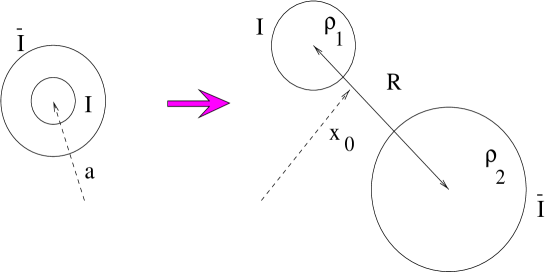
FIG. 3.: Conformal $I\bar{I}$ valley in QCD.

The resulting valley is the sum of the $I$ and $\bar{I}$ in the singular gauge in the maximum attractive orientation plus the additional term (which is small at large $I\bar{I}$ separations)

$$A^{v}_{\mu}(x)=A^{I}_{\mu}(x-x_{0})+A^{\bar{I}}_{\mu}(x-x_{0})+B_{\mu}(x-x_{0})$$ (19)

where

$$A^{I}_{\mu}(x) = -i\rho_{1}^{2}{\sigma_{\mu}\bar{x}-x_{\mu}\over x^{2}(x^{2}+\rho_{1}^{2})}$$ (20)

$$A^{\bar{I}}_{\mu}(x) = -i\rho_{2}^{2}{R\bar{\sigma}_{\mu}(x-R)\bar{R}-(x-R)_{\mu}\over R^{2}(x-R)^{2}((x-R)^{2}+\rho_{2}^{2})}.$$ (21)

The explicit expression for $B_{\mu}$ can be found in [9]. The action of the $I\bar{I}$ valley (19) is equal to the action of the spherical configuration (18) given by (11):

$$S^{v}(z)=48\pi^{2}S(\xi),~{}~{}\xi=z+\sqrt{z^{2}-1},$$ (22)

where the ”conformal parameter” $z$ is given by

$$z=(\rho_{1}^{2}+\rho_{2}^{2}+R^{2})/(2\rho_{1}\rho_{2}).$$ (23)

Let us now calculate the polarization operator (1) in the valley background. The collective coordinates are the sizes of instantons $\rho_{i}$, separation $R$, overall position $x_{0}$ and the orientation in the color space (the valley of a general color orientation has the form ${\cal O}_{ab}A^{v}_{b}$ where ${\cal O}$ is an arbitrary $SU(3)$ matrix). The structure of Gaussian result for the polarization operator in the valley background is

$$\int_{0}^{\infty}\!{d\rho_{1}d\rho_{2}\over\rho_{1}^{5}\rho_{2}^{5}}d^{4}Rd^{4}x_{0}d{\cal O}\Pi^{v}(q){1\over g^{17}}e^{-{S^{v}(z)\over g^{2}}}\Delta(\rho_{i},R)$$ (24)

where 17 is a number of the collective coordinates . Here $\Pi^{v}(q)$ is a Fourier transform of

$$\Pi^{v}(x)=(\sum e_{q}^{2}){\rm Tr}\gamma_{\mu}G(x,0)\gamma_{\mu}G(0,x)$$

where $G(x,y)$ is the Green function in the valley background. The factor $\Delta(\rho_{i},R)$ in Eq. (24) is the quantum determinant - the result of Gaussian integrations near the valley (19) with the additional factors due to the restricted integrations along the collective coordinates (cf. eq. (13)). For our purposes, it is convenient to introduce the conformal parameter $z$ and the average size $\rho=\sqrt{\rho_{1}\rho_{2}}$ as the collective coordinates in place of $\rho_{1}$ and $\rho_{2}$. We have

$$\int\!dz{d\rho\over\rho^{9}}d^{4}Rd^{4}x_{0}\Pi^{v}(q){1\over g^{17}(\rho)}F(z,R^{2}/\rho^{2})e^{-{S^{v}(z)\over g^{2}(\rho)}}$$ (25)

where $F(z,R^{2}/\rho^{2})$ contains $\theta(z-1-{R^{2}\over 2\rho^{2}})$ (see Eq. (23)). We have included in $F$ the trivial integral over color orientation which gives the volume of $SU(3)$ group.

The main effect of the quantum determinant $\Delta$ is the replacement of the bare coupling constant $g^{2}$ in Eq. (24) by the effective coupling constant $g^{2}(\rho)$ so the remaining function $F$ is the (dimensionless) function of the ratio $R^{2}/\rho^{2}$ and the conformal parameter. This is almost evident from the renormalizability of the theory since the only dimensional parameters are $\rho$ and $R$. Formally, one can prove that rescaling of the configuration by factor $\lambda$ (so that $\rho\rightarrow\lambda\rho$ and $R\rightarrow\lambda R$) leads at the one-loop level to multiplication of the determinant by a factor $\lambda^{bS^{v}(z)/8\pi^{2}}$ due to conformal anomaly (see Appendix).

IV IR renormalon from the dilatation mode of the $I\bar{I}$ valley

Consider the singularities of the integral (25). The function $F(z,R^{2}/\rho^{2})$ is non-singular since the singularity in $\Phi$ ($\equiv$ singularity in $\Delta$) would mean a non-existing zero mode in quantum determinant. Moreover, the integration over $R$ is finite due to $\theta(z-1-{R^{2}\over 2\rho^{2}})$ indicating that the only source of singularity at finite $z$ is the divergence of the $\rho$ integral at either large or small $\rho$. (At $z\rightarrow\infty$, in a way similar to the derivation of Eq. (15) we obtain the first instanton-type singularity located at $t=1$[10]).

Let us demonstrate that the singularity of the integral (25) at large $\rho\gg{1\over q}$ corresponds to the IR renormalon. The polarization operator $\Pi(q)$ in the background of the large-scale vacuum fluctuation reduces to[11] (see Fig. 3)

$$\Pi(q)=\int d^{4}xe^{iqx}\langle j_{\mu}(x)j_{\mu}(0)\rangle_{A}\rightarrow-{\sum e_{q}^{2}\over 16\pi^{2}}\Big{(}{G^{2}(0)\over q^{2}}+c\alpha_{s}{G^{3}(0)\over q^{4}}+...\Big{)}$$ (26)

where $G^{2}\equiv 2{\rm Tr}G_{\xi\eta}G_{\xi\eta}$, $G^{3}\equiv 2{\rm Tr}G_{\xi\eta}G_{\eta\sigma}G_{\sigma\xi}$, and $c$ is an (unknown) constant. (The coefficient in front of $G^{3}$ vanishes at the tree level[13]).

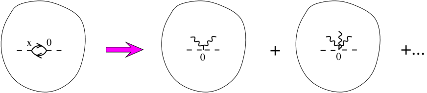
FIG. 4.: Expansion of the polarization operator in large-scale external fields.

Consider the leading term in this expansion; since the field strength for the valley configuration (19) depends only on $x-x_{0}$

$$\int d^{4}x_{0}{\rm Tr}G^{v}_{\xi\eta}(0)G^{v}_{\xi\eta}(0)=4S^{v}(z),$$ (27)

the intergal (25) takes the form

$${1\over q^{2}}\int_{1}^{\infty}dz\int_{0}^{\infty}{d\rho\over\rho^{9}}d^{4}R{1\over g^{17}(\rho)}F(z,{R^{2}/\rho^{2}})e^{-{S^{v}(z)\over g^{2}(\rho)}}$$ (28)

where we have included the factor ${1\over 4\pi^{2}}\sum e_{q}^{2}S^{v}(z)$ in $F$. The (finite) integration over $R$ can be performed resulting in an additional dimensional factor $\rho^{4}$:

$$\int d^{4}RF(\rho,z,R)=\rho^{4}\Phi(z)$$

where the function $\Phi$ is dimensionless so it can depend only on $z$. Finally, we get

$${1\over q^{2}}\int_{1}^{\infty}dz\int_{0}^{\infty}{d\rho\over\rho^{5}}{1\over g^{17}(\rho)}\Phi(z)e^{-{1\over g^{2}(\rho)}S^{v}(z)}.$$ (29)

Inverting Eq. (11), we can write the corresponding contribution to Adler’s function as an integral over the valley action ($t\equiv{S\over 16\pi^{2}}$):

$$D(q^{2}) \simeq {1\over 3q^{4}}\int_{0}^{1}\!dt\!\int_{0}^{\infty}\!{d\rho\over\rho^{5}}{1\over g^{17}(\rho)}\Phi(t)e^{-{4\pi\over\alpha_{s}(\rho)}t}.$$ (30)

Note that extra ${1\over g^{2}(\rho)}$ in the numerator can be eliminated using integration by parts:

$${16\pi^{2}\over g^{2}(\rho)}\int_{0}^{1}\!dte^{-{4\pi\over\alpha_{s}(\rho)}t}\Phi(t)=\int_{0}^{1}\!dt\Phi^{\prime}(t)e^{-{4\pi\over\alpha_{s}(\rho)}t}-\Phi(1)e^{-{4\pi\over\alpha_{s}(\rho)}}+\Phi(0).$$ (31)

The last two terms are irrelevant for the would-be renormalon singularity at $t={2\over b}$ (the term $\sim e^{-{4\pi\over\alpha_{s}(\rho)}}$ corresponds to the $I\bar{I}$ singularity and the term $\sim\Phi(0)$ does not depend on coupling constant). Likewise, extra $g(\rho)$ can be absorbed by Laplace transformation

$$g(\rho)\int_{0}^{1}\!dt\Phi(t)e^{-{4\pi\over\alpha_{s}(\rho)}t}=4\sqrt{\pi}\int_{0}^{1}\!dte^{-{4\pi\over\alpha_{s}(\rho)}t}\int_{0}^{t}dt^{\prime}(t-t^{\prime})^{-1/2}\Phi(t^{\prime})$$ (32)

leading to

$$D(q^{2})={1\over q^{4}}\int_{0}^{1}\!dt\!\int_{0}^{\infty}\!{d\rho\over\rho^{5}}e^{-{4\pi\over\alpha_{s}(\rho)}t}\Psi(t)$$ (33)

where $\Psi(t)={1\over 3\sqrt{\pi}(4\pi)^{17}}\int_{0}^{t}dt^{\prime}(t-t^{\prime})^{-1/2}\Phi^{(9)}(t^{\prime})$ after nine integrations by parts and a Laplace transformation. Using the two-loop formula for $\alpha_{s}$ we get

$$D(t)\simeq\Psi(t)\int_{0}^{\infty}\!{d\rho\over q^{4}\rho^{5}}(q^{2}\rho^{2})^{bt}\left({\alpha_{s}(\rho)/\alpha_{s}(q)}\right)^{{2b^{\prime}t\over b}}$$ (34)

where $b^{\prime}=51-{19\over 3}n_{f}$. It is clear now that the integral over $\rho$ diverges in the IR region starting from $t={2\over b}$ leading to in a singularity in $D(t)$ at $t={2\over b}$. This singularity is the first IR renormalon. At the one-loop level we can drop the ratio $\left({\alpha_{s}(\rho)/\alpha_{s}(q)}\right)^{{2b^{\prime}t\over b}}$ so the renormalon is a simple pole ${1\over t-2/b}$. To get he character of this singularity at the two-loop level, we recall that an extra $\alpha(\rho)$ factor does not affect the singularity while an extra ${1\over\alpha(q)}$ factor changes it from $(t-{2\over b})^{\lambda}$ to $(t-{2\over b})^{\lambda-1}$, as one can easily see from the integration by parts :

$${16\pi^{2}\over g^{2}(q)}\int_{0}^{1}\!dte^{-{4\pi\over\alpha_{s}(q)}t}\left(t-{2\over b}\right)^{\lambda}=\int_{0}^{1}\!dt\lambda\left(t-{2\over b}\right)^{\lambda-1}e^{-{4\pi\over\alpha_{s}(q)}t}+...$$ (35)

Therefore, the extra factor $\left({\alpha_{s}(\rho)/\alpha_{s}(q)}\right)^{{2b^{\prime}t\over b}}$ will convert the simple pole ${1\over t-2/b}$ into a branching point singularity $(t-{2\over b})^{-1-4{b^{\prime}\over b^{2}}}$[12].

It is easy to see that the second term in the expansion (26) gives the second renormalon singularity located at $t={3\over b}$. Higher terms of the expansion of the polarization operator (26) will give the subsequent IR renormalons located at $t={4\over b},{5\over b},{6\over b}$ etc.

V UV renormalon as a dilatation mode

Next we demonstrate that the divergence of the integral (25) at small $\rho$ leads to the UV renormalon. In order to find the polarization operator in the background of a very small vacuum fluctuation (19) we recall that this fluctuation is an inversion

$$A^{v}_{\mu}(x-x_{0})={\rho^{2}\over(x-x_{0})^{2}}\left(\delta_{\mu\alpha}-2{(x-x_{0})_{\mu}(x-x_{0})_{\alpha}\over y^{2}}\right)A^{s}_{\alpha}\Big{(}{\rho^{2}\over(x-x_{0})^{2}}(x-x_{0})\Big{)}$$ (36)

of the spherical configuration (18) (gauge rotated by $x/\sqrt{x^{2}}$)

$$A^{s}_{\alpha}(x)=$$ (37)

$$~{}-i[\sigma_{\alpha}(\bar{x}-\bar{a})-(x-a)_{\alpha}]\left({1\over(x-a)^{2}+\rho^{2}\xi}+{\rho^{2}/\xi\over(x-a)^{2}((x-a)^{2}+\rho^{2}/\xi}\right),$$ (38)

where $a=R(\xi-1/\xi)$ (we chose $d=\rho$ for the inversion). The corresponding transformation of the polarization operator has the form

$$\Pi^{v}(x)=\left(\delta_{\mu\alpha}-2{y_{\mu}y_{\alpha}\over y^{2}}\right)\langle j_{\alpha}\big{(}{\rho^{2}\over y^{2}}y\big{)}j_{\beta}\big{(}-{\rho^{2}\over x_{0}^{2}}x_{0}\big{)}\rangle_{A_{s}}\left(\delta_{\beta\mu}-2{x_{0\beta}x_{0\mu}\over x_{0}^{2}}\right)$$ (39)

where we use the notation $y\equiv x-x_{0}$. In the limit $\rho\rightarrow 0$ we need the polarization operator in the background of $A^{s}$ at small distances (see Fig. 4),

         

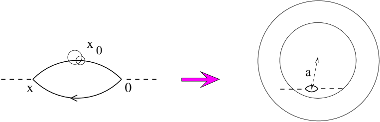
FIG. 5.: Inversion of the polarization operator in the valley background.

so we can use the expansion (26) (in the coordinate space)

$$\langle j_{\mu}(x)j_{\nu}(0)\rangle_{A}~{}\rightarrow~{}-{\sum e_{q}^{2}\over 384\pi^{4}}\Big{[}{2x_{\mu}x_{\nu}+x^{2}\delta_{\mu\nu}\over x^{4}}G^{2}(0)+c\alpha_{s}G^{3}(0)\big{(}2{x_{\mu}x_{\nu}\over x^{2}}-3\delta_{\mu\nu}\ln x^{2}\big{)}+...\Big{]}$$ (40)

and obtain

$$\Pi^{v}(x)\rightarrow$$ (41)

$${\sum e_{q}^{2}\over 192\pi^{4}}\Bigg{[}{\rho^{8}G_{s}^{2}(0)\over y^{4}x_{0}^{4}x^{2}}\Big{\{}1-{4(x_{0}y)^{2}\over x_{0}^{2}y^{2}}\Big{\}}+c\alpha_{s}{\rho^{12}G_{s}^{3}(0)\over y^{6}x_{0}^{6}}\Big{\{}\left(3\ln{\rho^{2}x^{2}\over y^{2}x_{0}^{2}}-1\right){2(x_{0}y)^{2}\over x_{0}^{2}y^{2}}+1\Big{\}}\Bigg{]}$$ (42)

where $G^{s}_{\mu\nu}(0)$ is the field strength of the spherical configuration (38) calculated at at the origin. After the integration over $x$ and $x_{0}$ the first term $\sim G_{s}^{2}$ vanishes and the second gives

$$\int dxe^{iqx}\int dx_{0}{1\over y^{6}x_{0}^{6}}\Big{[}\Big{(}3\ln{x^{2}\over y^{2}x_{0}^{2}}-1\Big{)}{2(x_{0}y)^{2}\over x_{0}^{2}y^{2}}+1\Big{]}={\pi^{4}\over 32}(6\ln\pi+3C-2)q^{4}\ln^{2}q^{2}\,,$$ (43)

leading to

$$\int dxdx_{0}e^{iqx}\Pi^{v}(x)=c^{\prime}\alpha_{s}(q){\sum e_{q}^{2}\over 64}\rho^{6}{\cal G}(z,R^{2}/\rho^{2})q^{4}\ln^{2}q^{2}$$ (44)

where

$${\cal G}(z,R^{2}/\rho^{2})=\rho^{6}G_{s}^{3}(0)$$ (45)

is a dimensionless non-singular function of $z$ and $R^{2}/\rho^{2}$ (the explicit expression can be easily found from Eq. (38)). The argument of $\alpha_{s}$ in Eq. (42) is determined by the characteristic momenta in the loop with one extra gluon in the valley background. After inversion, the characteristic distances in the loop diagram determining the coefficient in front of $G_{s}^{3}$ are $\sim\rho^{2}\sqrt{{x^{2}\over x_{0}^{2}y^{2}}}$ which means that before inversion the characteristic momenta in the loop were $\sim q$ (in the integral (46) $x^{2}\sim x_{0}^{2}\sim y^{2}\sim q^{-2}$).

Performing the integration over $R$ we obtain the analog of the Eq. (33) for the UV renormalon

$$D(q^{2})\simeq q^{2}\alpha_{s}(q)\int_{0}^{1}\!dt\!\int_{0}^{\infty}\!d\rho\rho(\ln q^{2}\rho^{2})^{2}e^{-{4\pi\over\alpha_{s}(\rho)}t}\tilde{\Psi}(t)$$ (46)

leading to

$$D(t)\simeq\tilde{\Psi}(t)q^{2}\!\int_{0}^{\infty}\!\!d\rho^{2}(q^{2}\rho^{2})^{bt}(\ln q^{2}\rho^{2})\left(\alpha_{s}(\rho)/\alpha_{s}(q)\right)^{{2b^{\prime}t\over b}}.$$ (47)

Note that extra $\alpha_{s}(q)$ in Eq. (46) is compensated by one power of $\ln q^{2}\rho^{2}$. The integral over $\rho$ diverges at $t=-{1\over b}$ which is the position of the first UV renormalon. At the one-loop level this renormalon is a double pole $(1+t/b)^{-2}$, same as in the perturbative analysis [4]). Subsequent terms in the expansion (26) correspond to the UV renormalons located at $t=-{2\over b},-{3\over b},-{4\over b}...$ . It should be mentioned that the Eq. (47) cannot reproduce the strength of the first UV renormalon at the two-loop level[14]. The reason is that in Eqs. (26), (42) we have neglected the anomalous dimensions of the operators $\sim(\alpha_{s}(q)/\alpha_{s}(\rho))^{\gamma\over b}$. Such factors can change the strength of the singularity. For the IR renormalon this does not matter since the operator $G^{2}$ is renorm-invariant ($\gamma=0$) and for the subsequent renormalons we can easily correct our results by corresponding $\gamma$’s. Unfortunately, for the UV renormalons we do not know how to use the conformal invariance with the anomalous dimensions included.

VI Conclusions

We have demonstrated that the integration along the dilatation modes in the functional space near the $I\bar{I}$ configuration leads to the renormalon singularities in the Borel plane. It is very important to note that we actually never use the explicit form of the valley configuration. What we have really used are the three facts: (I) conformal anomaly $\Rightarrow$ the fact that the rescaling of the vacuum fluctuation with an action S by a factor $\lambda$ multiplies the determinant by $\lambda^{bS/8\pi^{2}}$ leading to the formula (16), (II) the expansion of the polarization operator (26) in slow varying fields, and (III) the conformal invariance of QCD at the tree level (for the UV renormalon we wrote down the small-size configuration as an inversion of a large-scale vacuum fluctuation). All of these properties hold true for an arbitrary vacuum fluctuation so we could take an arbitrary valley and arrive at the same results Eq. (34) and Eq. (47) . It means that our result about the renormalon singularity coming from the dilatation mode in the functional space is general.

The form of the polarization operator in a valley background suggests the following parametrization of Adler’ function as a double integral in $S$ and $\rho$

$$D(\alpha_{s}(q))=\int_{0}^{\infty}dt\int{d\rho^{2}\over\rho^{2}}d(q^{2}\rho^{2},t)e^{-{4\pi\over\alpha_{s}(\rho)}t}$$ (48)

where

$$d(q^{2}\rho^{2},t)\sim(q^{2}\rho^{2})^{-2}~{}~{}{\rm at}~{}~{}\rho\rightarrow\infty,~{}~{}~{}~{}~{}~{}~{}~{}~{}~{}~{}~{}d(q^{2}\rho^{2},t)\sim(q^{2}\rho^{2})~{}~{}{\rm at}~{}~{}\rho\rightarrow 0$$ (49)

The function $d(q^{2}\rho^{2},t)$ contains only instanton-induced singularities in $t$ whereas the IR and UV renormalons come from the divergence of the integral (48) at large or small $\rho$, respectively. If we “switch off” the running coupling constant (e.g consider the conformal theory without $\beta$-function) the representation of Adler’s function takes the form

$$D^{\rm conf}(\alpha_{s})=\int_{0}^{\infty}dte^{-{4\pi\over\alpha_{s}}t}D^{\rm conf}(t)$$ (50)

where $D^{\rm conf}(t)=\int{d\rho^{2}\over\rho^{2}}d(q^{2}\rho^{2},t)$ (the integral over $\rho$ converges due to Eq. (49)). In real QCD the function $D^{\rm conf}(\alpha_{s})$ defines the “conformal expansion” of the Adler’s function with the coefficients coming from the “skeleton diagrams” in terms of usual perturbation theory[16].

As we mentioned above, our analysis of renormalons is applicable to the “off-shell” processes which can be related to the Euclidean correlation functions of two (or more) currents. One of possible directions of the future work would be to generalize these ideas to the renormalons in the ”on-shell” (Minkowskian) processes intensively discussed in the current literature (see discussion in ref. [4]).

Finally, we note that our method gives same results as the conventional approach - namely position and strength of the renormalon singularity, but not the coefficient in front of it. The coefficient in front of the first IR renormalon is expremely important since it determines the numerical value of asymptotics of perturbative series for $R_{e^{+}e^{-}\rightarrow{\rm hadrons}}$. In principle, for a given valley it is possible to calculate this coefficient in the first order in coupling constant $g^{2}(\rho)$ since it is given by a product of the determinants in the valley background, which can at least be computed numerically. However, the fact that an extra $g^{2}(\rho)$ does not change the position and/or character of the singularity means that all terms in the perturbative series in $g^{2}(\rho)$ contribute on equal footing. This is closely related to the fact that the choice of the valley is not unique: after the change of the valley, the new leading-order coefficient, which comes from the determinants in the background of a new configuration, is given by an infinite perturbative series in $g^{2}(\rho)$ (coming from quantum corrections) in terms of the original valley. As a result, finding the coefficient in front of the leading IR singularity would require the integration over all possible valleys. This study is in progress.

Acknowledgements.

One of us (I.B.) is grateful to V.M. Braun, S.J. Brodsky, R.L. Jaffe, A.H. Mueller, and E.V. Shuryak for valuable discussions. This work was supported by the US Department of Energy under contracts DE-AC05-84ER40150 and DE-FG02-97ER41028.

VII Appendix

We will prove that rescaling of the arbitrary configuration by factor $\lambda$ (so that $\rho\rightarrow\lambda\rho$) leads at the one-loop level to multiplication of the determinant by a factor of

$$\lambda^{bS/8\pi^{2}}$$ (51)

where $S$ is the action of this configuration. Let us demonstrate it for the determinant of the Dirac operator in the background of a field $A_{\mu}(x;\rho)$ characterized by the size $\rho$. We will prove that

$$\sqrt{\det\not\!\tilde{P}^{2}}=\sqrt{\det\not\!P^{2}}~{}\lambda^{{S\over 12\pi^{2}}}$$ (52)

where $P_{\mu}=i\partial_{\mu}+A_{\mu}(x)$ is the operator of the covariant momentum for our configuration and $\tilde{P}_{\mu}=i\partial_{\mu}+\tilde{A}_{\mu}(x)$ is the covariant momentum in the background of the stretched configuration $\tilde{A}_{\mu}(x)=A_{\mu}(x;\lambda\rho)=\lambda^{-1}A_{\mu}(\lambda^{-1}x;\rho)$. Using Schwinger’s notations we can write down

$$\ln\det\not\!\tilde{P}^{2}=-\int_{0}^{\infty}{ds\over s}\int d^{4}x{\rm Tr}(x|e^{-s\not\tilde{P}^{2}}|x)$$ (53)

where $|x)$ are the eigenstates of the coordinate operator normalized according to $(x|y)=\delta^{(4)}(x-y)$. For the Dirac operator, the integral in Eq. (53) diverges so we will assume a cutoff $s>\epsilon$ and take $\epsilon\rightarrow 0$ in the final results. After change of variables $x\rightarrow\lambda^{-1}x$, the integral in the r.h.s. of Eq. (53) reduces to

$$\ln\det\not\!\tilde{P}^{2}=-\int_{0}^{\infty}{ds\over s}\int d^{4}x{\rm Tr}(x|e^{-s\lambda^{-2}\not{P}^{2}}|x)$$ (54)

so

$$\ln\det\not\!\tilde{P}^{2}-\ln\det\not\!P^{2}=$$ (55)

$$\int_{0}^{\infty}{ds\over s}\int d^{4}x{\rm Tr}(x|e^{-s\lambda^{-2}\not{P}^{2}}-e^{-s\not{P}^{2}}|x)=-\lim_{\epsilon\rightarrow 0}\int^{\epsilon}_{\lambda^{-2}\epsilon}{ds\over s}\int d^{4}x{\rm Tr}(x|e^{-s\not{P}^{2}}|x)$$ (56)

Using the well-known result for the DeWitt-Seeley coefficients for the Dirac operator (see e.g. [18])

$${\rm Tr}(x|e^{-s\not{P}^{2}}|x)={3\over 4\pi^{2}s^{2}}+{1\over 48\pi^{2}}G^{a}_{\mu\nu}(x)G^{a}_{\mu\nu}(x),$$ (57)

we obtain

$$\ln\det\not\!\tilde{P}^{2}=\ln\det\not\!P^{2}-{\ln\lambda\over 24\pi^{2}}\int d^{4}xG^{va}_{\mu\nu}G^{va}_{\mu\nu}$$ (58)

which corresponds to the Eq. (52). In the case of $n_{f}$ quark flavors, the coefficient ${1\over 12\pi^{2}}$ in r.h.s. of Eq. (52) will be multiplied by $n_{f}$ leading to the factor $\lambda^{-{2\over 3}n_{f}S/8\pi^{2}}$. This factor is easily recognized as a quark part of the one-loop coefficient $b$ for Gell-Mann-Low $\beta$-function in Eq. (51). Similarly, the rescaling of the gluon (and ghost) determinants reproduces $11$ - the gluon part of the one-loop coefficient $b$ in Eq. (51). Thus we have shown that $e^{-{S\over g^{2}}}\rightarrow e^{-{S\over g^{2}(\rho)}}$ with one-loop accuracy. Using the two-loop formulas for the Seeley coefficients one could prove that $e^{-{S\over g^{2}(\rho)}}$ reproduces at the two-loop level and demonstrate that $g^{2}\rightarrow g^{2}(\rho)$ in the pre-exponential factor $g^{-17}$ as well (as it follows from the renormalizability of the theory).

REFERENCES

- [1] Large order behavior of perturbation theory, ed. J.C. Le Guillou and J. Zinn-Justin, North-Holland, Amsterdam (1990).
- [2] L.N. Lipatov, Sov. Phys. JETP 44 (1976) 1055; 45 (1977) 216.
- [3] G ’t Hooft, in The why’s of Subnuclear Physics (Erice, 1977), ed A. Zichichi (Plenum, New York, 1977)
- [4] M.Beneke, Phys. Reports 317 (1999) 1.
- [5] E.B. Bogomolny and V.A. Fateyev, Phys. Lett. 71B (1977) 93.
- [6] I. Balitsky and A.V. Yung, Phys. Lett. 168B (1986) 113; Nucl. Phys.B 274 (1986) 475
-
[7]
M.Beneke and V.M.Braun,
Nucl. Phys.B 426 (1994)301;
I.I. Bigi, M.A. Shifman, N.G. Uraltsev, and A.I. Vainshtein, Phys. Rev.D 50 (1994) 2234. - [8] A.V. Yung, Nucl. Phys.B 297 (1988) 47.
- [9] I. Balitsky and A. Schafer, Nucl. Phys.B 404 (1993) 639.
- [10] I. Balitsky, Phys. Lett. 273B (1991) 282.
- [11] M.A. Shifman, A.I. Vainshtein, and V.I. Zakharov, Nucl. Phys.B 147 (1979) 1.
- [12] A.H. Mueller, Nucl. Phys.B 250 (1985)327.
- [13] M.S. Dubovikov and A.V. Smilga, Nucl. Phys.B 185 (1981)109, W. Hubschmid and S. Mallik, Nucl. Phys.B 207 (1982) 29.
- [14] M. Beneke, V.M.Braun, and N. Kivel, Phys. Lett. 457B (1999)147.
- [15] M.N. Chernodub, M.I. Polikarpov, and V.I. Zakharov, Phys. Lett. 404B (1997)315.
-
[16]
S.J. Brodsky, E. Gardi, G. Grunberg, and J. Rathsman,
Conformal expansion and renormalons, SLAC-PUB-8362, CPTH-S-746-1099,
LPT-ORSAY-00-09, CERN-TH-2000-032, Feb 2000.
e-Print Archive: hep-ph/0002065 - [17] A.S. Schwarz, Quantum field theory and topology, Springer Verlag, 1993.
- [18] B.S. DeWitt, Dynamical theory of groups and fields, Gordon and Breach, New York, 1965