Non-factorizable effects in the $B-\bar{B}$ mixing

Abstract

We analyse the corrections to factorization for the $B-\bar{B}$ mixing amplitude assuming that non-factorizable soft gluon exchanges can be described by the local gluon condensate. Within this approximation the $\langle\alpha_{s}GG\rangle$-correction to the mixing amplitude can be expressed through the $B$-meson transition form factors at zero momentum transfer. The correction is negative independent of the particular values of the form factors.

As a next step, we study these form factors making use of the relativistic dispersion approach based on the constituent quark picture. We obtain spectral representations for the form factors in terms of the $B$-meson soft wave function and the propagator of the color-octet $b\bar{q}$ system. The $B$-meson wave function has been determined previously from weak exclusive $B$ decays, so the main uncertainty in our estimates comes from the unknown details of the propagator in the nonperturbative region. We obtain $\Delta B_{B_{d}}(m_{b})=-0.06\pm 0.035$ and $\Delta B_{B_{s}}(m_{b})=-0.05\pm 0.03$.

I Introduction

The study of the oscillations in the system of neutral $B$ mesons provides important information on the pattern of the CP violation in the Standard model and its extentions (a detailed discussion can be found in [1]). The main uncertainty in the theoretical description of the process arises from the nonperturbative long-distance contributions to the mixing amplitude. In the $B-\bar{B}$ mixing there are two kinds of such contributions: first, effects related to the presence of the $B$-mesons in the initial and final states, and, second, corrections to the weak 4-quark amplitude due to the soft gluon exchanges between quarks of the initial $B$ and the final $\bar{B}$ meson. By neglecting the second contribution the amplitude factorizes. In this case all nonperturbative effects connected with the meson formation are reduced to only one quantity - the leptonic decay constant $f_{B}$.

Soft-gluon corrections to the weak 4-quark amplitude give rise to non-factorizable contributions, such that the influence of the $B$-meson structure is no longer described by the decay constant only. The understanding of the actual size of the non-factorizable effects and their adequate description in the heavy quark systems is an important and challenging task.

The theoretical analysis of $B-\bar{B}$ mixing was first performed within the QCD sum rules [2, 3, 4] and later using lattice QCD, see [5, 6] and refs therein. The results from the sum rules are in all cases well compatible with factorization (vacuum saturation), within rather large errors. Recent lattice analyses definitely reported negative non-factorizable effects, around 5-10% for the central values at the scale $\mu\simeq m_{b}$. Still, the errors of the calculations have a similar size. Results from these approaches are shown in Table I.

TABLE I.: Comparison of results from various approaches

Ref.	$B_{B_{d}}(m_{b})$	$B_{B_{s}}(m_{b})$	$\hat{B}_{B_{d}}$	$\hat{B}_{B_{s}}/\hat{B}_{B_{d}}$
SR[2, 3]	$1.0\pm 0.15$
SR [4]	$0.95\pm 0.1$
Lat [5]	0.92(4)${}^{+3}_{-0}$	0.91(2)${}^{+3}_{-0}$	1.41(6)${}^{+5}_{-0}$	0.98(3)
Lat [6]	0.93(8)	0.92(6)	1.38(11)	0.98(5)
This work	$0.94\pm 0.035$	$0.95\pm 0.03$	$1.4\pm 0.05$	$1.01\pm 0.01$

In this letter we analyse corrections to factorization in the $B-\bar{B}$ mixing due to soft gluon exchanges in the leading $\alpha_{s}$-order, assuming that the main effect of such exchanges can be described by the local gluon condensate [7]. We show that within this approximation the parameter $\Delta B_{B}$ which describes correction to factorization, is determined by the meson transition form factors at zero momentum transfer. It is important that $\Delta B_{B}$ turns out to be negative, independently of the particular values of these form factors.

As a next step we calculate the relevant form factors. To this end we make use of the relativistic dispersion approach based on the constituent quark picture [8]. We obtain spectral representations for the form factors in terms of the $B$-meson wave function and the propagator of the color-octet $b\bar{q}$-system.

Parameters of the model, such as the quark masses and the wave functions, are known from the analysis of the weak $B$-meson form factors [9, 10] within the same dispersion approach. For numerical estimates we also need the propagator of the color-octet $q\bar{b}$-system in the nonperturbative region, so we discuss the possible form of this propagator. The lack of reliable information about its details in the nonperturbative region leads to the main uncertainties in our numerical estimates.

The paper is organised as follows: The next Section presents basic formulas for the $B-\bar{B}$ mixing. In Section III we calculate the non-factorizable contribution to the mixing amplitude induced by the local gluon condensate and show that the correction is negative. In Section IV we calculate the $B$-meson transition form factors within the dispersion approach. Section V gives numerical estimates.

II Effective Hamiltonian and the structure of the amplitude

The effective Hamiltonian which summarizes the perturbative QCD corrections for the $B^{0}-\bar{B}^{0}$ mixing has the following form [11]

$$H^{\Delta B=2}_{eff}=\frac{G^{2}_{F}\,M^{2}_{W}}{\sqrt{2}}\,\left(V^{*}_{tb}V_{td}\right)^{2}\,C(\mu)\,\left(\bar{b}O_{\sigma}d\right)\left(\bar{b}O_{\sigma}d\right)+h.c.$$ (1)

where $G_{F}$ is the Fermi constant, $O_{\sigma}=\gamma_{\sigma}(1-\gamma_{5})$, $\gamma^{5}=i\gamma^{0}\gamma^{1}\gamma^{2}\gamma^{3}$. The parameter $\mu$ stands for the renormalization scale which separates the hard region taken into account perturbatively and the soft region. The Wilson coefficient $C(\mu)$ includes perturbative corrections above the scale $\mu$. The explicit expression for $C(\mu)$ can be taken from [11]. The soft contributions are contained in the $B$-meson matrix elements of the operators in the effective Hamiltonian

$$A=\left<\bar{B}^{0}\left|\left(\bar{b}O_{\sigma}d\right)\left(\bar{b}O_{\sigma}d\right)\right|B^{0}\right>.$$ (2)

The diagrammatic representation for the amplitude $A$ of Eq. (2) is shown in Fig 1.

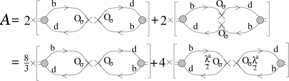
FIG. 1.: Different representations for the $B^{0}-\bar{B}^{0}$ mixing amplitude. The enclosed quark lines show the order of contraction of the spinorial indices. The circles stand for the initial (final) $B$ ($\bar{B}$) meson. The second line is obtained from the first line by performing the combined color and spinorial Fierz rearrangements.

Using the language of the hadronic intermediate states one finds that the contribution of the hadronic vacuum to this amplitude gives

$$\left<\bar{B}^{0}|H^{\Delta B=2}_{eff}|B^{0}\right>=\frac{8}{3}\,\frac{G^{2}_{F}\,M^{2}_{W}\,M^{2}_{B}}{\sqrt{2}}\,(V^{*}_{tb}V_{td})^{2}\,C(\mu)\,f^{2}_{B},$$ (3)

with $f_{B}$ the leptonic decay constant of the $B$ meson defined according to the relation $\left<0|\bar{b}\gamma_{\mu}\gamma_{5}d|B(p)\right>=i\,f_{B}\,p_{\mu}$. It is convenient to parametrize the full amplitude as follows

$$\left<\bar{B}^{0}|H^{\Delta B=2}_{eff}|B^{0}\right>=\frac{8}{3}\,\frac{G^{2}_{F}\,M^{2}_{W}\,M^{2}_{B}}{\sqrt{2}}\,(V^{*}_{tb}V_{td})^{2}\,C(\mu)\,f^{2}_{B}\,B_{B},$$ (4)

such that the quantity $B_{B}-1\equiv\Delta B_{B}$ measures contributions of the non-vacuum intermediate hadronic states.

Using the language of quarks and gluons, the corrections to the amplitude of Fig. 1 due to soft gluon exchanges are obtained by inserting the (soft) gluons between the quark lines in Fig 1. Soft gluon exchanges between the quarks of the same loop lead to the $\alpha_{s}$-corrections either to the meson vertices or to the quark propagators. They only contribute to the leptonic decay constant $f_{B}$ but do not lead to non-factorizable effects.

The non-factorizable effects originate from the soft gluon exchanges between quarks of different loops. To lowest $\alpha_{s}$-order these effects are described by the 4 diagrams shown in Fig. 2.

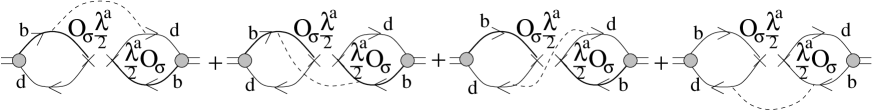
FIG. 2.: Soft-gluon exchanges leading to the non-factorizable effects.

We assume that the main effect of the soft gluon exchange can be described by the local gluon condensate. In the next section we demonstrate that in this approximation the $\left<\alpha_{s}GG\right>$-correction to the factorization is negative.

III $\Delta B$ in terms of the local gluon condensate

Let us consider the exchange of a soft gluon between different quark loops assuming the dominance of the local gluon condensate [7]. In this case a typical graph of Fig 2 describing the soft-gluon contribution is reduced to the product of the three-point diagrams as shown in Fig 3.

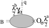
FIG. 3.: Diagrams for $T^{ab(l)}_{\sigma\alpha}(p,q)$ (a) and $T^{ab(r)}_{\sigma\alpha}(p,q)$ (b).

The corresponding amplitude has the form

$$A^{(1)}=g^{2}\int dqdq^{\prime}T^{ab(l)}_{\sigma\alpha}(p,q)T^{ab^{\prime}(r)}_{\sigma\alpha^{\prime}}(p,q)\frac{dx}{(2\pi)^{4}}\frac{dx^{\prime}}{(2\pi)^{4}}{\rm e}^{-iqx+iq^{\prime}x^{\prime}}\langle A^{b}_{\alpha}(x)A^{b^{\prime}}_{\alpha^{\prime}}(x^{\prime})\rangle,$$ (5)

where $T^{ab(l)}_{\sigma\alpha}(p,q)$ with the superscript $l$ stands for the amplitude of Fig 3a with the $B$ in the initial state, and $T^{ab^{\prime}(r)}_{\sigma\alpha^{\prime}}(p,q^{\prime})$ with the superscript $r$ for the amplitude of Fig 3b with the $\bar{B}$ in the final state.

It is convenient to use the fixed-point gauge $x_{\mu}A^{b}_{\mu}(x)=0$ [12]. In this case the gluon potential reads

$$A^{b}_{\alpha}(x)=\frac{1}{2}x_{\beta}G^{b}_{\alpha\beta}+...,$$ (6)

where dots stand for terms with higher order derivatives. The average over the hadronic vacuum is performed according to the relation

$$\langle G^{b}_{\alpha\beta}G^{b^{\prime}}_{\alpha^{\prime}\beta^{\prime}}\rangle=\frac{\delta^{bb^{\prime}}}{96}(g_{\alpha\alpha^{\prime}}g_{\beta\beta^{\prime}}-g_{\alpha\beta^{\prime}}g_{\alpha^{\prime}\beta})\langle GG\rangle,$$ (7)

with $\delta^{aa}=N_{c}^{2}-1$. Here $\langle GG\rangle$ is the positive-valued gluon condensate $\langle\frac{\alpha_{s}}{\pi}GG\rangle=0.012\;{\rm GeV}^{4}$ [7].

The amplitude of Fig 3 then takes the form

$$A^{(1)} = \frac{g^{2}}{4}\int dqdq^{\prime}T^{ab(l)}_{\sigma\alpha}(p,q)\frac{\partial}{\partial q_{\beta}}\delta(q)T^{ab^{\prime}(r)}_{\sigma\alpha^{\prime}}(p,q^{\prime})\frac{\partial}{\partial q^{\prime}_{\beta^{\prime}}}\delta(q^{\prime})\langle G^{b}_{\alpha\beta}G^{b^{\prime}}_{\alpha^{\prime}\beta^{\prime}}\rangle$$ (8)

$$= \frac{g^{2}}{4}\langle G^{b}_{\alpha\beta}G^{b^{\prime}}_{\alpha^{\prime}\beta^{\prime}}\rangle\frac{\delta^{ab}}{2\sqrt{N_{c}}}T^{(l)}_{\sigma\alpha,\beta}(p)\frac{\delta^{ab^{\prime}}}{2\sqrt{N_{c}}}T^{(r)}_{\sigma\alpha^{\prime},\beta^{\prime}}(p),$$ (9)

where we have denoted

$$\frac{\partial}{\partial q_{\beta}}T^{ab(l,r)}_{\sigma\alpha}(p,q)|_{q=0}\equiv\frac{\delta^{ab}}{2\sqrt{N_{c}}}T^{(l,r)}_{\sigma\alpha,\beta}(p).$$ (10)

Notice that only the parts of the amplitudes $T^{(l,r)}$ antisymmetric in indices $\alpha$ and $\beta$ give a nonvanishing contribution. These antisymmetric parts have the following general Lorentz structure:

$$T^{A(l,q)}_{\sigma\alpha,\beta} = 4p^{\nu}\left[f_{1}^{q}\epsilon_{\alpha\beta\sigma\nu}+if_{2}^{q}(g_{\alpha\nu}g_{\beta\sigma}-g_{\beta\nu}g_{\alpha\sigma})\right],$$ (11)

$$T^{A(l,\bar{q})}_{\sigma\alpha,\beta} = 4p^{\nu}\left[f_{1}^{\bar{q}}\epsilon_{\alpha\beta\sigma\nu}+if_{2}^{\bar{q}}(g_{\alpha\nu}g_{\beta\sigma}-g_{\beta\nu}g_{\alpha\sigma})\right],$$ (12)

$$T^{A(r,q)}_{\sigma\alpha,\beta} = T^{A(l,\bar{q})}_{\sigma\alpha,\beta},$$ (13)

$$T^{A(r,\bar{q})}_{\sigma\alpha,\beta} = T^{A(l,q)}_{\sigma\alpha,\beta},$$ (15)

$$f_{1}^{q}=f_{1}^{\bar{q}},\qquad f_{2}^{q}=-f_{2}^{\bar{q}}.$$

The superscript $q(\bar{q})$ in these expressions denotes the flavour of the quark (antiquark) to which the soft external gluon is attached in diagrams of Fig 3. The quantities $f_{1,2}^{q,\bar{q}}$ are real constants. The last three lines in Eq. (11) are the consequence of the $C$-invariance of the strong interaction $S$-matrix. As we discuss in the next section, the constants $f_{1,2}^{q,\bar{q}}$ can be represented as specific $B$-meson transition form factors at zero momentum transfer.

We have to collect now contributions of the four diagrams in Fig 2. For instance, the contribution to the amplitude of the subprocess in which the soft gluons are attached to the $b$ quark in the left loop and the $\bar{b}$ quark in the right loop reads

$$T^{A(l,b)}_{\sigma\alpha;\beta}(p)T^{A(r,\bar{b})}_{\sigma\alpha^{\prime};\beta^{\prime}}(p)(g_{\alpha\alpha^{\prime}}g_{\beta\beta^{\prime}}-g_{\alpha\beta^{\prime}}g_{\alpha^{\prime}\beta})=-192M_{B}^{2}\left((f^{b}_{1})^{2}+(f^{b}_{2})^{2}\right).$$ (16)

Similar expressions are easily obtained for other diagrams using the relations (11). Taking into account the relevant symmetry factors as shown in Fig 1, we finally arrive at the following expressions (we also list the factorizable amplitude in the same normalization)

$$A^{(0)} \simeq \frac{8}{3}M_{B}^{2}f_{B}^{2}$$ (17)

$$A^{(1)} \simeq -8C_{F}M_{B}^{2}\left<\frac{\alpha_{s}}{\pi}GG\right>\pi^{2}\left[(f_{1}^{b}+f_{1}^{d})^{2}+(f_{2}^{b}-f_{2}^{d})^{2}\right],$$ (18)

with the color factor $C_{F}=\frac{N_{c}^{2}-1}{4N_{c}}$. Finally, for $\Delta B_{B}$ we find the expression

$$\Delta B_{B}(\mu)=-\frac{\left<\frac{\alpha_{s}}{\pi}GG\right>}{f_{B}^{2}}2\pi^{2}\left[\left(f_{1}^{b}+f_{1}^{d}\right)^{2}+\left(f_{2}^{b}-f_{2}^{d}\right)^{2}\right].$$ (19)

Obviously, the correction to the factorizable amplitude due to the local gluon condensate is negative. This agrees with all numerical results for $\Delta B$. Notice that the constants $f_{1}$ and $f_{2}$ depend on the renormalization scale $\mu$.

IV Form factors in the dispersion approach

We now proceed to the calcuation of the form factors $f_{1}$ and $f_{2}$. To this end we make use of the relativistic dispersion approach based on the constituent quark picture. Within this approach all observables are given by the spectral representations in terms of the soft wave function of the participating mesons.

We start with the amplitude $T^{(l)ab}_{\sigma\alpha}(p,q)$. It is diaginal in color indices, so we write $T^{(l)ab}_{\sigma\alpha}(p,q)=\frac{\delta^{ab}}{\sqrt{N_{c}}}T^{(l)}_{\sigma\alpha}(p,q)$. The triangle diagram for $T^{(l)}_{\sigma\alpha}(p,q)$ is shown in Fig. 4a. Throughout this section we shall omit the superscript $l$. The quark structure of the $B$-meson is described by the vertex $i\bar{q}_{1}\gamma_{5}q_{2}G(s)/\sqrt{N_{c}}$, where $s$ is the invariant mass of the $q_{1}\bar{q}_{2}$ pair [8]. One should set $m_{1}=m_{b}$, $m_{2}=m_{d}$ for the calculation of $f^{(b)}$, and $m_{1}=m_{d}$, $m_{2}=m_{b}$ for $f^{(d)}$.

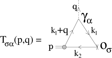
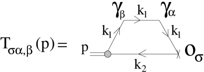
FIG. 4.: Diagrams for $T_{\sigma\alpha}(p,q)$ (a) and $T_{\sigma\alpha,\beta}(p)=\frac{\partial}{\partial q^{\beta}}T_{\sigma\alpha}(p,q)|_{q=0}$ (b).

We need to calculate $T_{\sigma\alpha,\beta}(p)=\frac{\partial}{\partial q^{\beta}}T_{\sigma\alpha}(p,q)|_{q=0}$ (10). For the $T_{\sigma\alpha}(p,q)$ shown in Fig 4a, its derivative $T_{\sigma\alpha,\beta}(p)$ is given by the diagram in Fig 4b. The trace corresponding to the Feynman diagram of Fig 4b reads:

$$S_{\sigma\alpha;\beta}={\rm Sp}\left[i\gamma_{5}(m_{2}-\hat{k}_{2})O_{\sigma}(m_{1}+\hat{k}_{1})\gamma_{\alpha}(m_{1}+\hat{k}_{1})\gamma_{\beta}(m_{1}+\hat{k}_{1})\right],$$ (20)

where $O_{\sigma}=\gamma_{\sigma}(1-\gamma_{5})$. Since this expression is further multiplied by $G_{\alpha\beta}$, only its antisymmetric part in $\alpha$ and $\beta$ is necessary. The latter reads

$$S^{A}_{\sigma\alpha;\beta} = (m_{1}^{2}-k_{1}^{2}){\rm Sp}\left(i\gamma_{5}(m_{2}-\hat{k}_{2})\gamma_{\sigma}(1-\gamma_{5})\gamma_{\beta}(m_{1}-\hat{k}_{1})\right)$$ (21)

$$= (m_{1}^{2}-k_{1}^{2})\left[4\epsilon_{\beta\alpha\sigma\nu}(m_{2}k_{1}^{\nu}+m_{1}k_{2}^{\nu})+4im_{1}k_{2}^{\nu}(g_{\alpha\sigma}g_{\beta\nu}-g_{\beta\sigma}g_{\alpha\nu})\right].$$ (22)

The corresponding expression for the Feynman amplitude takes the form

$$T^{A}_{\sigma\alpha;\beta}(p) = \frac{1}{(2\pi)^{4}i}\int dk_{1}dk_{2}\delta(p-k_{1}-k_{2})\frac{-1}{(m_{1}^{2}-k_{1}^{2})^{2}(m_{2}^{2}-k_{2}^{2})}$$ (24)

$$\times\left[4\epsilon_{\beta\alpha\sigma\nu}(m_{2}k_{1}^{\nu}+m_{1}k_{2}^{\nu})+4im_{1}k_{2}^{\nu}(g_{\alpha\sigma}g_{\beta\nu}-g_{\beta\sigma}g_{\alpha\nu})\right].$$

We define $f_{v}$ and $f_{s}$ by the relations

$$\frac{1}{(2\pi)^{4}i}\int dk_{1}dk_{2}\delta(p-k_{1}-k_{2})\frac{k_{1}^{\nu}}{(m_{1}^{2}-k_{1}^{2})^{2}(m_{2}^{2}-k_{2}^{2})} = p^{\nu}f_{v}(p^{2}),$$ (25)

$$\frac{1}{(2\pi)^{4}i}\int dk_{1}dk_{2}\delta(p-k_{1}-k_{2})\frac{1}{(m_{1}^{2}-k_{1}^{2})^{2}(m_{2}^{2}-k_{2}^{2})} = f_{s}(p^{2}).$$ (26)

After the $k$-integration in Eq. (24) one recovers the structure of the amplitude from Eq. (11)

$$T^{A}_{\sigma\alpha;\beta}(p)=-4p^{\nu}\left[f_{1}\;\epsilon_{\beta\alpha\sigma\nu}+if_{2}\;(g_{\alpha\sigma}g_{\beta\nu}-g_{\beta\sigma}g_{\alpha\nu})\right],$$ (27)

with

$$f_{1} = (m_{2}-m_{1})f_{v}+m_{1}f_{s},$$ (28)

$$f_{2} = m_{1}(f_{s}-f_{v}).$$ (29)

Let us obtain now spectral representations for the form factors $f^{F}_{v}$ and $f^{F}_{s}$. We first notice that the expressions (25) correspond to the triangle Feynman diagram at zero momentum transfer $q=0$. This condition means that both $q^{2}=0$ and $p^{2}=p^{\prime 2}$, where $p^{\prime}=p-q$, so we can write $f^{F}_{i}(p^{2})=f^{F}_{i}(q^{2}=0,p^{2},p^{\prime 2}=p^{2})$, with $i=v,s$.

It is convenient to start with the case $q^{2}\neq 0$ and $p^{2}\neq p^{\prime 2}$. Then the form factors $f_{i}$ can be written in the form of the double spectral representation [8]:

$$f^{F}_{i}(q^{2},p^{2},p^{\prime 2})=\int\frac{ds}{s-p^{2}}\frac{ds^{\prime}}{s^{\prime}-p^{\prime 2}}\Delta_{i}(s,s^{\prime},q^{2}),$$ (30)

where the double spectral density $\Delta_{i}$ can be calculated for any of the form factors from the Feynman integral.

As the next step, we set $q^{2}=0$, but still treat $p^{2}$ and $p^{\prime 2}$ as independent variables. In this case the double spectral representations of the form (30) simplify to the following single spectral representations

$$f^{F}_{s}(p^{2},p^{\prime 2}) = \frac{1}{16\pi^{2}}\int ds\frac{1}{s-p^{2}}\frac{1}{s-p^{\prime 2}}\log\left(\frac{s+m_{1}^{2}-m_{2}^{2}+\lambda^{1/2}(s,m_{1}^{2},m_{2}^{2})}{s+m_{1}^{2}-m_{2}^{2}-\lambda^{1/2}(s,m_{1}^{2},m_{2}^{2})}\right),$$ (31)

$$f^{F}_{v}(p^{2},p^{\prime 2}) = \frac{1}{16\pi^{2}}\int ds\frac{1}{s-p^{2}}\frac{1}{s-p^{\prime 2}}\frac{\lambda^{1/2}(s,m_{1}^{2},m_{2}^{2})}{s}.$$ (32)

The representations for the form factors in the form (32) are valid however only in the region of $p^{2}$ and $p^{\prime 2}$ (far) below the threshold. The reason for that is the following: the representations (30) and (32) are based on the Feynman form of the quark propagators. This form is however valid only for highly virtual particles, while in the soft region it is strongly distorted by nonperturbative effects. In particular, the pole at $k^{2}=m^{2}$ in the propagator of a color object, like quark and gluon, is absent. Recently, this was confirmed in a lattice study of the gluon propagator [13].

The modification of the quark propagator in the soft region leads to the change of the spectral representation for the form factors in the region of $p^{2}$ and $p^{\prime 2}$ near and above the $b\bar{q}$ threshold.

Notice that the quantities $1/(s-p^{2})$ and $1/(s^{\prime}-p^{\prime 2})$ in Eq. (30) are the propagators of the initial and final $b\bar{q}$ states with virtualities $s$ and $s^{\prime}$, and the squared masses $p^{2}$ and $p^{\prime 2}$, respectively. The nonperturbative effects which modify the quark and gluon propagators in the soft region, modify the propagators of the $b\bar{q}$ states as well.

We know the character of these changes in the $p^{2}$-channel corresponding to the $B$-meson: As discussed in [8], soft interaction of quarks effectively replace the factor $1/(s-M_{B}^{2})$ with a regular $B$-meson soft wave function $\phi_{B}(s)$ in the integrand of (32). The $B$-meson soft wave function is normalized as follows [8]

$$\frac{1}{8\pi^{2}}\int ds\phi_{B}^{2}(s)\frac{\lambda^{1/2}(s,m_{b}^{2},m_{q}^{2})}{2s}(s-(m_{b}-m_{q})^{2})=1.$$ (33)

The leptonic decay constant is given by the expression

$$f_{B}=\frac{\sqrt{N_{c}}(m_{b}+m_{q})}{8\pi^{2}}\int ds\phi_{B}(s)\frac{\lambda^{1/2}(s,m_{b}^{2},m_{q}^{2})}{s}\frac{s-(m_{b}-m_{q})^{2}}{s}.$$ (34)

In the color-octet $p^{\prime 2}$-channel the Feynman propagator $1/(s-p^{\prime 2})$ in Eq (32) is replaced by the propagator $D(s,p^{\prime 2})$ which involves proper modifications in the soft region. We therefore find the following representation for the form factors $f_{i}(p^{\prime 2})\equiv f_{i}(q^{2}=0,p^{2}=M_{B}^{2},p^{\prime 2})$

$$f_{v}(p^{\prime 2}) = \frac{1}{16\pi^{2}}\int ds\phi_{B}(s)D(s,p^{\prime 2})\frac{\lambda^{1/2}(s,m_{1}^{2},m_{2}^{2})}{s},$$ (35)

$$f_{s}(p^{\prime 2}) = \frac{1}{16\pi^{2}}\int ds\phi_{B}(s)D(s,p^{\prime 2})\log\left(\frac{s+m_{1}^{2}-m_{2}^{2}+\lambda^{1/2}(s,m_{1}^{2},m_{2}^{2})}{s+m_{1}^{2}-m_{2}^{2}-\lambda^{1/2}(s,m_{1}^{2},m_{2}^{2})}\right).$$ (36)

We know that $D(s,p^{\prime 2})\sim 1/(s-p^{\prime 2})$ at large values of $s-p^{\prime 2}$, and also that $D(s,p^{\prime 2})$ is finite at $s=p^{\prime 2}$. However, we do not know details of $D(s,p^{\prime 2})$ in the soft region. Motivated by the discussion in [14], we assume here that the nonperturbative effects can be described by the following modification of the propagator

$$D(s,p^{\prime 2})=\frac{1}{s-p^{\prime 2}+M_{0}^{2}}$$ (37)

where $M_{0}$ is a mass parameter. In order to guarantee the absence of the pole in $D(s,p^{\prime 2})$ in the heavy quark limit, $M_{0}$ should scale with the heavy quark mass as follows: $M_{0}^{2}=O(\Lambda_{QCD}\,m_{Q})$. So it is convenient to write $M_{0}$ in the form

$$M_{0}^{2}=w\,m_{d}\,m_{b},$$ (38)

where $m_{d}\simeq\Lambda_{QCD}$ is the constituent mass of the light quark, and $w$ is a parameter of order unity.

In the next section we make use of Eqs. (35) and (37) to analyse $f_{v,s}(p^{\prime 2})$ for $B_{d}$ and $B_{s}$ mesons.

V Numerical results.

The parametrization for the $B$-meson wave function and values of the quark masses have been determined from the analysis of the exclusive processes in [9, 10]. The $B$-meson soft wave function can be written in the form

$$\varphi(s)=\frac{\pi}{\sqrt{2}}\frac{\sqrt{s^{2}-(m_{q}^{2}-m_{\bar{q}}^{2})^{2}}}{\sqrt{s-(m_{q}-m_{\bar{q}})^{2}}}\frac{w(k^{2})}{s^{3/4}}$$ (39)

with $k^{2}=\lambda(s,m_{q}^{2},m_{\bar{q}}^{2})/4s$. As found in [10] a simple Gaussian parametrization $w(k^{2})\sim\exp(-k^{2}/2\beta^{2})$ gives a good description of the $B$-meson properties. The numerical parameters of the model from [10] are listed in Table II.

TABLE II.: Constituent quark masses, slope parameters of the Gaussian wave function, and the corresponding calculated leptonic decay constants in GeV from [10].

	$m_{u}$	$m_{s}$	$m_{b}$	$\beta_{B}$	$\beta_{B_{s}}$	$f_{B}$	$f_{B_{s}}$
	0.23	0.35	4.85	0.54	0.56	0.18	0.20

The procedure of Ref. [9, 10] determines the wave function by fitting the lattice data on the weak transition form factors for large momentum transfers at the normalization point $\mu\simeq 5\;$ GeV. Therefore, the $B$-meson soft wave function and the form factors $f_{s,v}(p^{\prime 2})$ at this scale are determined.

Whereas the $B$-meson wave function is known quite well, good information about the details of $D(s,p^{\prime 2})$ is lacking. We therefore use the simple Ansatz (37) for $D(s,p^{\prime 2})$ in the full range of $s$ and $p^{\prime 2}$ and treat $w$ as a free parameter of order unity. We expect that the variation of $w$ in the interval $w=0.5\div 2$ provides reasonable error estimates for the form factors and $\Delta B$. Notice that the value of $\Delta B$ corresponding to $w=1$ agrees favourably with the recent lattice estimates, see Table I. Fig 5 shows the form factor $f_{s}^{(d)}$ which gives the main contribution to $\Delta B_{B}$.

FIG. 5.: The form factor $f_{s}{(p^{\prime 2})}$ for the $B_{d}$ meson vs $p^{\prime 2}$. Solid curves are results of the calculation via the Eqs. (35) and (37) for various values of the parameter $w$: upper curve - $w=0.5$, middle curve - $w=1.0$, lower curve - $w=2$. The dash-dotted curve in the region $p^{\prime 2}<(m_{b}+m_{d})^{2}$ corresponds to $w=0$. The vertical dotted line corresponds to $p^{\prime 2}=M_{B}^{2}$.

The calculated form factors are shown in Table III. The relative magnitudes of these form factors can be easily understood taking into account their scaling propertiers in the heavy quark limit: $f_{s}^{(d)}\sim m_{b}^{-1/2}$, $f_{s}^{(b)}\sim m_{b}^{-3/2}$, $f_{v}^{(b)}/f_{s}^{(b)}\sim 1$.

The value of $\Delta B$ is obtained from Eq. (19) taking $\left<\frac{\alpha_{s}}{\pi}GG\right>=0.012\;{\rm GeV}^{4}$ from [7]. Using the Wilson coefficent at the scale $\mu=m_{b}$ we obtain the renorm-invariant factors $\hat{B}_{B_{d}}$ and $\hat{B}_{B_{s}}$ (for definition see [6]) listed in Table I.

TABLE III.: Form factors and $\Delta B_{B_{q}}$ with $q=d$ for $B_{d}$, and $q=s$ for $B_{s}$. The factors $f_{1,2}(p^{\prime 2})$ are calculated at $p^{\prime 2}=M^{2}_{B_{d}}$ for $B_{d}$ and at $p^{\prime 2}=M^{2}_{B_{s}}$ for $B_{s}$. The errors correspond to the interval $w$=0.5$\div$2.

	$B_{d}$	$B_{s}$
$f_{v}^{(b)}=f_{v}^{(q)}$	$9\pm 3\times 10^{-3}$	$8\pm 3\times 10^{-3}$
$f_{s}^{(b)}$	$1.1\pm 0.2\times 10^{-2}$	$9\pm 3\times 10^{-3}$
$f_{s}^{(d)}$	$1.4\pm 0.5\times 10^{-1}$	$1.0\pm 0.4\times 10^{-1}$
$f_{1}^{(b)}$	$7\pm 1.5\times 10^{-3}$	$8\pm 3\times 10^{-3}$
$f_{2}^{(b)}$	$5.5\pm 1.5\times 10^{-3}$	$5.5\pm 2.0\times 10^{-3}$
$f_{1}^{(d)}$	$7.5\pm 2.5\times 10^{-2}$	$7.5\pm 2.5\times 10^{-2}$
$f_{2}^{(d)}$	$3.5\pm 1.0\times 10^{-2}$	$3.0\pm 1.5\times 10^{-2}$
$\Delta B_{B_{q}}$	$-0.06\pm 0.035$	$-0.05\pm 0.03$

Our results are in good agreement with the lattice results, except for a slightly different estimate of the SU(3) violating effects in the $B_{d}-\bar{B}_{d}$ and $B_{s}-\bar{B}_{s}$ cases. This nice agreement gives support to our Ansatz for the description of the nonperturbative effects in the propagator of the color-octet $q\bar{q}$ system.

We would like to notice that taking the Ansatz (37) and (38) for the propagator of the $s\bar{q}$ system and setting $M_{0}^{2}=w\,m_{s}\,m_{\bar{q}}$, with $w\simeq 1$ allows a parameter-free estimate of the $K^{0}-\bar{K}^{0}$ mixing. In this case the result is much more stable with respect to the particular value of $w$ and therefore to the details of the propagator in the nonperturbative region. We obtained this way $\Delta B_{K}(1\;{\rm GeV})=-0.21\pm 0.04$ [15].

VI Conclusion.

We considered corrections to factorization in the $B\bar{B}$ mixing amplitude due to soft-gluon exchanges, assuming that the main effect of such exchanges can be described in terms of the local gluon condensate.

1. It was demonstrated that within this approximation correction of the order $\alpha_{s}\langle GG\rangle$ to the factorization is negative. It can be expressed through the specific $B$-meson transition form factors at zero momentum transfer.

2. A relativistic dispersion approach based on the constituent quark picture has been used to calculate these form factors. Spectral representations for the form factors in terms of the $B$-meson soft wave function and the propagator of the color-octet $q\bar{b}$ system were obtained. The behaviour of this propagator in the nonperturbative region was discussed. The obtained numerical estimates for $\Delta B_{B}$ favourably compare with the recent lattice calculations.

Let us point out that the proposed approach can be extended to the description of more complicated problems. In particular, it can be applied to the analysis of the non-factorizable effects in non-leptonic $B$ decays.

REFERENCES

[1]G. Buchalla, A. Buras and M. Lautenbacher, Rev. Mod. Phys. 68 (1996) 1125;
A. J. Buras and R. Fleischer, in Heavy Flavours II,
World Scientific (1997), eds. A.J. Buras and M. Linder, p. 65, [hep-ph/9704376].
[2] A. Pich, Phys. Lett. B206 (1988)322.
[3] A. A. Ovchinnikov and A. A. Pivovarov, Yad. Fiz. 48 (1988) 189;
Phys. Lett. B207 (1988) 333;
S. Narison and A. A. Pivovarov, Phys. Lett. B327 (1994) 341.
[4] L. J. Reinders and S. Yazaki, Phys. Lett. B212 (1988) 245.
[5]L. Lellouch and C.-J. Lin, Talk given at
Heavy Flavours 8, Southampton, England, 25-29 July 1999,
[hep-ph/9912322].
[6] D. Becirevic et al, preprint hep-lat/0002025.
[7] M. A. Shifman, A. I. Vainshtein, and V. I. Zakharov,
Nucl. Phys. B147 (1979) 385.