August 2000 OUTP–00–34P UFIFT–HEP–00–19
Solar neutrino oscillation from large extra dimensions

Abstract

A plausible explanation for the existence of additional light sterile neutrinos is that they correspond to modulini, fermionic partners of moduli, which propagate in new large dimensions. We discuss the phenomenological implications of such states and show that solar neutrino oscillation is well described by small angle MSW oscillation to the tower of Kaluza Klein states associated with the modulini. In the optimal case the recoil electron energy spectrum agrees precisely with the measured one, in contrast to the single sterile neutrino case which is disfavoured. We also consider how all oscillation phenomena can be explained in a model including bulk neutrino states. In particular, we show that a naturally maximal mixing for atmospheric neutrinos can be easily obtained.

There are several indications of neutrino mass from experiments sensitive to neutrino oscillation. Recent reports by the Super-Kamiokande collaboration [1], indicate that the number of $\nu_{\mu}$ in the atmosphere is reduced, due to neutrino oscillations. These reports seem to be supported by the recent findings of other experiments [2], as well as by previous observations [3]. The data is consistent with $\Delta m_{\nu_{\mu}\nu_{\tau}}^{2}\approx(10^{-2}\;\text{to}\;10^{-3})\;\,\mathrm{eV}^{2}$, $\sin^{2}2\theta_{\mu\tau}\geq 0.8$ while dominant $\nu_{\mu}\rightarrow\nu_{e}$ oscillations are disfavoured by Super-Kamiokande [1] and CHOOZ [4]. Measurement of solar neutrinos suggest matter enhanced oscillations with either a small mixing angle, $\Delta m_{\nu_{e}\nu_{\alpha}}^{2}\approx(3\,\text{--}\,10)\cdot 10^{-6}\,\mathrm{eV}^{2}$, $\sin^{2}2\theta_{e\alpha}\approx(0.2\,\text{--}\,1.3)\cdot 10^{-2}$, or a large mixing angle, $\Delta m_{\nu_{e}\nu_{\alpha}}^{2}\approx(1\,\text{--}\,20)\cdot 10^{-5}\,\mathrm{eV}^{2}$, $\sin^{2}2\theta_{e\alpha}\approx(0.5\,\text{--}\,0.9)$ or vacuum oscillations $\Delta m_{\nu_{e}\nu_{\alpha}}^{2}\approx(0.5\,\text{--}\,1.1)\cdot 10^{-10}\,\mathrm{eV}^{2}$, $\sin^{2}2\theta_{\alpha e}\geq 0.67$, where $\alpha$ is $\mu$ or $\tau$. Recent measurements of the day night asymmetry and the recoil electron energy spectrum disfavour the small angle MSW solution [8]. The collaboration using the Liquid Scintillator Neutrino Detector at Los Alamos (LSND) has reported evidence for the appearance of $\bar{\nu}_{\mu}-\bar{\nu}_{e}$ [9] and ${\nu}_{\mu}-{\nu}_{e}$ oscillations [10]. Interpretation of the LSND data favours the choice $0.2\,\mathrm{eV}^{2}\leq\Delta m^{2}\leq 10\,\mathrm{eV}^{2}$, $0.002\leq\sin^{2}2\theta\leq 0.03$. Note that if neutrinos provide a significant hot dark matter component, then the heavier neutrino(s) should have mass in the range $\sim(1\,\text{--}\,6)\,\mathrm{eV}$, where the precise value depends on the number of neutrinos that have masses of this order of magnitude [11]. Of course, this requirement is not as acute, since there are many alternative ways to reproduce the observed scaling of the density fluctuations in the universe.

If all these indications should prove to be correct there must be more than 3 light neutrino species because explanation of the data requires 3 different mass differences. This immediately raises the question why these states should be anomalously light. In the case of the three doublet neutrinos the underlying SU(2) gauge symmetry guarantees they should remain massless in the Standard Model. However additional sterile neutrinos do not transform under the Standard Model gauge group and thus some additional ingredient is needed to explain their lightness. A plausible explanation has been given recently in the context of theories with large additional space dimensions.

These are models where the Standard Model (SM) fields are confined to three-branes which are localized in a higher-dimensional gravitation-only bulk. Bulk fermions are, therefore, SM singlets and are associated to Kaluza-Klein towers of 4-dimensional sterile neutrinos. In the context of string- or M-theory derived supersymmetric models the superpartners of moduli fields are particularly interesting candidates for light bulk fermions. Perturbatively, these moduli fields as well as their fermionic partners are exactly massless. Masses for the moduli and modulinos are then generated by non-perturbative effects which, at the same time, may also break supersymmetry. This may account for the lightness of the sterile states. As an example relevant to the present paper, one can consider models with a string scale of order $\,\mathrm{TeV}$ and supersymmetry breaking on the observable brane. These supersymmetry breaking effects would be communicated to the bulk with a suppression of one power of the low-energy Planck scale resulting in a scale of order meV. Therefore, in such models, it is reasonable to expect light bulk masses for moduli and modulini of the order meV.

From the experimental point of view, it seems unlikely that a single sterile neutrino is involved in atmospheric neutrino oscillations [1]. Moreover, as we discuss below, large mixing angles between doublet and singlet neutrinos are ruled out by the constraints following from the requirement that a supernova should not be rapidly cooled by sterile neutrino emission. The possibility that (small angle MSW) oscillations into a single sterile neutrino solve the solar neutrino problem also seems to be disfavoured by recent SuperKamiokande results [8]. The SK preliminary analysis also disfavours the standard small mixing angle solution in the active neutrino case, so that only the large mixing angle solution would be left. We will see, however, that oscillations of solar neutrinos into towers of sterile neutrinos are not disfavoured. On the contrary, they fit very well the presently available data. Furthermore the supernova bounds do allow the small mixing angle needed for this mechanism to work. Therefore, the brane-world scenario, besides being a theoretically well-motivated framework, is an experimentally viable sterile neutrino scenario, given the present experimental status. At the same time, it offers a small mixing alternative to the large mixing angle solution.

The connection between large extra-dimensions and neutrino physics has been discussed in [12] and in [13, 14, 15]. In this letter we present an explicit model showing that the presence of a Dirac bulk mass terms can significantly affect the phenomenology of brane-bulk neutrino models and can open up interesting possibilities from the model-building point of view [15]. A general analysis of the impact of different possible mass terms will be given elsewhere [16]. As for solar neutrino oscillations, we will descibe new schemes that include a modified version of the “massless” model in [13]. A detailed fit including the latest SK (1117 days) and GNO data will show the beautiful agreement with experiment. We will then see how a maximal angle for $\nu_{\mu}\leftrightarrow\nu_{\tau}$ atmospheric neutrino oscillations can be naturally generated. The model has also room for $\nu_{e}\leftrightarrow\nu_{\mu}$ oscillations with a ${\Delta m^{2}_{\text{}}}$ larger than the atmospheric one, that can be used to accommodate the LSND signal.

We first briefly describe the model from a 5-dimensional point of view. We will then translate it into a 4-dimensional language and study its phenomenology. We consider an effective 5-dimensional model with an approximate “lepton number” U(1) symmetry. Under this symmetry the SM leptons as well as a set of bulk spinors $\Psi_{I}$, where $I=1,\ldots,N$, carry charge $L=1$. A 6-dimensional explicit example with a similar structure has been described in [15]. In this paper, we consider a 5-dimensional model with the free bulk action given by

$$S_{\text{bulk}}=\int d^{4}x\,dy\,\left(\overline{\Psi}_{I}\gamma^{A}i\partial_{A}\Psi_{I}-\mu_{I}\overline{\Psi}_{I}\Psi_{I}\right)\;.$$ (1)

Here, $x=(x^{0},\ldots,x^{3})$ are the coordinates longitudinal to the brane, $y=x^{4}$ is the transverse coordinate, $\gamma^{A}$, where $A=0\ldots 4$, are the 5-dimensional gamma matrices and $\mu_{I}\geq 0$ are Dirac masses. This action for the bulk fermions is the most general free one compatible with 5-dimensional Lorentz- and U(1)-symmetry up to a field redefinition. Mass terms breaking the Lorentz symmetry can also arise [16] but will not be considered here.

The most naive brane-bulk coupling is that between the standard model invariants $L_{i}H$ and the five-dimensional fermion fields $\Psi_{I}$ (or their conjugates), evaluated at the brane which we locate at $y=0$. This coupling takes the form

$$S_{\text{brane}}=-\int_{y=0}d^{4}x\,\left(\frac{h_{Ii}}{\sqrt{M_{5}}}\overline{\Psi}_{Ii}L_{i}H+\frac{h^{c}_{Ii}}{\sqrt{M_{5}}}\overline{\Psi^{c}}_{Ii}L_{i}H\right)+\text{h.c.}\;.$$ (2)

Here, $L_{i}$, where $i=e,\mu,\tau$, are the three lepton doublets in a basis in the family space that diagonalizes the charged lepton mass matrix. Furthermore, $H$ is the relevant Higgs field, $\Psi^{c}$ is the charged-conjugated fermion and $M_{5}$ is the effective 5-dimensional Planck scale. Note that the coupling $h$ respects the U(1) symmetry. We have also included the coupling $h^{c}$, which explicitly breaks the lepton number symmetry of the five-dimensional Dirac kinetic term. We will initially consider a U(1) symmetric model with $h^{c}=0$ and later switch on this coupling as a small source of U(1) breaking.

We now describe the model from a 4-dimensional point of view. We compactify the total action $S_{\text{brane}}+S_{\text{bulk}}$ on a circle of radius $R$. We denote by $\xi$ and $\eta$ the Weyl components of the Dirac field $\Psi$, that is $\Psi^{T}=(\bar{\xi}^{T},\eta^{T})$, and we expand $\xi$, $\eta$ in Kaluza-Klein modes as follows:

$$\xi_{I}(x,y) =\frac{1}{\sqrt{2\pi R}}\sum_{n\in\mathbb{Z}}\xi_{nI}(x)e^{-iny/R}$$ (2a)

$$\eta_{I}(x,y) =\frac{1}{\sqrt{2\pi R}}\sum_{n\in\mathbb{Z}}\eta_{nI}(x)e^{iny/R}\;.$$ (2b)

We then get the 4-dimensional mass Lagrangian

$$-{\cal L}_{\text{m}}=\sum_{n\in\mathbb{Z}}\xi_{nI}\left[\left(\mu_{I}-i\frac{n}{R}\right)\eta_{nI}+m_{Ii}\nu_{i}\right]\;,$$ (3)

where we have defined

$$m_{Ii}=\frac{h_{Ii}v}{\sqrt{2\pi RM_{5}}}=h_{Ii}v\frac{M_{\text{s}}}{M_{\text{Pl}}}\;,\qquad m^{c}_{Ii}=\frac{h^{c}_{Ii}v}{\sqrt{2\pi RM_{5}}}=h^{c}_{Ii}v\frac{M_{\text{s}}}{M_{\text{Pl}}}\;.$$ (4)

In eqs. (3,4), $v$ is the Higgs VEV and $\nu_{i}$, $i=e,\mu,\tau$, are the SM neutrino flavour eigenstates. We have also used the relation $2\pi RM_{5}=(M_{\text{Pl}}/M_{\text{s}})^{2}$, which defines the effective scale $M_{5}$. Due to the $M_{5}$ suppression, the brane-bulk mixing $m_{Ii}$ is of order $h_{Ii}(M_{\text{s}}/\,\mathrm{TeV})\,0.5\cdot 10^{-5}\,\mathrm{eV}$.

From a 4-dimensional point of view, the model therefore involves the three SM neutrinos $\nu_{i}$, where $i=e,\mu,\tau$, and two sterile or “bulk” neutrinos $\xi_{nI}$, $\eta_{nI}$ for each mode number $n\in\mathbb{Z}$ and each bulk fermion $I=1,\ldots,N$. The two sterile modes $\xi_{nI}$ and $\eta_{nI}$ combine into a Dirac neutrino with mass

$$M_{nI}=\sqrt{\mu^{2}_{I}+\frac{n^{2}}{R^{2}}}\;,$$ (5)

whose component $\eta_{nI}$ mixes with the SM neutrinos. In what follows, we will consider the regime defined by

$$\sum_{I=1}^{N}\frac{\pi R|m_{Ii}|^{2}}{\mu_{I}}\coth(\pi R\mu_{I})=\sum_{n,I,i}\frac{|m_{Ii}|^{2}}{\displaystyle\mu_{I}^{2}+n^{2}/R^{2}}\ll 1\;,$$ (6)

in which the brane-bulk mixing can be treated perturbatively.

In order to study the phenomenology of the model, we write the SM flavour eigenstates as a superposition of mass eigenstates diagonalizing the mass Lagrangian in eq. (3). In the perturbative limit (6), we get [15]

$$\nu_{i}=U_{ik}{\hat{\nu}}_{k}+\frac{m^{*}_{Ii}}{M_{0I}}N_{0I}+\sqrt{2}\sum_{n\geq 1}\frac{m^{*}_{Ii}}{M_{nI}}N_{nI}\;,$$ (7)

where the mass eigenstates are denoted by ${\hat{\nu}}_{k}$, $k=1,2,3$ and $N_{nI}$, $n\geq 0$. The state $N_{nI}$ has a mass $M_{nI}$ given by eq. (5) and is mainly a superposition of the two bulk modes $\eta_{nI}$ and $\eta_{-nI}$. It turns out to be the left-handed component of a Dirac spinor whose right-handed component is mainly a superposition of the fields $\xi_{nI}$ and $\xi_{-nI}$. The three Majorana neutrinos ${\hat{\nu}}_{k}$, where $k=1,2,3$, are exactly massless in the limit of an exact U(1) symmetry. They acquire mass once the lepton number violating couplings $h^{c}_{Ii}$ are switched on. Their masses and mixings $U_{ik}$ with the SM neutrinos can be obtained by diagonalizing the Majorana mass matrix $m^{l}$, approximately given by

$$m^{l}_{ij}=-\sum_{n\in\mathbb{Z}}\frac{\left(m_{Ii}m^{c}_{Ij}+m^{c}_{Ii}m_{Ij}\right)\mu_{I}}{\mu^{2}_{I}+n^{2}/R^{2}}=-\pi R\left(m_{Ii}m^{c}_{Ij}+m^{c}_{Ii}m_{Ij}\right)\coth(\pi R\mu_{I})\;.$$ (8)

Note that this mass matrix has a “see-saw” structure, where the role of the heavy mass is being played by $(\pi R\coth(\pi R\mu_{I}))^{-1}$, that is, roughly speaking, by the lightest between $\mu_{I}$ and $(\pi R)^{-1}$.

Eqs. (5,7,8) determine the phenomenology of the model and express the phenomenologically relevant quantities in terms of its parameters. The bulk masses $\mu_{I}$ coincide with the masses of the lightest bulk states $N_{0I}$ while the splitting of the heavier bulk modes $\nu_{nI}$ is determined by the inverse radius $1/R$. Once the mass $M_{nI}$ of the mode $N_{nI}$ is known, its mixing with the SM neutrino $\nu_{i}$ is determined by the brane-bulk mass term $m_{Ii}$. Finally, with these parameters being fixed, the masses and mixings of the light neutrinos ${\hat{\nu}}_{k}$ are determined by the lepton number violating parameters $m^{c}$.

Notice the difference from models where the bulk mass terms $\mu_{I}$ are absent. In such models, or in cases where $\mu\ll m$, the massless neutrinos ${\hat{\nu}}$ decouple from the SM neutrino oscillations and the mass of the lightest neutrinos is determined by the same parameters (namely the brane-bulk masses $m$) responsible for their mixing with the flavour eigenstates. In contrast, if $\mu\gtrsim m$, the light states give a significant contribution to neutrino oscillations. This effect has been widely neglected in the literature so far. In particular, it offers the interesting possibility of associating some of the oscillation signals with oscillations into light neutrinos and some with oscillations into bulk neutrinos. In the perturbative regime we are interested in, the oscillations of SM neutrinos mainly involve the three light Majorana states, $\nu_{i}\simeq\sum_{k=1}^{3}U_{ik}{\hat{\nu}}_{k}$, with the approximately unitary matrix $U$ playing the role of the MNS matrix. On the other hand, the oscillations into sterile neutrinos are associated with the small component $m^{*}_{Ii}/M_{0I}N_{0I}+\sqrt{2}\sum_{n\geq 1}m^{*}_{Ii}/M_{nI}N_{nI}$. Despite its smallness, this bulk component can have the important role of depleting the solar neutrino flux through a small mixing angle MSW effect. Naturally maximal $\nu_{\mu}\leftrightarrow\nu_{\tau}$ oscillations can then be easily obtained from the light mixing matrix (8). The bulk physics is therefore (indirectly) involved in atmospheric neutrino oscillations as well, since it determines the light mass matrix through the see-saw formula (8). The LSND signal can also be easily accounted for by oscillations into light states.

We now apply the results just obtained to the description of neutrino oscillation in realistic models. We first consider the one generation case of mixing between the electron neutrino $\nu_{e}$ and the tower of states associated with a single bulk fermion of mass $\mu_{e}$, in the limit of unbroken U(1). Later on, we will see how the results obtained can be embedded into a three family scheme.

The properties of the system are completely determined by three parameters: the inverse radius $1/R$, the mass of the bulk fermion $\mu_{e}$ and the brane-bulk mixing mass $m_{e}$. The latter can be considered to be positive without loss of generality. The electron neutrino is mainly made of the light eigenstate ${\hat{\nu}}$ and has a small mixing $\theta_{0}\simeq m_{e}/\mu_{e}$ with the zero mode $\nu_{0}$ and a small mixing $\theta_{n}\simeq\sqrt{2}m_{e}/M_{n}$ with the $n$-th mode $N_{n}$, where $n\geq 1$. The squared mass difference between the mass of the light and the $n$-th mode is ${\Delta m^{2}_{\text{$n$}}}=\mu_{e}^{2}+n^{2}/R^{2}$.

For each value of $1/R$, the agreement of the model with the total rates measured in the SuperKamiokande [17, 8], Homestake [18] and Gallium [19, 20, 21] experiments depends on $\mu_{e}$ and $m_{e}$, or equivalently on the zero-mode squared mass difference ${\Delta m^{2}_{\text{0}}}$ and mixing angle $\theta_{0}$. In Fig. 2 the regions in the $\sin^{2}2\theta_{0}$-${\Delta m^{2}_{\text{0}}}$ plane allowed by a fit of the total rates at 90% and 99% confidence level are shown for four values of $1/R$, namely $1/R=(20,5,2,0.5)\cdot 10^{-3}\,\mathrm{eV}$. The BP98 solar model [22] and the BP00 electron density [7] have been assumed. The figure shows that the total rates can be reproduced at 90% CL for each value of $1/R$. The best fit is obtained for $1/R=5\cdot 10^{-3}\,\mathrm{eV}$ which, as we will see, also gives the best fit of the SK recoil energy spectrum. The second best fit is the one for $1/R=20\cdot 10^{-3}\,\mathrm{eV}$, which is however problematic for the energy spectrum. The two cases of small $1/R$ give an acceptable fit for both the total rates and the energy spectrum.

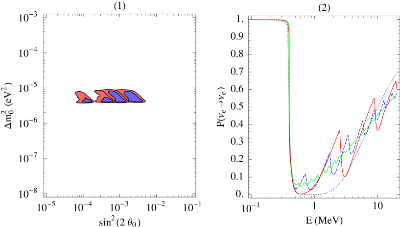
Figure 1: Fit of total rates in the $\sin^{2}2\theta_{0}$-${\Delta m^{2}_{\text{0}}}$ plane for different values of $1/R$. From right to left, the four patches correspond to $1/R=(20,5,2,0.5)\cdot 10^{-3}\,\mathrm{eV}$. The lighter (darker) regions represent the 99% (90%) CL.

Figure 2: Survival probabilities for $\mu_{e}\simeq 2.1\cdot 10^{-3}\,\mathrm{eV}$ and $(1/R,m_{e})=(20,0.058)\cdot 10^{-3}\,\mathrm{eV}$ (dotted line), $(1/R,m_{e})=(5,0.035)\cdot 10^{-3}\,\mathrm{eV}$ (darker solid line), $(1/R,m_{e})=(2,0.023)\cdot 10^{-3}\,\mathrm{eV}$ (dashed line) and $(1/R,m_{e})=(0.5,0.012)\cdot 10^{-3}\,\mathrm{eV}$ (lighter solid line).

In order to understand the main features of Fig. 2, in Fig. 2 we show the survival probabilities associated to the four values of $1/R$. The other two parameters $\mu_{e}$ and $m_{e}$ have been chosen in the corresponding best fit regions in Fig. 2. In particular, for all curves we have used $\mu_{e}\simeq 2.1\cdot 10^{-3}\,\mathrm{eV}$. In fact, as Fig. 2 shows, the allowed range for $\mu_{e}$ is independent of $1/R$ in first approximation. This is because $\mu_{e}$ defines the energy $E\sim\mu_{e}^{2}/(2V_{\text{c}})$ at which solar neutrinos start undergoing resonant conversion. Here, $V_{\text{c}}$ is the matter induced potential in the core of the sun. The parameter $\mu_{e}$ must therefore be in the range $\mu_{e}\sim(2\,\text{--}\,3)\cdot 10^{-3}\,\mathrm{eV}$ to ensure that Beryllium neutrinos are converted but $pp$-neutrinos are not.

Let us first consider the “large $1/R$” case $1/R=0.02\,\mathrm{eV}$, illustrated by the dotted line in Fig. 2. In this case, the resonant mixing between the electron doublet neutrino and the sterile tower will be significant only for the lowest state $N_{0}$, whose squared mass difference with the lightest state is ${\Delta m^{2}_{\text{0}}}=\mu^{2}_{e}$. This is because $2EV_{\text{c}}<{\Delta m^{2}_{\text{1}}}=\mu_{e}^{2}+1/R^{2}$ for any solar neutrino energy. The phenomenology of this case is the same as the one in models with a single sterile neutrino — the Kaluza Klein origin makes no difference. The precise value of $1/R$ does not really matter as long as $1/R\gtrsim 7\mu_{e}$. On the other hand, $m_{e}$ determines the mixing angle $\theta_{0}$ and hence the slope of the curve at the larger energies in Fig. 2. The chosen value is $m_{e}\simeq 0.58\cdot 10^{-4}\,\mathrm{eV}$ and it corresponds to $\sin^{2}2\theta_{0}\simeq 0.003$.

The darker solid line represents the particularly interesting case $1/R\simeq 5\cdot 10^{-3}\,\mathrm{eV}$ in which, besides the light state ${\hat{\nu}}$, three bulk states, $N_{0}$, $N_{1}$ and $N_{2}$, are involved in solar neutrino oscillation. The survival probability falls after each resonant energy since one more level has to be crossed by the neutrino on his way to the earth to be detected as an electron neutrino. This is compensated by the stronger raise between subsequent resonances, so that the prediction for the measured total rates is approximately the same as in the previous case. Such an higher slope is obtained by using a smaller mixing, namely $\sin^{2}2\theta_{0}\simeq 0.001$, corresponding to $m_{e}\simeq 0.35\cdot 10^{-4}\,\mathrm{eV}$. It is then clear why the allowed regions in Fig. 2 move towards the left for smaller $1/R$.

The dashed line corresponds to $\mu_{e}R\simeq 1$, $m_{e}\simeq 0.23\cdot 10^{-4}\,\mathrm{eV}$. This situation is similar to that analyzed by Smirnov and Dvali [13]. However, the splitting between the low-lying levels is not constant as in their model but is rather governed by eq. (5). As a consequence, the energy dependence of the survival probability near its minimum is slightly different. Finally, the light solid line corresponds to a case in which $\mu_{e}R>1$: $1/R\simeq 0.5\cdot 10^{-3}\,\mathrm{eV}$, $m_{e}\simeq 0.12\cdot 10^{-4}\,\mathrm{eV}$. A relatively large number of levels can now undergo resonant conversion. The single resonances are almost invisible because of the averaging over the neutrino production point in the sun.

So far we have compared the prediction of the model with the data on total rates only. Recently, the SK collaboration has claimed that their data on the recoil energy spectrum and day-night asymmetry allow to disfavour oscillations of solar neutrinos into a single sterile neutrino and into an active neutrino through the small mixing angle MSW mechanism. This conclusion depends on the way rates and energy spectrum are combined in a global fit. In what follows, we will quote confidence levels for total rates and energy spectrum separately. Whatever is the procedure followed, we now show that oscillations into more than one sterile neutrino are not only still allowed, but also fit particularly well the measured spectrum. The energy spectra associated with the four survival probabilities in Fig. 2 are shown in Fig. 4. The predictions are compared with the latest data [23, 8]. The dotted histogram again corresponds to the large $1/R$ regime equivalent to the case of a single sterile neutrino. Since it has the highest slope, it gives the worst fit of the energy spectrum and is unacceptable at 95% CL (free normalization). However, it is possible to find a better agreement with the energy spectrum for mixing angles at the lower border of the 90% allowed region in Fig. 2. The day-night asymmetry disfavours such lower angles for active neutrino oscillations, but does not play a crucial role in the sterile case.

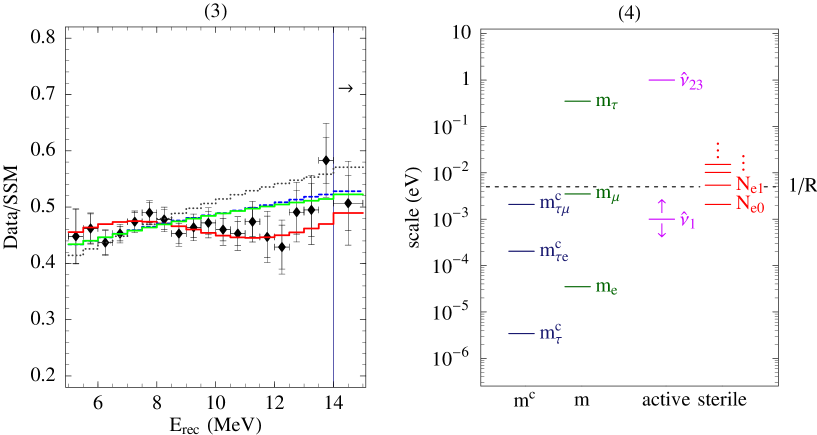
Figure 3: Energy spectra associated to the four survival probabilities in Fig. 2

Figure 4: Possible choice of parameters that allows to account for the solar, atmospheric and LSND oscillation signals. The scales corresponding to the mainly active neutrinos ${\hat{\nu}}_{1,2,3}$ and to the mainly sterile neutrinos $N_{en}$, $N_{\mu n}$, $N_{\tau n}$ are shown on the right hand side. Also shown are the scales of the lepton number conserving parameters $m_{e,\mu,\tau}$ and of the lepton number violating parameters $m^{c}_{\tau\mu,\tau\tau,\tau e}$.

The presence of additional sterile states reduces the slope of the predicted energy spectrum. This is illustrated by the (almost coincident) dashed and light solid histograms, corresponding to the two small $1/R$ cases in Fig. 2. The lower overall slope of the probabilities is also clearly visible there (the asymptotic behaviour for large $E$ has been discussed in [13]). The integration over the neutrino energy and the convolution with the detector resolution smear out the difference between the survival probabilities in Fig. 2. Quantitatively, the dashed and dotted lines agree pretty well with the measured spectrum. For the $1/R=0.002\,\mathrm{eV}$ histogram, for example, the fits of both total rates and energy spectrum are acceptable at 50% CL.

Finally, the darker solid line in Fig. 4 shows that the corresponding survival probability in Fig. 2 beautifully fits the energy spectrum. In this case, the fit of total rates and energy spectrum are already acceptable at the 25% and 10% CL respectively. The total $\chi^{2}$ is 11 for 21 data points.

Unlike the energy spectrum, the day-night asymmetry [24, 8] does not discriminate between the different possibilities discussed. In fact, the day-night asymmetry turns out to be small compared to the experimental errors in all cases considered above. Small earth effects affect the “midnight” bin only, where they can suppress the neutrino flux by a factor ranging from 0 to 0.5%. The day-night asymmetry for sterile neutrinos is smaller than for active ones for at least two reasons. First, the matter induced potential in the earth is smaller than for active neutrinos by more than a factor two. As a consequence, the MSW resonance takes place at higher energies, where the neutrino flux is smaller. Moreover, a larger resonant energy corresponds to a larger resonant wavelength and therefore, for a given length travelled in the earth, to a smaller oscillating term. We consider a small day-night asymmetry in reasonably good agreement with the present data, given that SK finds only a $1.2\,\sigma$ deviation from zero asymmetry.

The scenario discussed leads to various experimental signatures. First of all, a crucial test will be provided by the neutral/charged current ratio measurement in SNO [25]. Moreover, different sterile neutrino scenarios can be distinguished by the shape of the energy spectrum. As discussed, the present data already favours a flatter spectrum, which can be obtained if more than one sterile neutrino takes part in the oscillations. The charged current spectrum that will be measured by SNO could provide additional information. Finally, the measurement of a day-night asymmetry significantly lower than zero would disfavour the scenario with many sterile neutrinos.

Before discussing how this fits into a complete three generation model we briefly discuss the bounds on bulk neutrinos that come from the requirement that cooling in supernova due to bulk sterile neutrino emission should not be greater than the energy carried off by ordinary neutrinos. A more detailed discussion will be given in reference [26]. The most efficient mechanism for producing sterile neutrinos in supernova is resonant conversion [14]. The neutrino effective potential, $V$, in the supernova core is of order $10\,\mathrm{eV}$, giving a resonant mass $M_{n}\simeq n/R\simeq(2VE)^{1/2}\simeq 5\cdot 10^{4}\,\mathrm{eV}\,(E/100\,\mathrm{MeV})^{1/2}$ for a neutrino energy $E$. The effect of oscillation by resonant conversion can be reliably estimated for small mixing angles, because the width of each resonance is smaller than the separation between resonances. Thus the survival probability for a standard neutrino produced in the core is given by the product of the survival probabilities in crossing each resonance $P_{\nu\nu}\simeq\Pi_{n}P_{n}$, where $P_{n}\simeq e^{-\pi\gamma_{n}/2}$,

$$\gamma_{n}\simeq\frac{4m^{2}}{E}\frac{V}{dV/dr}\;,$$ (9)

and $m$ is the brane bulk mass. Following [14], we approximate the density profile by $\rho(r)\propto e^{-r/r_{\text{core}}}$. This gives $V/(dV/dr)=r_{\text{core}}\simeq 10^{6}\,\text{cm}$ and hence $\gamma_{n}\simeq m^{2}/(10^{-3}\,\mathrm{eV}^{2})\cdot(100\,\mathrm{MeV}/E)$. To determine the energy loss due to coherent processes we must determine the survival probability of the active neutrino after production by the process $e^{+}e^{-}\rightarrow\nu\overline{\nu}$. The initial energy of the neutrinos is roughly eight times the temperature. Subsequent scattering of the neutrino by thermalisation processes rapidly reduce its energy. The production rate is very rapid and neutrinos quickly reach their thermal equilibrium abundance (at $T=10\,\mathrm{MeV}$ this is achieved in $0.1\,\text{ms}$). Thereafter thermal processes limit the neutrinos to their thermal abundance. To good approximation the resonant conversion occurs only over the first few thermal path lengths, before annihilation processes eliminate the neutrino. Thus, after production, the survival probability will be $1-(\pi/2)\delta n\,\gamma_{n}$, where $\delta n$ is the number of levels crossed in one path length, $\delta n\simeq$ $(\delta\rho/2\rho)M_{n}R$, $\delta\rho/\rho=\lambda(T,E)/r_{\text{core}}$, where $\lambda(T,E_{\nu})$ is the mean path length for a neutrino of energy $E$ before annihilation. Putting all this together one finds the energy carried off by sterile neutrinos (again the dominant losses occur at the high initial temperature during the first second)

$$\epsilon = \frac{\pi}{2}\,\frac{1}{2}\,\frac{1}{2}\int\frac{dQ_{e}(E,T)}{dE}\,\mathcal{V}\,\delta n\,\gamma_{n}\,dE$$

$$\simeq 8\cdot 10^{61}\left(\frac{m^{2}R}{\,\mathrm{eV}}\right)\left(\frac{T}{30\,\mathrm{MeV}}\right)^{3.5}\;\text{erg}\;\text{s}^{-1}\;,$$

where $\mathcal{V}$ is the volume of the core and $dQ_{e}(E,T)/dE$ is the $e^{+}e^{-}\rightarrow\nu\overline{\nu}$ rate given by

$$Q_{e}=\int\frac{dQ_{e}(E,T)}{dE}dE\simeq 1.06\cdot 10^{25}\left(\frac{T}{\,\mathrm{MeV}}\right)^{9}\text{erg}\;\text{cm}^{-3}\;\text{s}^{-1}\;.$$

Requiring that $\epsilon$ be less than the energy carried off by neutrinos gives the bound

$$\left(\frac{m^{2}R}{\,\mathrm{eV}}\right)<3\cdot 10^{-8}\left(\frac{30\,\mathrm{MeV}}{T}\right)^{3.5}\;.$$ (11)

For the cases discussed above with $(1/R,m_{e})=(20,0.058)\cdot 10^{-3}\,\mathrm{eV}$, $(5,0.035)\cdot 10^{-3}\,\mathrm{eV}$, $(2,0.023)\cdot 10^{-3}\,\mathrm{eV}$ and $(0.5,0.012)\cdot 10^{-3}\,\mathrm{eV}$, this bound is satisfied for $T$ quite close to $30\,\mathrm{MeV}$. Thus we conclude that a solution to the solar neutrino problem involving oscillation to bulk Kaluza Klein states is just consistent with a supernova bounds. However it is clear that the large angle MSW and vacuum solutions are ruled out by the supernova bound as is the large angle atmospheric oscillation into sterile bulk states.

The discussion above shows that the mixing of the electron neutrino with a bulk fermion provides a “small mixing angle” sterile neutrino solution of the solar neutrino problem in good agreement with the present data. We now describe a model capable of explaining both solar and atmosheric oscillations in which the solar oscillation is predominantly due to oscillation from $\nu_{e}$ to a sterile KK tower as explained above and atmospheric neutrino oscillation is predominantly due to oscillation from $\nu_{\mu}$ to $\nu_{\tau}$. Indeed, in the perturbative regime specified in eq. (6), the bulk component of the SM neutrinos is too small to significantly affect the depletion of atmospheric neutrinos.

The light masses and the MNS mixing matrix $U$ are determined by the light mass matrix $m^{l}$ in (8). The simplest texture leading to maximal $\nu_{\mu}\leftrightarrow\nu_{\tau}$ oscillations is

$$m^{l}=\begin{pmatrix}\epsilon_{e}&\epsilon_{e\mu}&\epsilon_{e\tau}\\ \epsilon_{e\mu}&\epsilon_{\mu}&1\\ \epsilon_{e\tau}&1&\epsilon_{\tau}\end{pmatrix}\;m_{\mu\tau}\;,$$ (12)

where the $\epsilon$ parameters are much smaller than 1. In the limit in which the $\epsilon$ parameters are vanishing, the muon and tau neutrinos are superpositions of two degenerate states ${\hat{\nu}}_{2}$ and ${\hat{\nu}}_{3}$ with mass $|m_{\mu\tau}|$. The small $\epsilon_{\mu,\tau}$ parameters (assumed real for simplicity) are necessary to generate a mass splitting

$$\Delta m_{23}\simeq\epsilon\,|m_{\mu\tau}|,\qquad\epsilon=\epsilon_{\mu}+\epsilon_{\tau}$$

between the degenerate states and therefore an “atmospheric” squared mass difference ${\Delta m^{2}_{\text{ATM}}}={\Delta m^{2}_{\text{23}}}\simeq 2\epsilon|m_{\mu\tau}|^{2}$. The corresponding mixing angle $\theta_{\mu\tau}$ is almost maximal, $\sin^{2}2\theta_{\mu\tau}\simeq 1-(\epsilon_{\mu}-\epsilon_{\tau})^{2}/4$. The $\epsilon_{e\mu}$, $\epsilon_{e\tau}$ parameters are constrained to be small by the $\nu_{e}$ disappearance experiments.

Notice that the simple mechanism used here to generate a maximal $\nu_{\mu}\leftrightarrow\nu_{\tau}$ mixing does not work in a three neutrino scenario aiming at explaining at the same time the solar neutrino data. This is because the other two squared mass differences available turn out to be larger than the atmospheric one, unless all neutrino masses are very nearly degenerate [27]. As a consequence, for non-degenerate neutrinos, there is no room for the small ${\Delta m^{2}_{\text{}}}$ required by the solar data.

If the texture (12) accounts for atmospheric neutrino oscillations, the two degenerate neutrinos can provide a cosmologically significant source of dark matter. Moreover, the electron neutrino can oscillate into muon or tau neutrinos with a squared mass difference ${\Delta m^{2}_{\text{}}}>{\Delta m^{2}_{\text{ATM}}}$ and small amplitudes $2(\epsilon_{e\mu}\pm\epsilon_{e\tau})^{2}$ respectively. It is obviously tempting to associate such oscillations with the LSND signal. The MiniBooNE experiment will test this possibility and will cover a relevant portion of the parameter space for such short-baseline oscillations. A short-baseline neutrino factory could further extend the sensitivity in the $\epsilon_{e\mu}$ mixing parameter [28].

Let us now see how the texture (12) can be obtained. We consider a model with three towers of sterile neutrinos to match the three families of doublet neutrinos. One tower is coupled to the electron neutrino and generates solar neutrino oscillation as discussed in the previous Section. The remaining two towers do not play a direct role in neutrino oscillation and must be heavy. We assume that the bulk fermions $\Psi_{e,\mu,\tau}$ have the same individual lepton numbers $L_{e,\mu,\tau}$ as the corresponding neutrinos. The zero order form of eq. (12) in which the $\epsilon$ parameters vanish then simply follows from a first stage of lepton number breaking which leaves $L_{\mu}-L_{\tau}$ and $L_{e}$ unbroken. A further breaking of $L_{\mu}-L_{\tau}$ and $L_{e}$ finally generates the small entries in (12). For simplicity we break lepton number through the brane-bulk couplings $h^{c}$ in eq. (2) only.

The most general $L_{\mu}-L_{\tau}$ and $L_{e}$ conserving structure of the mass matrices $m$ and $m^{c}$ is

$$\begin{matrix}\phantom{{m}=\,\begin{matrix}\Psi_{\tau}\end{matrix}\,\;}\begin{matrix}\makebox[11.38765pt]{$\nu_{e}$}&\makebox[12.1544pt]{$\nu_{\mu}$}&\makebox[11.2282pt]{$\nu_{\tau}$}\end{matrix}\\[2.84526pt] {m}=\,\begin{matrix}\Psi_{e}\\ \Psi_{\mu}\\ \Psi_{\tau}\\ \end{matrix}\,\begin{pmatrix}m_{e}&0&0\\ 0&m_{\mu}&0\\ 0&0&m_{\tau}\end{pmatrix}\end{matrix}\qquad\begin{matrix}\phantom{{m^{c}}=\,\begin{matrix}\Psi^{c}_{\tau}\end{matrix}\,\;}\begin{matrix}\makebox[11.20357pt]{$\nu_{e}$}&\makebox[11.20357pt]{$\nu_{\mu}$}&\makebox[11.20357pt]{$\nu_{\tau}$}\end{matrix}\\[2.84526pt] {m^{c}}=\,\begin{matrix}\Psi^{c}_{e}\\ \Psi^{c}_{\mu}\\ \Psi^{c}_{\tau}\\ \end{matrix}\,\begin{pmatrix}\makebox[11.20357pt]{$0$}&0&0\\ 0&0&m^{c}_{\mu\tau}\\ 0&m^{c}_{\tau\mu}&0\end{pmatrix}\end{matrix}\;,$$ (13)

where $m_{e,\mu,\tau}$ can be made positive but $m^{c}_{\mu\tau}$ and $m^{c}_{\tau\mu}$ are in general complex. Moreover, the Dirac mass matrix of the bulk fields is diagonal, that is $\mu=\operatorname{Diag}(\mu_{e},\mu_{\mu},\mu_{\tau})$. The light mass matrix resulting from eq. (8) is then as given in eq. (12) with vanishing $\epsilon$ terms and $m_{\mu\tau}$ specified by

$$m_{\mu\tau}\simeq-\pi R\left(m_{\mu}m^{c}_{\mu\tau}\coth(\pi R\mu_{\mu})+m_{\tau}m^{c}_{\tau\mu}\coth(\pi R\mu_{\tau})\right)\;.$$ (14)

The LSND signal, if confirmed, would determine the size of $m_{\mu\tau}$ as $|m_{\mu\tau}|^{2}\simeq{\Delta m^{2}_{\text{LSND}}}$. The conditions eq. (6) for being in the perturbative regime become (taking also into account the U(1)-breaking)

$$\frac{\pi R|m_{e}|^{2}}{\mu_{e}}\coth(\pi R\mu_{e}) \ll 1$$ (15a)

$$\frac{\pi R|m_{\mu}|^{2}}{\mu_{\mu}}\coth(\pi R\mu_{\mu}) +\frac{\pi R|m^{c}_{\tau\mu}|^{2}}{\mu_{\tau}}\coth(\pi R\mu_{\tau})\ll 1$$ (15b)

$$\frac{\pi R|m_{\tau}|^{2}}{\mu_{\tau}}\coth(\pi R\mu_{\tau}) +\frac{\pi R|m^{c}_{\mu\tau}|^{2}}{\mu_{\mu}}\coth(\pi R\mu_{\tau})\ll 1\;.$$ (15c)

At this stage, the electron family is decoupled from the other two. The solar neutrino phenomenology is therefore given by the one family model described previously, where $\mu_{e}$ and $m_{e}$ are as discussed. As reference values for these parameters, we will, in the following, consider the best fit values $\mu_{e}\simeq 2.1\cdot 10^{-3}\,\mathrm{eV}$, $1/R=5\cdot 10^{-3}\,\mathrm{eV}$, $m_{e}\simeq 0.35\cdot 10^{-4}\,\mathrm{eV}$. To complete the picture, we only need to break $L_{\mu}-L_{\tau}$ in order to generate ${\Delta m^{2}_{\text{ATM}}}$ and to break $L_{e}$ in order to account for the LSND signal. This is easily accomplished by switching on the $L_{\mu}-L_{\tau}$ and $L_{e}$ violating entries in either $m$ or $m^{c}$ in eq. (13). This also adds to the electron neutrino a small $\Psi_{\mu}$ and $\Psi_{\tau}$ component. Such a component, however, does not affect the solar neutrino discussion since the squared mass difference with the lowest mode is too large to give rise to resonant conversion.

The possible combinations of parameters leading to viable models are numerous. With the only purpose of exhibiting an example, let us consider a case in which the lepton number conserving parameters $m_{e}$, $m_{\mu}$ and $m_{\tau}$ are hierarchical, with a gap of two orders of magnitude between “near” families and $m_{e}$ taking the reference values above. Similarly, we take for $\mu_{e}$ the value required by solar neutrino oscillations. The values for $\mu_{\mu}$ and $\mu_{\tau}$ do not affect the particle phenomenology of the model significantly as long as they are both larger than $1/R$ and smaller than the string scale. This is because, from eq. (8), the heavy mass scale that governs the see-saw suppression of the light masses is always given by $1/R$ for $\mu_{\mu}$ and $\mu_{\tau}$ in this range. As a consequence, we are free to choose for example $\mu_{\mu}$ and $\mu_{\tau}$ safely above $\sqrt{2EV}$, where $V$ is the matter potential in the core of a supernova and $E$ is the relevant neutrino energy as discussed above. This avoids any possible problem with the supernova bound eq. (11) due to conversion of $\mu$ or $\tau$ neutrinos into their associated Kaluza-Klein states.

In order to generate the LSND squared mass difference, $|m^{c}_{\tau\mu}|$ should be given by

$$\left|m^{c}_{\tau\mu}\right|\simeq 0.005\sqrt{{\Delta m^{2}_{\text{LSND}}}}\;,$$

where we have also assumed $|m^{c}_{\mu\tau}|\sim|m^{c}_{\tau\mu}|$. The atmospheric squared mass difference and the LSND mixing angle $\theta_{\text{LSND}}$ can, for example, be generated by a $m^{c}_{\tau}\overline{\Psi^{c}}_{\tau}\nu_{\tau}$ and a $m^{c}_{\tau e}\overline{\Psi^{c}}_{\tau}\nu_{e}$ mass term respectively, if

$$m^{c}_{\tau}=\frac{{\Delta m^{2}_{\text{ATM}}}}{4{\Delta m^{2}_{\text{LSND}}}}m^{c}_{\tau\mu}\quad\text{and}\quad m^{c}_{\tau e}=\frac{\sin 2\theta_{\text{LSND}}}{\sqrt{2}}\,m^{c}_{\tau\mu}\;.$$

Also, the perturbative conditions, eqs. (14), are satisfied.

The hierarchy of the various scales in this example is illustrated in Fig. 4 for ${\Delta m^{2}_{\text{LSND}}}\sim 1\,\mathrm{eV}^{2}$ and ${\Delta m^{2}_{\text{ATM}}}\sim 3\cdot 10^{-3}\,\mathrm{eV}^{2}$. Notice that the brane-bulk masses are given by $m_{i}\sim h_{i}(M_{\text{s}}/\,\mathrm{TeV})\,0.5\cdot 10^{-5}\,\mathrm{eV}$, where $h_{i}$, $i=e,\mu,\tau$, is the brane coupling of the $i$ family. Brane-bulk masses larger than $10^{-5}\,\mathrm{eV}$, as required in the above example, can arise from a string scale larger than $1\,\mathrm{TeV}$ or, alternatively, from large couplings $h_{i}$.

To summarise, we have studied the possibility that doublet neutrinos may oscillate into the sterile tower of Kaluza Klein states associated with bulk neutrinos, modulini, propagating in new large dimensions. The most stringent constraint comes from supernova and we found that large mixing angles between doublet neutrinos and light singlet bulk states are ruled out but that small mixing angles, of the order needed to explain solar neutrino oscillation, are allowed. A detailed study of the phenomenology associated with small angle MSW oscillation to a sterile Kaluza Klein tower shows that there is a much larger range of possibilities than has hitherto been explored. These arise if one allows for bulk masses in addition to the usual Kaluza Klein masses and allow for a range of different spacing between the bulk states. As a result one may go from the limit in which only a single bulk state is involved in the resonant conversion to the case where a continuum contributes. The former gives the same phenomenology as a single sterile neutrino and is disfavoured by the SK data for the energy spectrum and the total rates. However, if more bulk states contribute the deviation from the observed energy spectra reduces and an excellent fit to the data is possible for a level spacing in which three KK modes contribute significantly to the resonant oscillation. This model can readily be extended to describe all present indications of neutrino mass, including maximal mixing for atmospheric neutrinos in a natural way and the LSND signal. It can also give rise to a cosmologically significant dark matter component.

References

- [1] H. Sobel, Talk at the XIX International Conference on Neutrino Physics and Astrophysics (Neutrino 2000), Sudbury, Canada, June 16–21, 2000, http://nu2000.sno.laurentian.ca/H.Sobel/.
- [2] S. Hatakeyama et al., Kamiokande collaboration, Phys. Rev. Lett.81 (1998) 2016; M. Ambrosio et al., MACRO collaboration, Phys. Lett. B434 (1998) 451; M. Spurio, for the MACRO collaboration, hep-ex/9808001, talk given at the 16th European Cosmic Ray Symposium (ECRS), Alcala de Henares, Madrid, 20-25 Jul 1998.
- [3] K.S. Hirata et al., Kamiokande collaboration, Phys. Lett. B205 (1988) 416, Phys. Lett. B280 (1992) 146; E.W. Beier et al., Phys. Lett. B283 (1992) 446; Y. Fukuda et al., Kamiokande collaboration, Phys. Lett. B335 (1994) 237; K. Munakata et al., Kamiokande collaboration, Phys. Rev. D56 (1997) 23; Y. Oyama et al., Kamiokande collaboration, hep-ex/9706008; D. Casper et al., IMB collaboration, Phys. Rev. Lett. 66 (1991) 2561; R. Becker-Szendy et al., IMB collaboration, Phys. Rev. D46 (1992) 3720; W.W.M. Allison et al., Soudan-2 collaboration, Phys. Lett. B391 (1997) 491.
- [4] M. Apollonio et al., CHOOZ collaboration, Phys. Lett. B420 (1998) 397.
- [5] M.C. Gonzalez-Garcia et al., Nucl. Phys. B573 (2000) 3, hep-ph/9906469.
- [6] J.N. Bahcall, P.I. Krastev and A.Y. Smirnov, Phys. Lett. B477 (2000) 401, hep-ph/9911248.
- [7] http://www.sns.ias.edu/jnb/SNdata/.
- [8] Y. Suzuki, Talk at the XIX International Conference on Neutrino Physics and Astrophysics (Neutrino 2000), Sudbury, Canada, June 16–21, 2000, http://nu2000.sno.laurentian.ca/Y.Suzuki/.
- [9] C. Athanassopoulos et al., LSND Collaboration, Phys. Rev. C54 (1996) 2685; Phys. Rev. Lett. 77 (1996) 3082.
- [10] C. Athanassopoulos et al., LSND Collaboration, Phys. Rev. Lett. 81 (1998) 1774.
- [11] E.L. Wright et al., Astrophys. J. 396 (1992) L13; M. Davis et al., Nature 359 (1992) 393; A.N. Taylor and M. Rowan-Robinson, ibid. 359 (1992) 396; J. Primack, J. Holtzman, A. Klypin and D. O. Caldwell, Phys. Rev. Lett. 74 (1995) 2160; K.S. Babu, R.K. Schaefer and Q. Shafi, Phys. Rev. D53 (1996) 606.
- [12] K.R. Dienes, E. Dudas and T. Gherghetta, Nucl. Phys. B557 (1999) 25, hep-ph/9811428; N. Arkani-Hamed, S. Dimopoulos, G. Dvali, and J. March-Russell, Presented at SUSY 98 Conference, Oxford, England, 11–17 July 1998, hep-ph/9811448; G. Dvali and A.Y. Smirnov, Nucl. Phys. B563 (1999) 63, hep-ph/9904211.
- [13] A.E. Faraggi and M. Pospelov, Phys. Lett. B458 (1999) 237, hep-ph/9901299; A. Ioannisian and A. Pilaftsis, Phys. Rev. D62 (2000) 066001, hep-ph/9907522; R.N. Mohapatra, S. Nandi and A. Perez-Lorenzana, Phys. Lett. B466 (1999) 115, hep-ph/9907520; R.N. Mohapatra and A. Perez-Lorenzana, Nucl. Phys. B576 (2000) 466, hep-ph/9910474; A. Ioannisian and J.W.F. Valle, (1999), hep-ph/9911349; R.N. Mohapatra and A. Perez-Lorenzana, (2000), hep-ph/0006278.
- [14] R. Barbieri, P. Creminelli and A. Strumia, (2000), hep-ph/0002199.
- [15] A. Lukas and A. Romanino, (2000), hep-ph/0004130.
- [16] A. Lukas, P. Ramond, A. Romanino and G.G. Ross, in preparation.
- [17] Super-Kamiokande, Y. Suzuki, Nucl. Phys. Proc. Suppl. 77 (1999) 35.
- [18] B.T. Cleveland et al., Astrophys. J. 496 (1998) 505.
- [19] SAGE, J.N. Abdurashitov et al., Phys. Rev. C60 (1999) 055801, astro-ph/9907113.
- [20] GALLEX, W. Hampel et al., Phys. Lett. B447 (1999) 127.
- [21] GNO, M. Altmann et al., (2000), hep-ex/0006034.
- [22] J.N. Bahcall, S. Basu and M.H. Pinsonneault, Phys. Lett. B433 (1998) 1, astro-ph/9805135.
- [23] Super-Kamiokande, Y. Fukuda et al., Phys. Rev. Lett. 82 (1999) 2430, hep-ex/9812011.
- [24] Super-Kamiokande, Y. Fukuda et al., Phys. Rev. Lett. 82 (1999) 1810, hep-ex/9812009.
- [25] SNO, J. Boger et al., Nucl. Instrum. Meth. A449 (2000) 172, nucl-ex/9910016.
- [26] G.G. Ross and S. Sarkar, in preparation.
- [27] R. Barbieri et al., (1999), hep-ph/9901228.
- [28] V. Barger et al., (2000), hep-ph/0007181.