RELATIONSHIP BETWEEN THE QUARK CONDENSATE AND LOW-ENERGY $\pi\pi$ OBSERVABLES BEYOND $O(p^{4})$††thanks:   Work supported in part by the EEC-TMR Program, Contract N. CT98-0169 (EURODA$\Phi$NE)..

L. Girlanda
IFAE, Universitat AutΓ²noma de Barcelona, E-08193 Barcelona, Spain
Abstract

The two-flavor Gell-Mann–Oakes–Renner ratio is expressed in terms of low-energy $\pi\pi$ observables including the $O(p^{6})$ double chiral logarithms, computed in Generalized Chiral Perturbation Theory. It is found that their contribution is important and tends to compensate the one from the single chiral logarithms.

1 Introduction

Low-energy $\pi\pi$ scattering offers the rare possibility to test a fundamental property of the QCD vacuum, the strength of quark-antiquark condensation $\langle\bar{q}q\rangle$[1]. The knowledge of this quantity is crucial to understand the mechanism of spontaneous chiral symmetry breakdown (SB$\chi$S) in the Standard Model. The quark condensate, as every other order parameter, depends on the number of massless flavors $N_{f}$, and will in general experience a paramagnetic suppression as $N_{f}$ increases[2]. It turns out that what can actually be measured from low-energy $\pi\pi$ scattering is the quark condensate in the limit of two massless flavors, $N_{f}=2$. The question to be addressed is to which extent $N_{f}=2$ is close to a critical point where $\langle\bar{q}q\rangle$ disappears and chiral symmetry is eventually broken by higher-dimensional order parameters[3]. The proper framework to analyze phenomenologically the issue is provided by the generalized version of Chiral Perturbation Theory ($\chi$PT)[1] in the case of SU(2)$\times$SU(2) chiral symmetry. This is a reorganization of the standard expansion of $\chi$PT[4] in which the quark condensate parameter $B$ is considered formally as a small quantity, in order to account for the possibility that the linear and quadratic terms, in the expansion of the pion mass $M_{\pi}^{2}$ in powers of quark masses $m_{u}=m_{d}=\hat{m}$, be of the same order. The chiral counting is modified accordingly,

$$B\sim\hat{m}\sim O(p),\hskip 28.45274pt{\cal L}=\tilde{\cal L}^{(2)}+\tilde{\cal L}^{(3)}+\tilde{\cal L}^{(4)}+\ldots$$ (1)

with $\tilde{\cal L}^{(d)}$ containing additional terms, relegated in higher orders by the standard counting. The complete effective Lagrangian up to $O(p^{4})$ can be found in Refs.[5], together with its renormalization at 1 loop.

At present, the low-energy $\pi\pi$ phase-shifts are rather poorly known, but considerable improvements are expected to come soon from new high-luminosity $K_{e4}$ decays experiments, performed at Brookhaven and DA$\Phi$NE. These new data, together with the recent numerical solutions of Roy Equations[6], will allow to extract the two $S$-wave scattering lengths or, equivalently, the two parameters $\alpha$ and $\beta$, introduced in Ref.[7] and representing respectively the amplitude and the slope at the symmetrical point $s=t=u=4/3M_{\pi}^{2}$. In this perspective, we have established the relationship between the two-flavor quark condensate, expressed through the deviation from the Gell-Mann–Oakes–Renner relation,

$$x_{2}^{\mathrm{GOR}}=\frac{|2\hat{m}\langle\bar{q}q\rangle|}{F_{\pi}^{2}M_{\pi}^{2}},$$ (2)

and the parameters $\alpha$ and $\beta$, including the leading $O(p^{6})$ double logarithmic corrections to the 1-loop result of Generalized $\chi$PT.

2 Double chiral logs

Due to the smallness of the pion mass, double chiral logarithms are among the potentially most dangerous contributions at order $O(p^{6})$. As first pointed out in Ref.[8] they can be obtained from a 1-loop calculation, using the fact that, in the renormalization procedure, non-local divergences must cancel. Setting the space-time dimension $d=4+\omega$ to regulate the theory, all the low-energy constants (l.e.c.’s) of the generalized Lagrangian with $k$ derivatives and $n$ powers of the scalar source, $c_{(k,n)}$, have dimension $2-k-n$, except $F^{2}$ which has dimension $[F^{2}]=d-2$. We thus replace $F^{2}$ with $\mu^{2\omega}F^{2}$, making appear explicitly the scale parameter $\mu$ brought in by the regularization procedure. Since each loop involves a factor $F^{-2}$, the chiral expansion of a generic amplitude ${\cal A}$, apart from an overall dimensional factor, takes the form,

$${\cal A}\sim{\cal A}_{\mathrm{tree}}+\left(\frac{M_{\pi}}{\mu}\right)^{\omega}\sum_{i}P^{(1)}_{i}(c_{(k,n)})g_{i}^{\mathrm{1-loop}}+\left(\frac{M_{\pi}}{\mu}\right)^{2\omega}\sum_{i}P^{(2)}_{i}(c_{(k,n)})f_{i}^{\mathrm{2-loop}}+\ldots,$$ (3)

where $P_{i}^{1,2}$ are polynomials in the l.e.c.’s and $g_{i}$ and $f_{i}$ are loop-functions of the kinematical variables, expressed in terms of dimensionless quantities. After writing the Laurent expansions of the loop-functions and of the coupling constants,

$$f_{i}=\frac{f_{i,2}}{\omega^{2}}+\frac{f_{i,1}}{\omega}+f_{i,0}+\ldots,\hskip 28.45274ptg_{i}=\frac{g_{i,1}}{\omega}+g_{i,0}+\ldots,\hskip 28.45274ptc_{i}=\frac{\delta_{i}}{\omega}+c_{i}^{r}+\ldots,$$ (4)

and imposing the cancellation of the non-local divergences $\sim 1/\omega\log M_{\pi}$, one finds that the double chiral logarithms are given by the residues $g_{i,1}$ of the pole in $\omega$, and always occur in the same combination with the terms $\sim c_{i}^{r}\log(M_{\pi}/\mu)$,

$${\cal A}^{\mathrm{llogs}}\sim\frac{g_{i,1}}{8}\left[-\frac{\Gamma_{i}}{16\pi^{2}}\log\frac{M_{\pi}^{2}}{\mu^{2}}+4c_{i}^{r}\right]\log\frac{M_{\pi}^{2}}{\mu^{2}},$$ (5)

$\Gamma_{i}$ being the $\beta$-function coefficients of the l.e.c. $c_{i}$. Notice that at order $O(p^{6})$ we never have to deal with products like $\Gamma_{i}\Gamma_{j}$, since all 1-loop divergences are at least $O(p^{4})$. We display the result for $M_{\pi}$ and $F_{\pi}$, where all l.e.c.’s, here and in the following, are renormalized at a scale $\mu$:

$\displaystyle\frac{F_{\pi}^{2}}{F^{2}}M_{\pi}^{2}$ $\displaystyle=$ $\displaystyle 2B\hat{m}+4A\hat{m}^{2}+\left(9\rho_{1}+\rho_{2}+20\rho_{4}+2\rho_{5}\right)\hat{m}^{3}$ (6)
$\displaystyle+\left(16e_{1}+4e_{2}+32f_{1}+40f_{2}+8f_{3}+96f_{4}\right)\hat{m}^{4}$
$\displaystyle+4a_{3}M_{\pi}^{2}\hat{m}^{2}-\frac{M_{\pi}^{2}}{32\pi^{2}F_{\pi}^{2}}\left(3M_{\pi}^{2}+20A\hat{m}^{2}\right)\log\frac{M_{\pi}^{2}}{\mu^{2}}$
$\displaystyle+\left[\frac{33}{8}+\frac{65}{2}\frac{A\hat{m}^{2}}{M_{\pi}^{2}}+60\left(\frac{A\hat{m}^{2}}{M_{\pi}^{2}}\right)^{2}\right]M_{\pi}^{2}\left(\frac{M_{\pi}^{2}}{16\pi^{2}F_{\pi}^{2}}\log\frac{M_{\pi}^{2}}{\mu^{2}}\right)^{2},$
$\displaystyle F_{\pi}^{2}$ $\displaystyle=$ $\displaystyle F^{2}\left[1+2\xi^{(2)}\hat{m}+\left(2a_{1}+a_{2}+4a_{3}+2b_{1}-2b_{2}\right)\hat{m}^{2}-\frac{M_{\pi}^{2}}{8\pi^{2}F_{\pi}^{2}}\log\frac{M_{\pi}^{2}}{\mu^{2}}\right.$ (7)
$\displaystyle\left.+\frac{7}{2}\frac{M_{\pi}^{4}}{F_{\pi}^{4}}\left(\frac{1}{16\pi^{2}}\log\frac{M_{\pi}^{2}}{\mu^{2}}\right)^{2}\right].$

3 The GOR ratio

The amplitude for $\pi\pi$ scattering up to $O(p^{6})$ has been first given in Ref.[7], using dispersive techniques, independently of any assumption about the size of the chiral condensate. It can be expressed in terms of 6 parameters, $\alpha,\beta,\lambda_{1},...,\lambda_{4}$,

$$A(s|t,u)=A_{\mathrm{KMSF}}(s|t,u;\alpha,\beta;\lambda_{1},\lambda_{2},\lambda_{3},\lambda_{4})+O\left[\left({p\over\Lambda_{\mathrm{H}}}\right)^{8},\left({M_{\pi}\over\Lambda_{\mathrm{H}}}\right)^{8}\right].$$ (8)

The $\lambda_{i}$’s can be determined from a set of twice subtracted fixed-$t$ dispersion relations (Roy Equations), whereas $\alpha$ and $\beta$ can be related to the two subtraction constants. Most of the sensitivity to $\langle\bar{q}q\rangle$ is contained in the parameter $\alpha$, which, at tree level, varies from 1 to 4 if $\langle\bar{q}q\rangle$ is decreased from its standard value down to zero. The complete two-loop S$\chi$PT calculation of Ref.[9] allows in addition to express the six parameters in terms of the l.e.c.’s[10]. It is interesting to notice that, in this standard case, the double chiral logarithms constitute by far the largest $O(p^{6})$ contribution to $\alpha$. An explicit calculation in G$\chi$PT, along the lines described in the previous section, yields,

$\displaystyle\alpha$ $\displaystyle=$ $\displaystyle\frac{F^{2}}{F_{\pi}^{2}M_{\pi}^{2}}\biggl{[}2B\hat{m}+16A\hat{m}^{2}-4M_{\pi}^{2}\xi^{(2)}\hat{m}+\left(81\rho_{1}+\rho_{2}+164\rho_{4}+2\rho_{5}\right)\hat{m}^{3}$ (9)
$\displaystyle-8M_{\pi}^{2}\left(2b_{1}-2b_{2}-a_{3}-4c_{1}\right)\hat{m}^{2}$
$\displaystyle+16\left(6Aa_{3}+16e_{1}+e_{2}+32f_{1}+34f_{2}+2f_{3}+72f_{4}\right)\hat{m}^{4}$
$\displaystyle-\frac{M_{\pi}^{2}}{32\pi^{2}F_{\pi}^{2}}\left(4M_{\pi}^{2}+204A\hat{m}^{2}+528\frac{A^{2}\hat{m}^{4}}{M_{\pi}^{2}}\right)\log\frac{M_{\pi}^{2}}{\mu^{2}}$
$\displaystyle-\frac{1}{32\pi^{2}F_{\pi}^{2}}\left[M_{\pi}^{4}+88A\hat{m}^{2}M_{\pi}^{2}+528A^{2}\hat{m}^{4}\right]$
$\displaystyle+M_{\pi}^{2}\left[\frac{533}{72}+\frac{18817}{30}\frac{A\hat{m}^{2}}{M_{\pi}^{2}}+\frac{61076}{15}\left(\frac{A\hat{m}^{2}}{M_{\pi}^{2}}\right)^{2}\right.$
$\displaystyle\left.+5808\left(\frac{A\hat{m}^{2}}{M_{\pi}^{2}}\right)^{3}\right]\left(\frac{M_{\pi}^{2}}{16\pi^{2}F_{\pi}^{2}}\log\frac{M_{\pi}^{2}}{\mu^{2}}\right)^{2}\biggr{]},$
$\displaystyle\beta$ $\displaystyle=$ $\displaystyle 1+2\xi^{(2)}\hat{m}-4{\xi^{(2)}}^{2}\hat{m}^{2}+2\left(3a_{2}+2a_{3}+4b_{1}+2b_{2}+4c_{1}\right)\hat{m}^{2}$ (10)
$\displaystyle-\frac{4M_{\pi}^{2}}{32\pi^{2}F_{\pi}^{2}}\left(1+10\frac{A\hat{m}^{2}}{M_{\pi}^{2}}\right)\left(\log\frac{M_{\pi}^{2}}{\mu^{2}}+1\right)$
$\displaystyle+\left(\frac{151}{36}M_{\pi}^{4}+\frac{400}{3}M_{\pi}^{2}A\hat{m}^{2}+420A^{2}\hat{m}^{4}\right)\left[\frac{1}{16\pi^{2}F_{\pi}^{2}}\log\frac{M_{\pi}^{2}}{\mu^{2}}\right]^{2},$
$\displaystyle\lambda_{1}$ $\displaystyle=$ $\displaystyle 2l_{1}-\frac{1}{48\pi^{2}}\log\frac{M_{\pi}^{2}}{\mu^{2}}-\frac{1}{36\pi^{2}}+\left(\frac{25}{18}+\frac{130}{9}\frac{A\hat{m}^{2}}{M_{\pi}^{2}}\right)\left[\frac{M_{\pi}^{2}}{16\pi^{2}F_{\pi}^{2}}\log\frac{M_{\pi}^{2}}{\mu^{2}}\right]^{2},$ (11)
$\displaystyle\lambda_{2}$ $\displaystyle=$ $\displaystyle l_{2}-\frac{1}{48\pi^{2}}\log\frac{M_{\pi}^{2}}{\mu^{2}}-\frac{5}{288\pi^{2}}+\left(\frac{5}{3}+\frac{80}{9}\frac{A\hat{m}^{2}}{M_{\pi}^{2}}\right)\left[\frac{M_{\pi}^{2}}{16\pi^{2}F_{\pi}^{2}}\log\frac{M_{\pi}^{2}}{\mu^{2}}\right]^{2},$ (12)
$\displaystyle\lambda_{3}$ $\displaystyle=$ $\displaystyle\frac{10}{9}\left[\frac{1}{16\pi^{2}}\log\frac{M_{\pi}^{2}}{\mu^{2}}\right]^{2},\hskip 28.45274pt\lambda_{4}=-\frac{5}{18}\left[\frac{1}{16\pi^{2}}\log\frac{M_{\pi}^{2}}{\mu^{2}}\right]^{2}.$ (13)

It is easy to check that these formulae, when restricted to the standard case, agree with the ones displayed in Ref.[10] based on the complete two-loop calculation.
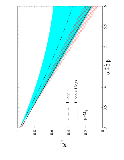
Refer to caption
Figure 1: The GOR ratio at 1 loop including (continuous) and not including (dashed) the double logarithms. The scale is set to $\mu=M_{\eta}\pm 250$ MeV.

Eliminating the constant $A$ in favor of $\alpha$ and $\xi^{(2)}$ in favor of $\beta$, one can express the GOR ratio of Eq. (2) as function of the combination $\alpha+2\beta$,

$\displaystyle x_{2}^{\mathrm{GOR}}$ $\displaystyle=$ $\displaystyle\frac{2\hat{m}BF^{2}}{F_{\pi}^{2}M_{\pi}^{2}}=2-\frac{\alpha+2\beta}{3}+\frac{F^{2}}{F_{\pi}^{2}M_{\pi}^{2}}\left(15\rho_{1}^{(2)}-\rho_{2}^{(2)}+28\rho_{4}^{(2)}-2\rho_{5}^{(2)}\right)\hat{m}^{3}$ (14)
$\displaystyle+\left[4a_{2}+8\left(\frac{\alpha+2\beta}{3}-1\right)a_{3}+8b_{2}+16c_{1}\right]\hat{m}^{2}$
$\displaystyle+\frac{64}{M_{\pi}^{2}}(e_{1}+2f_{1}+2f_{2}+4f_{4})\hat{m}^{4}+\frac{M_{\pi}^{2}}{288\pi^{2}F_{\pi}^{2}}\left(\alpha+2\beta\right)\left[24-11(\alpha+2\beta)\right]$
$\displaystyle+\left[6+\frac{5}{3}(\alpha+2\beta)-\frac{11}{9}(\alpha+2\beta)^{2}\right]\frac{M_{\pi}^{2}}{32\pi^{2}F_{\pi}^{2}}\log\frac{M_{\pi}^{2}}{\mu^{2}}+\left[\frac{11}{60}-\frac{4169}{1080}(\alpha+2\beta)\right.$
$\displaystyle\left.+\frac{5639}{1620}(\alpha+2\beta)^{2}-\frac{121}{108}(\alpha+2\beta)^{3}\right]\left(\frac{M_{\pi}^{2}}{16\pi^{2}F_{\pi}^{2}}\log\frac{M_{\pi}^{2}}{\mu^{2}}\right)^{2}.$

Fig. 1 shows this function for $\mu=M_{\eta}$. The upper left corner represents the standard case, corresponding to $\alpha\sim 1,\beta\sim 1$, while higher values for $\alpha+2\beta$ would imply a significant departure from that picture. The dashed line is the result without including the $O(p^{6})$ double logarithms. The bands are obtained varying the $\chi$PT scale by $\pm$250 MeV and treating the unknown l.e.c.’s as randomly distributed around zero with magnitude according to naΓ―ve dimensional analysis,

$$\rho_{i}\sim\frac{1}{\Lambda_{\mathrm{H}}},\hskip 56.9055pta_{i},b_{i},c_{i},e_{i},f_{i}\sim\frac{1}{\Lambda_{\mathrm{H}}^{2}}.$$ (15)

Most of the uncertainty comes from the $\mu$-dependence, which however, quite interestingly, almost cancels when including the double logarithms. The contribution from the latters is found to be rather large, although smaller that the $O(p^{4})$ one, and tends to compensate for the 1-loop shift. An additional uncertainty (of difficult estimation), from the remaining $O(p^{5},p^{6})$ pieces, should be understood in Fig. 1.

References

  • 1 . N.H. Fuchs, H. Sazdjian and J. Stern, Phys. Lett. B269 (1991), 183; Phys. Rev. D47 (1993), 3814;
    M. Knecht, B. Moussallam and J. Stern, in The Second Da$\Phi$ne Physics Handbook, eds. L. Maiani, G. Pancheri and N. Paver, 1995; hep-ph/9411259.
  • 2 . B. Moussallam, Eur. Phys. J. C14 (2000), 111 ; hep-ph/0005245.
    S. Descotes, L. Girlanda and J. Stern, JHEP 01 (2000), 41.
  • 3 . J. Stern, hep-ph/9801282.
  • 4 . J. Gasser and H. Leutwyler, Ann. Phys. (NY) 158 (1984), 142; Nucl. Phys. B250 (1985), 465.
  • 5 . L. Ametller, J. Kambor, M. Knecht and P. Talavera, Phys. Rev. D60 (1999), 094003.
    L. Girlanda and J. Stern, Nucl. Phys. B575 (2000), 285.
  • 6 . B. Ananthanarayan, G. Colangelo, J. Gasser and H. Leutwyler, hep-ph/0005297.
  • 7 . M. Knecht, B. Moussallam, J. Stern and N.H. Fuchs, Nucl. Phys. B457 (1995), 513; Nucl. Phys. B471 (1996), 445.
  • 8 . S. Bellucci, J. Gasser and M.E. Sainio, Nucl. Phys. B423 (1994), 80.
  • 9 . J. Bijnens, G. Colangelo, G. Ecker, J. Gasser and M. Sainio, Phys. Lett. B374 (1996), 210; Nucl. Phys. B508 (1997), 263.
  • 10 . L. Girlanda, M. Knecht, B. Moussallam and J. Stern, Phys. Lett. B409 (1997), 461.