A phase-space generation algorithm, capable to efficiently integrate the squared amplitude of any scattering process, is presented. The algorithm has been implemented in a Monte Carlo program, PHEGAS, which, using HELAC, a helicity amplitude computational package, can be used for automatic cross-section computation and event generation. Results for several scattering processes with four, five and six particles in the final state are briefly presented.

July 2000

The study of multi-particle processes, like for instance four-fermion production in $e^{+}e^{-}$, requires efficient phase-space Monte Carlo generators. The reason is that the squared amplitude, being a complicated function of the kinemtaical variables, exhibits strong variations in specific regions and/or directions of the phase space, lowering in a substantial way the speed and the efficiency of the Monte Carlo integration. A well known way out of this problem relies on algorithms characterized by two main ingredients:

1. The construction of appropriate mappings of the phase space parametrization in such a way that the main variation of the integrand can be described by a set of almost uncorrelated variables, and

2. A self-adaptation procedure that reshapes the generated phase-space density in order to be as much as possible close to the integrand.

Up to now such algorithms have been developed in several cases to deal with specific processes, like four-fermion [1], four-fermion plus a photon [2, 10, 11] and six fermion [3] production in $e^{+}e^{-}$ collisions, as well as in the framework of general-purpose computational packages like CompHEP [4] and GRACE [5]. It is the aim of this letter to present a generalized recursive algorithm, together with its implementation, that can be used for automatic cross-section computation for any multi-particle process.

In order to construct appropriate mappings we note that the integrand, i.e. the squared amplitude, has a well-defined representation in terms of Feynman diagrams. It is therefore natural to associate to each Feynman diagram a phase-space mapping that parametrizes the leading variation coming from it. To be more specific the contribution of tree-order Feynman diagrams to the full amplitude can be factorized in terms of propagators, vertex factors and external wave functions. In general, the main source of variation comes from the propagator factors and therefore our aim is to construct a mapping that expresses the phase-space density in terms of the kinematical invariants that appear in these propagator factors. Since in principle we need as many mappings as Feynman diagrams for the process under consideration, we have to appropriately combine them in order to produce the global phase-space density. A simple and well studied solution to this problem was suggested some time ago in reference [6]. Let us represent the normalized phase space-density of a mapping by a function $g_{i}(\Phi)$ where $\Phi$ refers to the $(3n-4)$-dimensional phase space, $n$ being the number of produced particles. The overall density can be represented by

$$g(\Phi)=\sum_{i=1}^{M}\alpha_{i}g_{i}(\Phi)$$

where

$$0<\alpha_{i}<1\;\;\;\;\;\sum_{i=1}^{M}\alpha_{i}=1$$

and $M$ is the total number of mappings. Since the result of the integration does not depend on the specific values of $\alpha_{i}$, the so-called a priori weights, the latter can be used to optimize the Monte Carlo integration. A self-adaptation procedure therefore suggests itself: during the evaluation of the integral, $\alpha_{i}$ are repeatedly redefined [6], so that the variance of the integrand is minimized. It should be mentioned however that other self-adapting approaches can be used as well [7].

In order to describe the construction of the phase-space mappings, let us consider a typical process in which two incoming particles produce $n$ outgoing ones. The phase space can be represented by

$$d\Phi_{n}(P;p_{1}\ldots,p_{n})=(2\pi)^{4-3n}\delta^{4}\left(\sum_{i=1}^{n}p_{i}-P\right)\prod_{i=1}^{n}d^{4}p_{i}\;\delta(p_{i}^{2}-m_{i}^{2})$$ (1)

where $P=q_{1}+q_{2}$ with $q_{1}$, $q_{2}$ being the momenta of the incoming particles.

A well known property of Eq.(1) is that the phase space can be decomposed as follows

$$d\Phi_{n}(P;p_{1},p_{2},\ldots,p_{n}) = \left(\prod_{i=1}^{m}\frac{dQ_{i}^{2}}{2\pi}\right)d\Phi_{m}(P;Q_{1},\ldots,Q_{m})$$ (2)

$$d\Phi_{n_{1}}(Q_{1};r_{1},r_{2},\ldots,r_{n_{1}})\ldots d\Phi_{n_{m}}(Q_{m};s_{1},s_{2},\ldots,s_{n_{m}})$$

where the subsets $\{r_{1},r_{2},\ldots,r_{n_{1}}\}$ up to $\{s_{1},s_{2},\ldots,s_{n_{m}}\}$ represent an arbitrary partition of $\{p_{1},p_{2},\ldots,p_{n}\}$. The above equation can be generalized recursively resulting in an arbitrary decomposition of $d\Phi_{n}$. Feynman graphs can be seen as a realization of such a decomposition, this latter being identified with a sequence of vertices of the graph. For instance a three-particle vertex $V=(Q\to Q_{1},Q_{2})$ in a Feynman diagram can be seen as part of the phase-space decomposition

$$d\Phi_{n}=\ldots\frac{dQ_{1}^{2}}{2\pi}\;\frac{dQ_{2}^{2}}{2\pi}\;d\Phi_{2}(Q;Q_{1},Q_{2})\ldots\;\;\;.$$ (3)

The appropriate sequence of vertices, $\{V_{1},V_{2},\ldots,V_{k}\}$ can be chosen in such a way that a recursive construction of the phase space is realized. For instance $V_{1}$ should contain at least one incoming particle whose momentum is known. The rest of the sequence is chosen recursively: vertex $V_{j}$ is characterized by an incoming momentum $Q$ which has already been generated in one of the $\{V_{1},\ldots,V_{j-1}\}$ and outgoing momenta $Q_{1}$ and $Q_{2}$ that are generated according to Eq.(3).

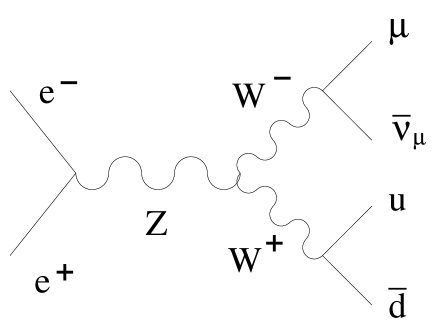
Figure 1: Feynman graph contributing to $e^{-}\;e^{+}\to\mu^{-}\;\bar{\nu}_{\mu}\;u\;\bar{d}$.

As a more illustrative example let us consider the graph of Fig.1 for the process

$$e^{-}(q_{1})\;e^{+}(q_{2})\to\mu^{-}(p_{1})\;\bar{\nu}_{\mu}(p_{2})\;u(p_{3})\;\bar{d}(p_{4})$$

The appropriate sequence of vertices can be chosen as

$$V_{1}=(q_{1}\to-q_{2},Q),V_{2}=(Q\to Q_{1},Q_{2}),V_{3}=(Q_{1}\to p_{1},p_{2}),V_{4}=(Q_{2}\to p_{3},p_{4})$$

where $Q,Q_{1},Q_{2}$ are the momenta of $Z,W^{-},W^{+}$ respectively. In the first vertex, $V_{1}$, both $q_{1}$ and $q_{2}$ are considered known so this is a mere definition of $Q=q_{1}+q_{2}$. The rest of the sequence realizes the following phase-space decomposition

$$d\Phi_{4}(q_{1}+q_{2};p_{1},p_{2},p_{3},p_{4}) = d\Phi_{2}(q_{1}+q_{2};Q_{1},Q_{2})$$ (4)

$$\frac{dQ_{1}^{2}}{2\pi}\frac{dQ_{2}^{2}}{2\pi}$$

$$d\Phi_{2}(Q_{1};p_{1},p_{2})$$

$$d\Phi_{2}(Q_{2};p_{3},p_{4})$$

allowing for the correct treatment of the Breit-Wigner propagators of $W^{\pm}$ in terms of the variables $Q_{1}^{2}$ and $Q_{2}^{2}$.

In the general case one can distinguish two types of vertices:

1. All outgoing momenta involved in the vertex are time-like.

2. One of them is space-like.

It is worthwhile to mention that for $2\to n$ scattering these two cases are the only possible ones.

For the first case the phase space decomposition can be written as

$$d\Phi_{n} = \ldots\frac{dQ_{1}^{2}}{2\pi}\;\frac{dQ_{2}^{2}}{2\pi}\;d\Phi_{2}(Q\to Q_{1},Q_{2})\ldots$$

$$= \ldots\frac{dQ_{1}^{2}}{2\pi}\;\frac{dQ_{2}^{2}}{2\pi}\;d\cos\theta\;d\phi\;\frac{\lambda^{1/2}(Q^{2},Q_{1}^{2},Q_{2}^{2})}{32\pi^{2}\;Q^{2}}\ldots$$

$$\lambda(x,y,z)=x^{2}+y^{2}+z^{2}-2xy-2xz-2yz$$

with the understanding that whenever $Q_{1}$ or $Q_{2}$ represents an external momentum the corresponding factor $dQ_{i}^{2}/2\pi$ is set to $1$. Generation can now proceed straightforwardly, by first generating $Q_{1}^{2}$ and $Q_{2}^{2}$ using any prescribed density, as well as $\cos\theta$ and $\phi$ in the rest frame of $Q$. Then by using the known momentum $Q$ a boost to the initial frame can be performed. As it is easily seen the first case results to a rather simple generation algorithm.

The second case is more involved. The phase space is decomposed as follows:

$$d\Phi_{n} = \ldots\frac{dQ_{1}^{2}}{2\pi}\;\frac{dQ_{2}^{2}}{2\pi}\;d\Phi_{2}(Q\to Q_{1},Q_{2})\ldots$$ (5)

$$= \ldots\frac{dQ_{1}^{2}}{2\pi}\;\frac{dQ_{2}^{2}}{2\pi}\;dt\;d\phi\;\frac{1}{32\pi^{2}\;Q\;|\vec{q}_{2}|}\ldots$$

with

$$t=(Q_{1}-q_{2})^{2}=m_{2}^{2}+Q_{1}^{2}-\frac{E_{2}}{Q}(Q^{2}+Q_{1}^{2}-Q_{2}^{2})+\frac{\lambda^{1/2}}{Q}|\vec{q}_{2}|\cos\theta$$

and $(E_{2},\vec{q}_{2})$ being the incoming momentum $q_{2}$ in the rest frame of $Q$. In order to have an efficient generation according to Eq.(5) we need to know the limits of the $t-$ and $Q_{1}^{2}-$integration: a detailed presentation of their derivation can be found in the Appendix.

Although in the two cases described so far we used a three-particle vertex the algorithm can be generalized in a straightforward way in the case of a four-particle vertex, either using the three-body phase space explicitly

$$d\Phi_{n}=\ldots\frac{dQ_{1}^{2}}{2\pi}\;\frac{dQ_{2}^{2}}{2\pi}\;\frac{dQ_{3}^{2}}{2\pi}\;d\Phi_{3}(Q\to Q_{1},Q_{2},Q_{3})\ldots$$

in the case all momenta are time-like, or using

$$d\Phi_{n}=\ldots\frac{dQ_{1}^{2}}{2\pi}\;\frac{dQ_{23}^{2}}{2\pi}\;d\Phi_{2}(Q\to Q_{1},Q_{23})$$

followed by

$$\ldots\frac{dQ_{2}^{2}}{2\pi}\;\frac{dQ_{3}^{2}}{2\pi}d\Phi_{2}(Q_{23}\to Q_{2},Q_{3})\ldots$$

in the case one space-like outgoing momentum is present.

Following the above described algorithm we end up with an expression for the phase-space density,

$$d\Phi_{n}\to\prod ds_{i}\;\prod dt_{j}\;\prod d\phi_{k}\prod d\cos\theta_{l}$$ (6)

where $s_{i}$ and $t_{j}$ refer to the kinematical invariants entering the propagator factors of the graph and $\phi_{k}$ and $\cos\theta_{l}$ represent center-of-mass angles needed to complete the phase space parametrization. It is now straightforward to generate $s_{i}$ and $t_{j}$ with a probability density given by:

• $p(x)\sim(x-m^{2})^{2}+m^{2}\Gamma^{2}$

  for massive unstable particles, like $W^{\pm}$, $Z$, $t$ .

• $p(x)\sim x^{\nu}$

  for time-like massless propagators, e.g. $\gamma$, gluons, massless fermions.

• $p(x)\sim|x|^{\nu}$

  for space-like massless propagators.

so that the corresponding propagator factor cancels out in the Monte Carlo weight. The value of the exponent $\nu$, for $\gamma$ and gluons, is chosen very close to 1 in order to account for the leading single-pole behaviour of the squared amplitude as a result of the gauge cancellations.

The implementation of this algorithm, called PHEGAS, is based on and combined with HELAC [8] a package that computes any tree-order matrix element. HELAC is based on the Dyson-Schwinger recursive equations that proved to be superior to the Feynman diagram representation for amplitude computation. On the other hand it is still an open problem how to use Dyson-Schwinger representation to define phase-space mappings. We have, therefore, implemented an algorithm that allows the construction of all Feynman diagrams form the HELAC solution of the Dyson-Schwinger equations, in a from suitable to be used by PHEGAS. In fact each Feynman diagram is represented by a sequence of integer arrays corresponding to its vertices. The user supplies information concerning the process under investigation such as the flavours of incoming and outgoing particles as well as a couple of control parameters as described in reference [8], along with a user-prescribed routine that specifies the desired cuts on the kinematical variables. The HELAC-solution of the Dyson-Schwinger equations for the process under consideration is used to produce the appropriate representation of all Feynman graphs. This information is then introduced into PHEGAS which produces phase space points according to the parametrization suggested by the corresponding mapping as well as the appropriate weight, taking automatically into account the prescribed phase-space cuts. The global density is then constructed by computing phase-space densities for all mappings followed by a multichannel optimization. The output of the program provides the total cross section as well as any kinematical distribution prescribed by the user.

In order to show explicitly the usefulness of the proposed algorithm we consider the following typical examples of cross-section computation.

• $e^{-}e^{+}\to\mu\,\bar{\nu}_{\mu}\,u\,\bar{d}$
  This is a well studied process within four-fermion physics at LEP2. We present here results form PHEGAS/HELAC in comparison with results from EXCALIBUR [9, 1]. They are summarized in the following table:

  	MC points	result	error	efficiency
  	$w>0$	(fb)	(fb)	(%)
  PHEGAS/HELAC	1510700	608.64	0.61	3.5
  EXCALIBUR	1574175	608.22	0.57	3.6

  where we have used $2\times 10^{6}$ MC points, at $\sqrt{s}=190$ GeV, and a fixed width prescription for internal unstable-particle propagators in both programs and identical input parameters. In the last column of the table the efficiency of the generator is given. The efficiency of an event-generator is defined as the ratio of the mean to the maximum Monte Carlo weight and it is also related to the number of the unweighted events: for instance in the above run a sample of $2\times 10^{6}\times 0.035\sim 70000$ unweighted events would have been produced.

  Moreover the following set of cuts has been applied:

  $$M_{u,\bar{d}}>10\mbox{GeV},\;\;|\cos\theta(u(\bar{d}),\mbox{beam})|<0.9,\;\;\cos\theta(u,\bar{d})<0.9,\;\;E_{u(\bar{d})}>20\mbox{GeV}.$$

  Both programs are equally fast and the run of $2\times 10^{6}$ MC points costs no more than a few CPU minutes on DXPLUS@cern.ch.

• $e^{-}e^{+}\to\mu\,\bar{\nu}_{\mu}\,u\,\bar{d}\,\gamma$
  In order to demonstrate the ability of PHEGAS/HELAC to deal with more complicated processes we give here results on four-fermion plus a gamma production. The results compare very well with the results presented in reference [10] form WRAP [10] and RACOONWW [11] as is is shown in the following table:

  $e^{-}e^{+}\to$	WRAP	RACOONWW	PHEGAS/HELAC
  $u\bar{d}\mu^{-}\bar{\nu}_{\mu}\gamma$	75.732(22)	75.647(44)	75.683(66)
  $u\bar{d}e^{-}\bar{\nu}_{e}\gamma$	78.249(43)	78.224(47)	78.186(76)
  $\nu_{\mu}\mu^{+}\tau^{-}\bar{\nu}_{\tau}\gamma$	28.263(9)	28.266(17)	28.296(22)
  $\nu_{\mu}\mu^{+}e^{-}\bar{\nu}_{e}\gamma$	29.304(19)	29.276(17)	29.309(25)
  $u\bar{d}s\bar{c}\gamma$	199.63(10)	199.60(11)	199.75(16)

  We refer to reference [10] for details on parameters and cuts used for this computation, as well as an extensive comparison among the three generators based on differential distributions, which shows a very good technical agreement.

• $g\,g\to b\,\bar{b}\,b\,\bar{b}\,W^{-}W^{+}$
  The reason we have chosen such a process is twofold: in first place this is a challenging process, from a computational point of view, and secondly this is a nice example to demonstrate the ability of PHEGAS/HELAC to deal with QCD processes. Moreover its study is important as a background of $t\bar{t}H$ production [12]. The results of the computation are summarized as follows:

  MC points	result	error	efficiency	efficiency
  $w>0$	(fb)	(fb)	(%)	$w>0$ (%)
  99442	4.716	0.024	3.3	33

  The results refer to an energy $\sqrt{s}=500$ GeV and to $1\times 10^{6}$ MC points. To give an idea of the complexity of the computation, the number of Feynman graphs for this process is 960, without taking into account electroweak contributions from $Z$ and $\gamma$ intermediate states. Parameters used are $g_{QCD}=1$, $m_{top}=175$ GeV and $\Gamma_{top}=1.5$ GeV. Moreover the following set of cuts has been applied:

  $$M_{q,q^{\prime}}>20\mbox{GeV},\;\;E_{q}>20\mbox{GeV},\;\;|\cos\theta(q,\mbox{beam})|<0.9,$$

  where $q,q^{\prime}$ refer to any quark or anti-quark of the final state. Finally in Fig.2 we show the distribution of the invariant masses of $b-W^{+}$ and $\bar{b}-W^{-}$ pairs, exhibiting the expected peak at $m_{top}$ along with the non-resonant QCD corrections.

Figure 2: Differential distribution of the invariant masses $m_{b-W^{+}}$ and $m_{\bar{b}-W^{-}}$ for the process $gg\to b\bar{b}b\bar{b}W^{+}W^{-}$.

In conclusion PHEGAS/HELAC provides an automatic and efficient computational framework to perform cross section evaluation and event generation for arbitrary scattering processes.

Appendix

In this appendix we describe the limits on $t$ and $Q_{1}^{2}$. The expression for the $t$ invariant is given by

$$t=(Q_{1}-q_{2})^{2}=m_{2}^{2}+Q_{1}^{2}-\frac{E_{2}}{Q}(Q^{2}+Q_{1}^{2}-Q_{2}^{2})+\frac{\lambda^{1/2}}{Q}|\vec{q}_{2}|\cos\theta$$

with

$$\lambda\equiv\lambda(Q^{2},Q_{1}^{2},Q_{2}^{2})=Q^{4}+Q_{1}^{4}+Q_{2}^{4}-2Q_{1}^{2}Q^{2}-2Q_{2}^{2}Q^{2}-2Q_{1}^{2}Q_{2}^{2}$$

The limits for $t$ can be found by maximizing (minimizing) $t_{\pm}$ given by

$$t_{\pm}=m_{2}^{2}+Q_{1}^{2}-\frac{E_{2}}{Q}(Q^{2}+Q_{1}^{2}-Q_{2}^{2})\pm\frac{\lambda^{1/2}}{Q}|\vec{q}_{2}|$$

In order to find the maximum of $t_{+}$ we study the function $\partial t_{+}/\partial Q_{1}^{2}$ in the region $Q^{2}_{1,min}<Q^{2}_{1}<(Q-Q_{2})^{2}$. Since

$$\frac{\partial^{2}t_{+}}{\partial(Q_{1}^{2})^{2}}=-4Q^{2}Q_{2}^{2}\lambda^{-3/2}\frac{|\vec{q}_{2}|}{Q}\leq 0$$

and

$$\partial t_{+}/\partial Q_{1}^{2}|_{Q_{1}^{2}=(Q-Q_{2})^{2}}\to-\,\infty$$

we just consider two cases ($|\vec{q}_{2}|\neq 0$):

1. $\partial t_{+}/\partial Q_{1}^{2}|_{Q_{1}^{2}=Q^{2}_{1,min}}<0$ in which case $t_{max}=t_{+,max}=t_{+}(Q_{1}^{2}=Q^{2}_{1,min})$, and

2. $\partial t_{+}/\partial Q_{1}^{2}|_{Q_{1}^{2}=Q^{2}_{1,min}}>0$ in which case one can easily derive $t_{max}=t_{+}(Q_{1}^{2}=x_{-})$ with

   $$x_{-}=Q^{2}+Q_{2}^{2}-2\;Q\;Q_{2}\frac{1-E_{2}/Q}{\sqrt{\alpha}}\;,\;\;\alpha=\left(1-\frac{E_{2}}{Q}\right)^{2}-\left(\frac{|\vec{q}_{2}|}{Q}\right)^{2}>0$$

Following the same reasoning we find for the lower limit on $t$ that

1. $\partial t_{-}/\partial Q_{1}^{2}|_{Q_{1}^{2}=Q^{2}_{1,min}}>0$ in which case $t_{min}=t_{-,min}=t_{-}(Q_{1}^{2}=Q^{2}_{1,min})$, and

2. $\partial t_{-}/\partial Q_{1}^{2}|_{Q_{1}^{2}=Q^{2}_{1,min}}<0$ in which case one can easily derive $t_{min}=t_{-}(Q_{1}^{2}=x_{+})$ with

   $$x_{+}=Q^{2}+Q_{2}^{2}+2\;Q\;Q_{2}\frac{1-E_{2}/Q}{\sqrt{\alpha}}$$

The limits for the $Q_{1}^{2}$-integration for given $t$ can now be fixed by the condition $|\cos\theta|\leq 1$ or equivalently

$$\Pi(Q_{1}^{2})\leq 0$$

with

$$\Pi(Q_{1}^{2})=\left(t-Q_{1}^{2}-m_{2}^{2}+\frac{E_{2}}{Q}(Q^{2}+Q_{1}^{2}-Q_{2}^{2})\right)^{2}-\left(\frac{|\vec{q}_{2}|}{Q}\right)^{2}\lambda$$

If $y_{1}\leq y_{2}$ are the two roots of the polynomial $\Pi(Q_{1}^{2})$ then we have

1. For $a>0$ , $y_{-}<Q_{1}^{2}<y_{+}$, with $y_{-}=\max(y_{1},Q^{2}_{1,min})$ and $y_{+}=\min(y_{2},Q^{2}_{1,max})$

2. For $a<0$ we have to satisfy two conditions $Q_{1}^{2}<y_{1}\;\;\mbox{or}\;\;y_{2}<Q_{1}^{2}$ and $Q_{1,min}^{2}<Q_{1}^{2}<Q_{1,max}^{2}$

References

-
[1]
D. Bardin et al.,
“Event generators for W W physics,”
hep-ph/9709270.
S. Jadach, W. Placzek, M. Skrzypek, B. F. Ward and Z. Was, Comput. Phys. Commun. 119 (1999) 272 [hep-ph/9906277].
H. Anlauf, P. Manakos, T. Ohl and H. D. Dahmen, “WOPPER, version 1.5: A Monte Carlo event generator for at LEP2 and beyond,” hep-ph/9605457.
J. Fujimoto et al., Comput. Phys. Commun. 100 (1997) 128 [hep-ph/9605312].
E. Accomando and A. Ballestrero, Comput. Phys. Commun. 99 (1997) 270 [hep-ph/9607317].
G. Passarino, Comput. Phys. Commun. 97 (1996) 261 [hep-ph/9602302].
D. G. Charlton, G. Montagna, O. Nicrosini and F. Piccinini, Comput. Phys. Commun. 99 (1997) 355 [hep-ph/9609321].
F. A. Berends, R. Pittau and R. Kleiss, Comput. Phys. Commun. 85 (1995) 437 [hep-ph/9409326].
C. G. Papadopoulos, Comput. Phys. Commun. 101 (1997) 183 [hep-ph/9609320]. - [2] F. Caravaglios and M. Moretti, Z. Phys. C74 (1997) 291 [hep-ph/9604316].
-
[3]
F. Gangemi, G. Montagna, M. Moretti, O. Nicrosini and F. Piccinini,
Eur. Phys. J. C9 (1999) 31
[hep-ph/9811437].
E. Accomando, A. Ballestrero and M. Pizzio, Nucl. Phys. B512 (1998) 19 [hep-ph/9706201]. -
[4]
E. E. Boos, M. N. Dubinin, V. A. Ilin, A. E. Pukhov and V. I. Savrin,
“CompHEP: Specialized package for automatic calculations of elementary particle decays and collisions,”
hep-ph/9503280.
V. A. Ilin, D. N. Kovalenko and A. E. Pukhov, Int. J. Mod. Phys. C7 (1996) 761 [hep-ph/9612479]. -
[5]
T. Ishikawa, T. Kaneko, K. Kato, S. Kawabata, Y. Shimizu and H. Tanaka
[MINAMI-TATEYA group Collaboration],
KEK-92-19.
F. Yuasa et al., “Automatic computation of cross sections in HEP: Status of GRACE system,” hep-ph/0007053. - [6] R. Kleiss and R. Pittau, Comput. Phys. Commun. 83 (1994) 141 [hep-ph/9405257].
- [7] T. Ohl, Comput. Phys. Commun. 120 (1999) 13 [hep-ph/9806432].
- [8] A. Kanaki and C. G. Papadopoulos, “HELAC: A package to compute electroweak helicity amplitudes,” hep-ph/0002082.
- [9] F. A. Berends, R. Pittau and R. Kleiss, Nucl. Phys. B424 (1994) 308 [hep-ph/9404313].
- [10] M. W. Grunewald et al., “Four fermion production in electron positron collisions,” hep-ph/0005309.
- [11] A. Denner, S. Dittmaier, M. Roth and D. Wackeroth, Nucl. Phys. B560 (1999) 33 [hep-ph/9904472].
- [12] See for instance section 9.11 of M. Beneke et al., “Top quark physics,” hep-ph/0003033.