BNL-HET-00/29, hep-ph/0007289 — July 2000
Virtual corrections to $gg\to H$ to two loops
in the heavy top limit

Abstract

The virtual corrections to the production cross section of a Standard Model Higgs boson are computed up to order $\alpha_{s}^{4}$. Using an effective Lagrangian for the limit $M_{\mathrm{t}}\to\infty$, we evaluate the relevant massless two-loop vertex diagrams by mapping them onto three-loop two-point functions, following a method recently introduced by Baikov and Smirnov [1]. As a result, we find a gauge-invariant contribution to the total Higgs production cross section at NNLO.

1 Introduction

The Standard Model of Elementary Particle Physics (SM) has been verified in many of its details with enormous precision over the last 20 years. However, several fundamental questions remain unanswered. Perhaps the most important unresolved problem concerns the origin of the particle masses.

In the SM, the underlying mechanism for mass generation is spontaneous breakdown of the electro-weak gauge symmetry. In its minimal version (which we will assume throughout this paper) it predicts a single, as yet undetected physical particle, the Higgs boson. It is determined to be electrically neutral and of spin zero. Its mass, however, is a free parameter of the theory.

The extensive searches for the Higgs boson at particle colliders have set a lower bound on its mass, the latest update yielding a limit of around 108 GeV [2]. On the other hand, theoretical predictions for physical observables depend on the Higgs mass through radiative corrections. Comparison of the existing experimental precision data with their theoretically predicted values allows to derive a most probable range for the Higgs mass which turns out to be roughly between 100 and 200 GeV [2].

With LEP being close to its maximum possible energy, the attention concerning Higgs search is turning towards future experiments at hadron colliders, in particular LHC, scheduled for the year 2007, or already Tevatron’s Run II, starting in 2001.

The dominant production mechanism for a Higgs boson with a mass below 1 TeV at the LHC will be through gluon-gluon fusion (for a review see [3]). The coupling of the gluons to the Higgs boson is mediated through a quark loop, Fig. 1 (a). In the heavy quark limit, the corresponding form factor becomes independent of the quark mass. Thus, this process can be used, for example, to count the number of heavy quarks that may exist beyond the third generation.

The current theoretical prediction for this reaction carries an uncertainty of about a factor of 1.5 to 2. It is therefore important to improve on the theoretical accuracy. In this paper we provide a gauge invariant ingredient to the complete next-to-next-to-leading order prediction, namely the virtual corrections up to order $\alpha_{s}^{4}$. The calculation is, to our knowledge, the first application of a recently introduced method that allows to relate the relevant set of vertex diagrams to the more familiar class of three-loop two-point functions.

2 Effective Lagrangian

As it was mentioned before, the coupling of the gluons to the Higgs boson is mediated through a quark loop, Fig. 1 (a). Since all quarks except for the top are much lighter than the current lower limit on the Higgs mass, we will neglect their masses in the following. In this case, the top quark is the only one that couples directly to the Higgs boson, because the Higgs-fermion vertex is proportional to the fermion mass.

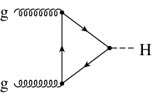
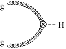
(a)	(b)

Figure 1: Leading order diagram to the process $gg\to H$: (a) in the full and (b) in the effective theory. The “$\otimes$” denotes the effective vertex of Eq. (2).

The leading order result has been known for quite a while [4]. At the parton level it reads:

$$\begin{split}\sigma_{\mbox{\tiny LO}}(gg\to H)&={G_{\mbox{{\tiny F}}}\alpha_{s}^{2}(\mu^{2})\over 128\sqrt{2}\pi}\,\tau^{2}\,\delta(1-z)\,\left|1+(1-\tau)f(\tau)\right|^{2}\,,\\[10.00002pt] f(\tau)&=\left\{\begin{array}[]{ll}\arcsin^{2}{1\over\sqrt{\tau}}\,,&\tau\geq 1\,,\\ -{1\over 4}\left[\log{1+\sqrt{1-\tau}\over 1-\sqrt{1-\tau}}-i\pi\right]^{2}\,,&\tau<1\,,\end{array}\right.\\[10.00002pt] \tau&={4M_{\mathrm{t}}^{2}/M_{\mathrm{H}}^{2}}\,,\qquad z={M_{\mathrm{H}}^{2}/s}\,,\end{split}$$ (1)

where $s$ is the partonic cms energy and $G_{\mbox{{\tiny F}}}$ is the Fermi coupling constant. $\alpha_{s}$ is the strong coupling constant which depends on the renormalization scale $\mu$. $M_{\mathrm{t}}$ is the pole mass of the top quark, and $M_{\mathrm{H}}$ is the Higgs mass. In order to arrive at the cross section for hadron collisions, $\sigma_{\mbox{\tiny LO}}$ has to be folded with the gluon distribution functions.

The currently favored values for the Higgs mass appear to be not too different from the top quark mass. However, since the threshold for open top production is at $M_{\mathrm{H}}=2M_{\mathrm{t}}$, an expansion in terms of small Higgs mass is expected to work well for $M_{\mathrm{H}}<2M_{\mathrm{t}}$. In fact, for the most interesting mass range of 100 GeV $\lesssim M_{\mathrm{H}}\lesssim$ 200 GeV it appears that at next-to-leading order in $\alpha_{s}$ the complete result is excellently approximated by the leading term in an expansion in $M_{\mathrm{H}}^{2}/M_{\mathrm{t}}^{2}$ [5, 6]. Therefore we think it is reasonable to adopt this limit also at next-to-next-to-leading order (NNLO).

All calculations in this paper have been performed using dimensional regularization in $D=4-2\epsilon$ space time dimensions. Unless stated otherwise, renormalized expressions are to be understood in the $\overline{\mbox{\small\sc{MS}}}$ scheme, bare ones will be marked by the superscript “B”. Furthermore, all the quantities used in the following refer to the five flavor effective theory. For example, by $\alpha_{s}$ we mean the running coupling constant with five active flavors, $\alpha_{s}^{(5)}(\mu^{2})$.

The most convenient way to obtain the leading term in $M_{\mathrm{H}}^{2}/M_{\mathrm{t}}^{2}$ is to use the following effective Lagrangian for the Higgs-gluon interaction, where the top quark has been integrated out:

$${\cal L}_{\mathrm{eff}}=-{H\over v}C_{1}^{\mbox{\tiny B}}\,{1\over 4}(G_{\mu\nu}^{\mbox{\tiny B}})^{2}=-{H\over v}C_{1}\,{1\over 4}(G_{\mu\nu})^{2}\,.$$ (2)

Here, $G_{\mu\nu}$ is the gluonic field strength tensor in the effective five flavor theory, and $v$ is the vacuum expectation value of the Higgs field, related to the Fermi constant by $v=(\sqrt{2}G_{\mbox{{\tiny F}}})^{-1/2}$. The coefficient function $C_{1}$ has been computed in [7] up to ${\cal O}(\alpha_{s}^{4})$. In order to obtain the cross section for $gg\to H$ with NNLO accuracy, however, it will only be needed up to ${\cal O}(\alpha_{s}^{3})$ [8]:

$$\begin{split}C_{1}=&-{1\over 3}{\alpha_{s}\over\pi}\bigg{\{}1+{11\over 4}{\alpha_{s}\over\pi}+\left({\alpha_{s}\over\pi}\right)^{2}\bigg{[}{2777\over 288}+{19\over 16}l_{t}+n_{l}\bigg{(}-{67\over 96}+{1\over 3}l_{t}\bigg{)}\bigg{]}\bigg{\}}\,,\end{split}$$ (3)

where $l_{t}=\ln(\mu^{2}/M_{t}^{2})$, with $M_{t}$ the on-shell top quark mass. Here and in the following, the number of (light) flavors $n_{l}$ will eventually be set to five.

The renormalized operator in Eq. (2) is related to the bare one through [9]

$$(G_{\mu\nu})^{2}={1\over 1-\beta({\cal N}\alpha_{s})/\epsilon}(G_{\mu\nu}^{\mbox{\tiny B}})^{2}\,,$$ (4)

where

$${\cal N}=\exp\left[\epsilon\left(-\gamma_{\mbox{\tiny E}}+\ln 4\pi\right)\right]\,,$$ (5)

and $\beta(\alpha_{s})$ governs the running of the strong coupling constant:

$$\mu^{2}{{\rm d}\over{\rm d}\mu^{2}}\alpha_{s}=\alpha_{s}\beta(\alpha_{s})\,.$$ (6)

Its perturbative expansion is known up to ${\cal O}(\alpha_{s}^{4})$ [10], but for the present purpose the terms up to ${\cal O}(\alpha_{s}^{2})$ are sufficient:

$$\begin{split}\beta(\alpha_{s})=&-{\alpha_{s}\over\pi}\bigg{[}{1\over 4}\left(11-{2\over 3}n_{l}\right)+{\alpha_{s}\over\pi}{1\over 16}\left(102-{38\over 3}n_{l}\right)\bigg{]}\,.\end{split}$$ (7)

Using the Lagrangian of Eq. (2) for the Higgs-gluon interaction instead of the full SM, the number of loops reduces by one. For example, in leading order one obtains the tree diagram shown in Fig. 1 (b). The corresponding expression for the partonic cross section is

$$\sigma_{\mbox{\tiny LO}}(gg\to H)={G_{\mbox{{\tiny F}}}M_{\mathrm{H}}^{2}\alpha_{s}^{2}\over 288\sqrt{2}\pi}\,\delta(1-z)$$ (8)

and coincides with the limit $\tau\to\infty$ of Eq. (1), of course.

Going to higher order, one has to compute virtual corrections to diagram Fig. 1 (b). However, these will contain infra-red and collinear divergences. The infra-red divergences will be canceled when adding the corrections from real radiation of quarks and gluons, but the sum will still have collinear divergences. The latter will disappear only when the Altarelli-Parisi splitting functions are taken into account up to the appropriate order [11]. At the next-to-leading order, a full calculation has been carried out in [5]. The correction terms increase the cross section by about a factor of 1.5 to 2 in the relevant Higgs mass range.

At NNLO, only a few ingredients for the full answer are available: In [12] the one-loop amplitude for the radiation of a single quark or gluon in gluon-gluon, gluon-quark, and quark-quark fusion was obtained, and [13] contains the tree-level amplitude for the double-emission of gluons and quarks in these reactions. Both of these results still have to be integrated over the corresponding two- and three-particle phase space, which certainly is a rather non-trivial task by itself.

In this paper, we want to add the virtual two-loop corrections to the list of available knowledge at NNLO. Together with the phase-space integrated expressions for the real radiation and the Altarelli-Parisi splitting functions[11], one will then be able to arrive at a finite result for the partonic cross section. In order to obtain a physically accessible quantity, one needs to fold this partonic result with the corresponding parton distribution functions. However, they have yet to be evaluated to the appropriate order in $\alpha_{s}$ (see, e.g. [14]).

3 Calculation of the two-loop diagrams

Examples of diagrams contributing to the virtual two-loop corrections to the process $gg\to H$ are shown in Fig. 2. The Higgs boson couples to the effective vertex resulting from the Lagrangian of Eq. (2). The two gluons are on-shell ($p_{1}^{2}=p_{2}^{2}=0$), which is why — after extraction of the tensor structure — the diagrams depend only on one kinematic variable, $(p_{1}+p_{2})^{2}=q^{2}=M_{\mathrm{H}}^{2}$.

(a)	(b)	(c)
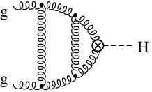
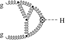
(d)	(e)	(f)

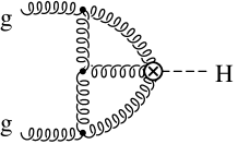
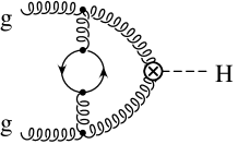
Figure 2: Sample two-loop diagrams contributing to $gg\to H$ at NNLO. The right vertex stands for the effective coupling of the Higgs particle to gluons. The bubble in diagram (e) represents any quark except for the top quark.

In addition to their topology and the power of the denominators, the resulting integrals can be classified by the power of irreducible numerators, i.e. invariants of momenta that cannot be expressed in terms of denominators. In [15, 16], the integrals with unit (or zero) power of denominators and low powers of irreducible numerators were evaluated using Feynman parameterization and dispersion techniques.

In [17] recurrence relations based on the integration-by-parts algorithm [18] for the planar two-loop integrals were derived, reducing them to convolutions of one-loop integrals. These relations allow to compute any such planar diagram with arbitrary powers of the denominators and irreducible numerators.

In our case, however, we also need to compute non-planar diagrams, e.g. Fig. 2 (b). For this reason, we follow an algorithm that has recently been published by Baikov and Smirnov [1]. It relates the recurrence relations for $l$-loop integrals with $n+1$ external legs to the ones for ($l+1$)-loop integrals with $n$ external legs. Here we have $n=l=2$, and thus the massless two-loop vertex diagrams of Fig. 2 are mapped onto massless three-loop two-point functions. The algorithm to compute the latter ones is known [18] and implemented in the computer program MINCER [19], written in FORM [20]. Following the recipe of [1], we modified the MINCER routines such that they are applicable to the class of two-loop three-point functions at hand. For the generation of the diagrams we used QGRAF [21] as integrated in the program package GEFICOM [22].

The only integral that can not be reduced to convolutions of one-loop integrals in this approach is the non-planar one with all propagators appearing in single power, and with numerator equal to one. However, the result for this integral is known as an expansion in $\epsilon$ up to its finite part [15].

As a check of our setup we re-did the calculation of the electro-magnetic quark form factor in QCD to two loops and found full agreement with [16]. We performed this calculation in a general $R_{\xi}$ gauge and explicitly checked its gauge parameter independence in this way. We also computed the two-loop three-gluon vertex in $R_{\xi}$ gauge with two gluons on-shell and found agreement with [17, 23, 24]. Finally, the calculation of the present paper was also performed in $R_{\xi}$ gauge and we verified that the gauge parameter dependence disappears in the sum of all diagrams.

4 Results

The virtual cross section for the process $gg\to H$ can be written as

$$\sigma_{\mathrm{virt}}=4\pi{M_{\mathrm{H}}^{2}\over v^{2}}\,\delta\!\left(1-z\right)\,\left({C_{1}\over 1-\beta({\cal N}\alpha_{s})/\epsilon}\right)^{2}{1\over 256(1-\epsilon)^{2}}\sum_{\rm pol}\left|{\cal M}\right|^{2}\,,$$ (9)

where

$${\cal M}=\varepsilon^{a,\mu}(p_{1},\lambda_{1})\varepsilon^{b,\nu}(p_{2},\lambda_{2}){\cal A}_{\mu\nu}^{ab}(p_{1},p_{2})\,,$$ (10)

and $C_{1}$ is the coefficient function given in Eq. (3). The factor $1/256/(1-\epsilon)^{2}$ comes from the average over initial state polarizations and color. The kinematical constraint on the momenta is

$$p_{1}+p_{2}=q\,,\qquad q^{2}=M_{\mathrm{H}}^{2}\,,\qquad p_{1}^{2}=p_{2}^{2}=0\,.$$ (11)

$\varepsilon^{a,\mu}(p,\lambda)$ is the polarization vector of a gluon with momentum $p$ and polarization $\lambda$, and $a,b$, respectively $\mu,\nu$ are the SU(3)-color and the Lorentz indices. Adopting a covariant $R_{\xi}$ gauge, the polarization vectors obey the relation

$$\sum_{\lambda}\varepsilon^{a\ast}_{\mu}(p,\lambda)\varepsilon^{b}_{\nu}(p,\lambda)=-g_{\mu\nu}\delta^{ab}\,.$$ (12)

The tensor ${\cal A}_{\mu\nu}^{ab}$ may be written as

$${\cal A}_{\mu\nu}^{ab}={\delta^{ab}\over 2M_{\mathrm{H}}^{2}}\left[a\,(p_{1}\cdot p_{2})g_{\mu\nu}+b\,p_{1\nu}p_{2\mu}+c\,p_{1\mu}p_{2\nu}+d\,p_{1\mu}p_{1\nu}+e\,p_{2\mu}p_{2\nu}\right]\,.$$ (13)

The last two terms seem to violate gauge invariance. However, to lowest order they vanish, and starting from next-to-leading order, their contribution to the squared matrix element gets canceled by the diagrams with ghosts in the initial state. We explicitly checked this cancelation by computing these ghost diagrams to the corresponding order. Further, we have

$$a=-b\,,$$ (14)

and thus the $c$ term in (13) does not contribute to the total rate. Therefore we will only quote the result for $a$ in the following. Its loop expansion can be written as

$$a=1+{\alpha_{s}^{\mbox{\tiny B}}\over\pi}\,a^{(1)}+\left({\alpha_{s}^{\mbox{\tiny B}}\over\pi}\right)^{2}a^{(2)}+\ldots\,.$$ (15)

The first order correction has been computed in [5] up to the finite part. Since it involves a second order pole in $\epsilon$ and we are also interested in the finite part of its square, we need its expansion up to $\epsilon^{2}$:

$$\begin{split}a^{(1)}={\cal N}\left(-{\mu^{2}\over M_{\mathrm{H}}^{2}}\right)^{\epsilon}\bigg{\{}-{3\over 2\epsilon^{2}}+{3\over 4}\,\zeta_{2}+\epsilon\,\bigg{(}-{3\over 2}+{7\over 2}\,\zeta_{3}\bigg{)}+\epsilon^{2}\,\bigg{(}-{9\over 2}+{141\over 32}\,\zeta_{4}\bigg{)}\bigg{\}}+{\cal O}(\epsilon^{3})\,,\end{split}$$ (16)

where $\mu$ is the ’t Hooft mass, and $\zeta_{n}\equiv\zeta(n)$ is Riemann’s zeta function ($\zeta_{2}=\pi^{2}/6$; $\zeta_{3}\approx 1.20206$; $\zeta_{4}=\pi^{4}/90$). Furthermore, it is understood that $(-1)^{\epsilon}\equiv\exp(+i\epsilon\pi)$.

To this we add the second order correction:

$$\begin{split}a^{(2)}&={\cal N}^{2}\left(-{\mu^{2}\over M_{\mathrm{H}}^{2}}\right)^{2\epsilon}\bigg{\{}{9\over 8\epsilon^{4}}+{1\over\epsilon^{3}}\,\bigg{[}-{33\over 32}+{1\over 16}\,n_{l}\bigg{]}+{1\over\epsilon^{2}}\,\bigg{[}-{67\over 32}-{9\over 16}\,\zeta_{2}+{5\over 48}\,n_{l}\bigg{]}\\ &+{1\over\epsilon}\,\bigg{[}{17\over 12}+{99\over 32}\,\zeta_{2}-{75\over 16}\,\zeta_{3}+n_{l}\,\bigg{(}-{19\over 72}-{3\over 16}\,\zeta_{2}\bigg{)}\bigg{]}\\ &+{5861\over 288}+{201\over 32}\,\zeta_{2}+{11\over 16}\,\zeta_{3}-{189\over 32}\,\zeta_{4}+n_{l}\,\bigg{[}-{605\over 216}-{5\over 16}\,\zeta_{2}-{7\over 8}\,\zeta_{3}\bigg{]}\bigg{\}}\,,\end{split}$$ (17)

where, as before, $n_{l}$ is the number of light quark flavors, $n_{l}=5$.

Ultra-violet renormalization of the strong coupling constant is given by $\alpha_{s}^{\mbox{\tiny B}}=Z_{\alpha}({\cal N}\alpha_{s})\cdot\alpha_{s}$, where $Z_{\alpha}$ is related to the $\beta$ function of Eq. (7) through

$$\alpha_{s}{\partial\over\partial\alpha_{s}}\ln Z_{\alpha}(\alpha_{s})={\beta(\alpha_{s})\over\epsilon-\beta(\alpha_{s})}\,.$$ (18)

5 Ratio of time-like to space-like form factor

Both as a check and as an estimate on the magnitude of the corrections, we may consider the ratio of the time-like to the space-like form factor. It is free from infra-red singularities and contains the presumably most significant contributions stemming from the analytic continuation of the factor $(\mu^{2}/(-q^{2}))^{\epsilon}$ from space-like to time-like values of $q^{2}$.

As was shown in [25] for the quark form factor in QCD [16], this ratio can be derived up to ${\cal O}(\alpha_{s}^{2})$ from the one-loop terms of the form factor by combining them with a known two-loop anomalous dimension. In the case of $gg\to H$ this anomalous dimension is given by $9/4$ times the one given in [25]. Following the derivation of [25] and setting $\mu^{2}=M_{\mathrm{H}}^{2}$, we arrive at the following expression:

$$\begin{split}\left|{a(M_{\mathrm{H}}^{2})\over a(-M_{\mathrm{H}}^{2})}\right|^{2}&=1+{3\over 2}\,\pi^{2}\,{\alpha_{s}(M_{\mathrm{H}}^{2})\over\pi}+\left({\alpha_{s}(M_{\mathrm{H}}^{2})\over\pi}\right)^{2}\left({3\over 4}\,\pi^{4}+{67\over 8}\,\pi^{2}-{5\over 12}\,\pi^{2}\,n_{l}\right)+{\cal O}(\alpha_{s}^{3})\\ &\approx 1+14.8{\alpha_{s}(M_{\mathrm{H}}^{2})\over\pi}+153.2\left({\alpha_{s}(M_{\mathrm{H}}^{2})\over\pi}\right)^{2}+{\cal O}(\alpha_{s}^{3})\\ &\approx 1+0.528+0.172\approx 1.700\,,\end{split}$$ (19)

where we inserted $n_{l}=5$ in the second line. The third line displays separately the LO, NLO and the NNLO contribution, as well as their sum, for $\alpha_{s}(M_{\mathrm{H}}^{2})=0.112$. Eq. (19) fully agrees with a direct evaluation of the ratio using the expressions (15), (16), and (17) for $a$. This provides a check on the terms $\propto\alpha_{s}^{n}/\epsilon^{2n-k}$ ($k=0,1,2$) of our result. The numerical value of the NLO correction in Eq. (19) reflects the largeness of the full NLO terms as obtained in [5]. The number for the NNLO corrections gives some hope towards a certain degree of convergence for the perturbative series of the full result for $\sigma(gg\to H)$. Concluding this section, let us note that an interesting extension of this discussion could be the resummation of the leading terms along the lines of [26].

6 Conclusions and Outlook

We used the recently introduced method of [1] in order to calculate the NNLO virtual corrections to the production cross section of Higgs bosons in gluon fusion. The result is a gauge invariant component of the full cross section. The next step towards a complete answer for the NNLO rate is to integrate the squared amplitudes for the real radiation processes over the phase space. This is work in progress [27]. Finally, one has to convolute the full partonic cross section with the parton distribution functions. Their evaluation to the relevant order is therefore certainly a very important task.

References

- [1] P.A. Baikov and V.A. Smirnov, Phys. Lett. B 477 (2000) 367.
-
[2]
See
http://lepewwg.web.cern.ch/LEPEWWG/for updates. - [3] M. Spira, A. Djouadi, D. Graudenz, and P.M. Zerwas, Nucl. Phys. B 453 (1995) 17; M. Spira, Fortschr. Phys. 46 (1998) 203.
- [4] F. Wilczek, Phys. Rev. Lett. 39 (1977) 1304; J. Ellis, M. Gaillard, D. Nanopoulos, and C. Sachrajda, Phys. Lett. B 83 (1979) 339; H. Georgi, S. Glashow, M. Machacek, and D. Nanopoulos, Phys. Rev. Lett. 40 (1978) 692; T. Rizzo, Phys. Rev. D 22 (1980) 178.
-
[5]
A. Djouadi, M. Spira, and P.M. Zerwas, Phys. Lett. B 264 (1991) 440;
S. Dawson, Nucl. Phys. B 359 (1991) 283. - [6] S. Dawson and R.P. Kauffman, Phys. Rev. D 49 (1994) 2298.
- [7] K.G. Chetyrkin, B.A. Kniehl, and M. Steinhauser, Nucl. Phys. B 510 (1998) 61.
- [8] K.G. Chetyrkin, B.A. Kniehl, and M. Steinhauser, Phys. Rev. Lett. 79 (1997) 353; M. Krämer, E. Laenen, and M. Spira, Nucl. Phys. B 511 (1998) 523.
- [9] V.P. Spiridonov, Rep. No. INR P-0378 (Moscow, 1984); V.P. Spiridonov and K.G. Chetyrkin , Yad. Fiz. 47 (1988) 818.
- [10] T. van Ritbergen, J.A.M. Vermaseren, and S.A. Larin, Phys. Lett. B 400 (1997) 379.
- [11] G. Curci, W. Furmanski, and R. Petronzio, Nucl. Phys. B 175 (1980) 27.
- [12] C.R. Schmidt, Phys. Lett. B 413 (1997) 391.
- [13] S. Dawson and R.P. Kauffman, Phys. Rev. Lett. 68 (1992) 2273; R.P. Kauffman, S.V. Desai, and D. Risal, Phys. Rev. D 55 (1997) 4005; (E) ibid. D 58 (1998) 119901.
- [14] S. Moch and J.A.M. Vermaseren, proc. Zeuthen Workshop on Elementary Particle Theory: Loops and Legs in Quantum Field Theory, Königstein-Weißig, Germany, 9-14 Apr 2000; hep-ph/0006053.
- [15] R.J. Gonsalves, Phys. Rev. D 28 (1983) 1542.
-
[16]
G. Kramer and B. Lampe,
Z. Phys. C 34 (1987) 497; (E) ibid. 42 (1989) 504;
T. Matsuura, S.C. van der Marck and W.L. van Neerven, Nucl. Phys. B 319 (1989) 570. - [17] A.I. Davydychev and P. Osland, Phys. Rev. D 59 (1998) 014006.
-
[18]
F.V. Tkachov, Phys. Lett. B 100 (1981) 65;
K.G. Chetyrkin and F.V. Tkachov, Nucl. Phys. B 192 (1981) 159. - [19] S.A. Larin, F.V. Tkachov, and J.A.M. Vermaseren, Rep. No. NIKHEF-H/91-18 (Amsterdam, 1991).
- [20] J.A.M. Vermaseren, Symbolic Manipulation with FORM, CAN (1991).
- [21] P. Nogueira, J. Comp. Phys. 105 (1993) 279.
- [22] K.G. Chetyrkin and M. Steinhauser, unpublished.
- [23] A.I. Davydychev, P. Osland, and O.V. Tarasov, Phys. Rev. D 54 (1996) 4087; (E) ibid. 59 (1999) 109901.
- [24] M.A. Nowak, M. Praszałowicz, and W. Słomiński, Ann. Phys. 166 (1986) 443.
- [25] L. Magnea and G. Sterman, Phys. Rev. D 42 (1990) 4222.
- [26] L. Magnea, Rep. No. DFTT 22/00 (Torino, 2000); hep-ph/0006255.
- [27] R.V. Harlander and W.B. Kilgore, in preparation.